Evaluation of Machine Learning Approaches for Hydration Heat Prediction in Energy-Efficient Cement Composites

Abstract

Accurate prediction of the heat of hydration is essential for designing low-emission, durable mortars and concretes with controlled thermal behavior, as the partial replacement of Portland cement clinker with supplementary cementitious materials (SCMs) fundamentally alters hydration kinetics. Although hydration heat can be measured experimentally, such tests are often time-consuming and labor-intensive. Machine learning (ML)-based prediction methods offer a promising alternative, but identifying the most effective model is necessary before practical application. This study evaluates the performance of three ML algorithms, CatBoost, ExtraTrees, and XGBoost, in predicting the heat of hydration in energy-efficient cementitious composites containing SCMs. A dataset of 51 experimental samples was analyzed, comprising mix composition parameters (temperature, slag, fly ash content, and water-to-binder ratio) and four output variables: heat release rate and total heat released after 12, 72, and 168 h. Model performance was assessed using cross-validation and performance metrics (MAE, RMSE, MAPE, R²). All tested models showed a high level of fit (R² > 0.9 for short-term predictions). ExtraTrees demonstrated the most consistent performance, particularly for hydration heat and heat rate estimation, while XGBoost showed superior accuracy for early-age heat evolution. Residual analyses confirmed model stability and minimal bias. The results indicate that ML-based modeling can significantly reduce laboratory workload and enhance understanding of hydration behavior in low-carbon cementitious systems.

1. Introduction

Modern construction faces one of the greatest environmental challenges of the 21st century in the urgent need to reduce carbon dioxide (CO₂) emissions from the cement industry, which accounts for approximately 7–8% of global greenhouse gas emissions [1,2]. Portland cement, the primary binder used in concrete, is the main contributor to these emissions both due to the clinker burning process and the significant energy demand associated with its production. Consequently, one of the key directions of contemporary research is the development of energy-efficient and low-emission cement composites, in which a portion of Portland clinker is replaced by supplementary cementitious materials (SCMs) with a lower carbon footprint, such as fly ash, blast furnace slag, natural pozzolans, or metakaolin. The goal of these efforts is not only to mitigate CO₂ emissions but also to control the release of hydration heat and improve the long-term durability and microstructural stability of cement-based materials.

Substituting Portland clinker with mineral additives fundamentally alters the hydration mechanism of cement, influencing both the course and intensity of heat release [3,4]. Modified systems typically exhibit slower setting and hardening rates, which help reduce the risk of overheating in massive concrete structures but make it more challenging to predict long-term material performance [4,5]. In this context, understanding the relationship between the composition of a cementitious composite and its hydration behaviour, in both chemical and energetic terms, is crucial. Such knowledge enables the rational design of materials that not only emit less CO₂ during production but also feature optimized hydration kinetics, leading to energy savings throughout the entire life cycle of a structure. Therefore, the analysis of the heat of hydration has become a key tool for evaluating the performance of modern, low-emission cementitious materials.

Cement hydration is a complex chemical reaction between cement minerals and water, resulting in the formation of hydration products responsible for setting and hardening. A fundamental aspect of this process is the heat of hydration, the thermal energy released during the chemical reactions that occur as cement transforms from a plastic mixture into a solid matrix [6,7]. Understanding both the magnitude and temporal evolution of this heat is essential for the design, production, and application of cementitious materials. The heat of hydration is directly linked to the kinetics of the hydration process, which comprises several stages: the initial reaction, the dormant or induction period, the acceleration phase, and the deceleration phase. Characteristic heat peaks, such as the prominent one occurring approximately 10 h after mixing with water, are typically associated with the hydration of alite (C₃S) and the formation of primary calcium silicate hydrate (C-S-H) products. The analysis of hydration heat provides valuable insights into the morphology and crystallinity of these products, which in turn strongly influence the microstructure, mechanical strength, and long-term durability of cement-based systems [8].

Experimental studies have shown that the intensity and profile of heat release are influenced by numerous factors, including the water-to-cement (w/c) ratio, the type and amount of SCMs, and the incorporation of nanomaterials [9,10,11,12]. In energy-efficient composites, where part of the clinker is replaced by materials with lower reactivity, the total heat release decreases, resulting in slower early strength development. However, the pozzolanic reactions that occur later in the curing process promote the formation of denser hydration products, thereby enhancing the long-term durability and integrity of the microstructure. Understanding the mechanisms and time-dependent evolution of hydration heat is therefore essential for optimizing cement composite formulations to achieve a balance between low CO₂ emissions, controlled thermal behaviour, and satisfactory mechanical performance.

Four principal methods are commonly used to measure the heat released during cement hydration: solution calorimetry, isothermal conduction calorimetry, adiabatic calorimetry, and semi-adiabatic calorimetry [13,14]. The first two techniques were developed in the 1930s, when excessive temperature rise in massive concrete structures became a recognized issue. In solution calorimetry, both the test sample and a fully hydrated reference sample are dissolved in a mixture of hydrofluoric and nitric acids, and the hydration heat is determined based on the temperature difference between the two. Although this method (ISO 29582-1 [15], EN 196-8 [16], ASTM C186-13 [17]) allows for long-term measurements, it is labour-intensive, time-consuming, and requires strict safety protocols. Isothermal conduction calorimetry (NT Build 505 [18], ASTM C1702-14 [19], EN 196-11 [20]) measures heat flow at a constant temperature with high precision and sensitivity, making it particularly suitable for investigating the early stages of hydration and comparing the effects of different admixtures. However, it is typically limited to small sample sizes and short test durations. Adiabatic calorimetry, on the other hand, records the temperature increase in a sample while maintaining the surroundings at the same temperature, closely replicating real conditions in massive concrete. Despite its advantages, it demands expensive equipment, long testing times, and lacks standardized procedures. Semi-adiabatic calorimetry, standardized by ISO 29582-2 [21], EN 196-9 [22], and NT Build 480 [23], provides a more practical alternative since it employs good thermal insulation and enables testing of both mortars and concretes but requires frequent calibration and correction for heat losses.

While these methods provide essential insights into the hydration process, they remain time-consuming and require high precision and expert handling. This makes them less practical for large-scale data analysis or rapid formulation screening of new, complex cement composites. In this context, machine learning (ML) has emerged as a powerful complementary approach for modelling and predicting hydration behaviour. ML algorithms can learn from experimental data and predict the evolution of hydration heat based on input variables such as cement composition, SCM type and dosage, w/c ratio, and curing conditions. These data-driven models can significantly reduce testing time, minimize laboratory costs, and enhance predictive accuracy. Moreover, integrating ML with experimental calorimetry enables a more comprehensive understanding of the hydration process, facilitating the development of intelligent, energy-efficient cementitious composites that combine reduced CO₂ emissions with controlled heat release and optimized performance.

In summary, the shift toward sustainable construction materials requires a deep understanding of the heat of hydration in energy-efficient cement composites. Accurate prediction and control of hydration heat are not only vital for assessing material behaviour but also for designing eco-efficient, durable cementitious systems that align with the global goal of reducing the carbon footprint of the construction industry. The integration of traditional calorimetric methods with machine learning-based predictive models represents a promising pathway toward the intelligent design of the next generation of low-emission, high-performance cement-based materials.

In recent years, machine learning models such as CatBoost, ExtraTrees, and XGBoost have been applied to predict key mechanical and physical properties of ordinary, high-performance, recycled, and fiber-reinforced concretes [24,25,26]. Exemplary, ExtraTrees has been used to model compressive, tensile, and flexural strength, successfully capturing nonlinear relationships between mix proportions, additives, curing conditions, and resulting performance [27]. Next, XGBoost has shown high accuracy in forecasting compressive strength, tensile strength, density, and porosity; for instance, in high-performance concrete it achieved the best performance among tested models using eight input variables and 60 samples [27]. Further, XGBoost also provided fast and reliable predictions for pervious concrete, reducing the need for time-consuming experiments [28]. In addition, CatBoost has gained popularity due to its strong performance in nonlinear systems and native handling of categorical data, achieving the highest accuracy in predicting compressive and splitting tensile strength and highlighting influential factors such as water-to-binder ratio, cement content, and fiber content [29]. Finally, hybrid CatBoost–XGBoost models have reached state-of-the-art accuracy for uniaxial compressive strength and enabled uncertainty-aware reliability analyses, offering a powerful framework for advanced concrete strength prediction in civil engineering [28].

This article assesses the performance of three machine learning algorithms, CatBoost, ExtraTrees, and XGBoost, in predicting the heat of hydration in energy-efficient cementitious composites containing supplementary cementitious materials (SCMs). The analysis was conducted on a dataset comprising mixture composition parameters, as well as the rate and total heat release over multiple time intervals. The study presents both the methodology for model evaluation and the results of a comparative analysis, highlighting differences in algorithm performance across the analyzed results. The discussion further addresses the practical implications of applying ML techniques in this context, demonstrating their potential to reduce laboratory workload and enhance understanding of hydration processes in low-carbon cementitious systems.

2. Data and Methods

2.1. Data Collection

The dataset used to develop the machine learning model originated from experimental studies on the heat of hydration of cementitious composites [13,30,31]. All hydration heat measurements were performed using a TAMAir isothermal calorimeter (TA Instruments, New Castle, DE, USA) under controlled laboratory conditions. The analysed dataset comprised 51 measurement records, varying in terms of binder composition, curing temperature, and water-to-binder ratio (w/b). The input variables used for model training included: Ordinary Portland cement content (OPC, %), blast furnace slag content (%), fly ash content (%), water-to-binder ratio (w/b), and curing temperature (°C). The output variables, representing the predicted values, described the hydration process through the cumulative heat of hydration released (J·g⁻¹) after 12, 72, and 168 h, and the maximum heat release rate (J·g⁻¹·h⁻¹). The dataset encompassed both pure Portland cement composites and mixtures incorporating mineral additives (blast furnace slag and fly ash) in various proportions. The diversity in mixture composition, curing temperature, and w/b ratio ensured that the data captured a broad range of hydration behaviours, thus providing a robust foundation for modelling and predicting the thermal evolution of cementitious materials. The dataset was divided into a training set of 45 records (

Table 1. Training set.

No.	OPC	Slag, %	Fly ash, %	w/b	Temperature, °C	Heat Evolved, J·g−1			The Peak Value of Heat Evolution Rate, J·g−1h−1
						After 12 h	After 72 h	After 168 h
1	100	0	0	0.45	30	123.7	303	338.4	14.30
2	100	0	0	0.45	40	161.2	308.3	345.1	20.90
3	40	60	0	0.45	20	34.3	120.8	158.1	3.40
4	40	60	0	0.45	40	69.3	167.4	202.4	8.10
5	40	0	60	0.54	20	23.5	114	144.8	2.90
6	40	0	60	0.54	30	46.4	129.3	156.6	5.10
7	40	30	30	0.49	20	28.9	115	149.5	3.10
8	40	30	30	0.49	30	48.1	133.1	167.4	5.20
9	40	30	30	0.49	40	65.6	159	188.5	7.60
10	100	0	0	0.3	20	73.8	257	320.8	8.20
11	100	0	0	0.3	35	132.1	250.9	250.2	16.10
12	100	0	0	0.3	50	191.3	270.4	258	32.10
13	100	0	0	0.35	20	67.5	252.4	291.6	8.30
14	100	0	0	0.35	35	136.5	275.3	282.4	16.90
15	100	0	0	0.4	20	73.9	251.3	295.4	8.30
16	100	0	0	0.4	35	137.6	282.1	282.3	17.10
17	100	0	0	0.4	50	209.6	291.2	257.7	33.50
18	100	0	0	0.45	20	76.1	254.3	317.8	8.30
19	100	0	0	0.45	35	148.5	311.4	338.6	17.20
20	100	0	0	0.45	50	209.5	272.8	199.8	33.90
21	100	0	0	0.5	20	74.8	249.7	311.5	8.10
22	100	0	0	0.5	35	133.9	294	306.9	15.70
23	100	0	0	0.5	50	218.7	304.7	271.1	35.20
24	100	0	0	0.55	20	78	255.4	319.3	8.30
25	100	0	0	0.55	35	146.6	302.1	315.1	17.50
26	100	0	0	0.55	50	208.4	297	278.7	32.10
27	100	0	0	0.6	20	75.7	251.2	313.5	8.10
28	100	0	0	0.6	35	149.7	311.2	342.6	17.10
29	100	0	0	0.6	50	219.2	290.4	233.4	34.60
30	100	0	0	0.5	20	76.6	269.1	320.1	9.30
31	100	0	0	0.5	50	247.3	319.3	348.2	42.50
32	90	0	10	0.5	20	54.2	218.2	285.3	6.70
33	90	0	10	0.5	50	183.2	266.2	301.2	28.60
34	70	0	30	0.5	50	168.6	248.3	276.5	31.30
35	50	0	50	0.5	20	25.1	141.9	188.6	4.30
36	50	0	50	0.5	50	102.4	172.6	211.2	16.20
37	30	0	70	0.5	20	11.6	93.8	133.4	2.70
38	30	0	70	0.5	50	57.1	94.5	148.6	8.30
39	90	10	0	0.5	20	63.6	236.2	302.3	7.90
40	90	10	0	0.5	50	217.8	309.6	323.2	39.70
41	70	30	0	0.5	20	46.9	186.2	257.3	6.30
42	70	30	0	0.5	50	162.3	249.9	283.3	27.20
43	50	50	0	0.5	20	37.9	154.5	192.1	5.40
44	30	70	0	0.5	20	26.3	112.1	162.7	3.60
45	30	70	0	0.5	50	94.4	170.5	215.2	13.80

) used to fit the model, and a testing set of 6 records (

Table 2. Testing set.

No.	OPC	Slag, %	Fly Ash, %	w/b	Temperature, °C	Heat Evolved, J·g−1			The Peak Value of Heat Evolution Rate, J·g−1h−1
						After 12 h	After 72 h	After 168 h
1	100	0	0	0.45	20	70.1	250.5	315	7.70
2	40	60	0	0.45	30	59.8	151.5	198.2	6.00
3	40	0	60	0.54	40	60.6	148	179.1	7.90
4	100	0	0	0.35	50	218.4	299.9	279.1	33.90
5	70	0	30	0.5	20	41.7	185.7	256.7	5.80
6	50	50	0	0.5	50	129.7	213.5	265.2	18.90

) employed to evaluate its predictive performance.

2.2. Statistical Descriptions and Data Characteristics

The study conducted an exploratory analysis of all numerical variables, including an examination of their distributions and an assessment of relationships between input characteristics and output parameters. Basic descriptive statistics (count, mean, standard deviation, minimum, first quartile, median, third quartile, maximum, and number of missing values) were calculated for both input and output variables (

Table 3. Descriptive statistics of numerical variables.

Variable	Mean	Std	Min	25%	50%	75%	Max
Temperature	33.824	12.8290	20.00	20.00	35.00	50.0	50.00
Slag	11.569	21.6680	0.00	0.00	0.00	10.0	70.00
Fly ash	11.569	21.6680	0.00	0.00	0.00	10.00	70.00
w/b	0.475	0.0710	0.30	0.45	0.50	0.50	0.60
Rate of heat evolution	15.318	11.4390	2.70	7.15	8.30	19.90	42.50
Heat evolved (12 h)	108.196	65.9750	11.60	58.45	76.60	155.45	247.30
Heat evolved (72 h)	226.798	69.5620	93.80	163.20	250.90	286.25	319.30
Heat evolved (168 h)	256.471	64.0170	133.40	199.00	276.50	312.50	348.20

). The dataset contained a total of 51 records, with no missing values identified. The results indicate that most input and output variables exhibit skewed distributions, as evidenced by substantial differences between the mean and median. The accumulation of observations at the minimum value (so-called fixation) suggests that a considerable portion of samples lack a given component, leading to asymmetry in the variable distribution and warranting further consideration. Temperature and output parameters display variable ranges, effectively reflecting the experimental conditions and highlighting the potential for modeling.

The next step involved analyzing the Pearson correlations between variables (Figure 1). The results are presented as a heat map illustrating the relationships among the features. Temperature shows a strong positive correlation with all output parameters-most notably with the rate of heat evolution (r = 0.82) and heat evolved (12 h) (r = 0.79). This suggests that higher temperatures promote hydration and accelerate heat release. In contrast, fly ash and slag display moderate negative correlations with the thermal parameters, indicating that higher proportions of these additives tend to delay or reduce the overall thermal effect. The water-to-binder ratio (w/b) shows weak associations with the output variables within the studied range, generally exhibiting an inverse relationship with the amount of heat released. Additionally, Figure 1 shows very strong correlations among the output variables, with coefficients even reaching up to r ≈ 0.98. Such a high degree of association can be expected in this specific case, as the heat-related outputs originate from the same hydration process. In detail, the rate of heat evolution is closely linked to the cumulative heat measured at 12 h due to the close relation between these response variables (the maximum value of which occurs in the first hours and is a derivative of the released heat). Importantly, this collinearity arises mainly among the output parameters themselves, rather than between the input features and the outputs, indicating that the observed relationships stem from the underlying process of cement hydration rather than from redundancy or information leakage within the predictor set.

The analysis, presented as a scatterplot matrix with superimposed LOWESS curves (Figure 2), complements the statistical analysis. This visualization clearly confirms that the examined input features exert a distinct, though not always simple or linear, influence on the parameters of the hydration process.

2.3. Methods

The first step (Figure 3, Step 1) involved collecting all the necessary experimental and technological data for the tested samples.

Next, the collected data were loaded into a DataFrame structure (Figure 3, Step 2), where they were verified for accuracy and completeness, ensuring that all required columns were present. The data were then converted into numerical format for subsequent analysis.

Given the limited size of the training dataset, the Leave-One-Out Cross-Validation (LOOCV) method (Figure 3, Step 3) was selected to ensure reliable model evaluation. LOOCV is a variant of k-fold cross-validation in which the number of folds equals the number of samples in the dataset. In this approach, each observation is used once as a test instance, while the remaining observations form the training set. The method provides an almost unbiased estimate of prediction error; however, for very small datasets, it can result in high variance of the error estimate [32,33].

Subsequently, the input variables listed in

Table 4. List of Input variables (Features) used in the study.

Variable	Description
Temperature (°C)	Experimental temperature during heat evolution measurement
Slag (%)	Content of ground granulated blast-furnace slag in the binder
Fly ash (%)	Content of fly ash in the binder
w/b ratio	Water-to-binder ratio (mass of water divided by total binder content)

and the target variables listed in

Table 5. List of Output variables (Targets) used in the Study.

Variable	Description
Rate of heat evolution (J·g−1h−1)	Peak rate of heat release during hydration (maximum heat flow)
Heat evolved (12 h) (J/g)	Total heat evolved after 12 h of hydration
Heat evolved (72 h) (J/g)	Total heat evolved after 72 h of hydration
Heat evolved (168 h) (J/g)	Total heat evolved after 168 h of hydration

were selected, and the data were divided into training and test sets (Figure 3, Step 4). The training set comprised 45 records, while the test set contained 6 records. The test samples were deliberately chosen to be diverse, ensuring a cross-sectional evaluation of the model across various cases.

The next step (Figure 3, Step 5) involved training three regression models: ExtraTrees, CatBoost, and XGBoost. All three models were tuned before the final evaluation. The tuning procedure combined a systematic GridSearchCV exploration with additional manual refinement to stabilize performance. For the ExtraTrees Regressor, we tested parameter ranges recommended for tree-ensemble models, varying the number of estimators, tree depth, feature subsampling, and minimum leaf sizes. Based on the grid-search results and subsequent adjustments, the final configuration was: n_estimators = 800, max_depth = None, max_features = 0.75, min_samples_split = 2, and min_samples_leaf = 1. For XGBoost, tuning focused on the hyperparameters most influential for gradient-boosting performance, including tree depth, learning rate, subsampling ratios, and the number of boosting rounds. GridSearchCV was used to identify promising parameter regions, after which intermediate values and extended boosting iterations were applied for greater stability. The final configuration was: n_estimators = 2000, learning_rate = 0.03, max_depth = 4, subsample = 0.85, colsample_bytree = 0.85, reg_alpha = 0.5, reg_lambda = 1.0, and min_child_weight = 2. The CatBoost model was tuned using a hybrid approach. An initial grid search over typical hyperparameter ranges (tree depth, learning rate, and L2 regularization) was followed by manual refinement to improve generalization. The final configuration for the multi-target setting was: iterations = 1500, learning_rate = 0.03, depth = 6, l2_leaf_reg = 3.0, with the loss function set to MultiRMSE.

The ExtraTrees (Extremely Randomized Trees) algorithm relies on randomly partitioning the data and constructing multiple decision trees, which increases the diversity of the models within the ensemble. In practice, this method exhibits strong resistance to overfitting and offers good interpretability [34,35]. The CatBoost (Categorical Boosting) model employs gradient boosting over symmetric trees. It automatically encodes categorical variables, eliminating the need for manual preprocessing of input data. Previous studies have demonstrated that this approach provides high stability and accuracy in regression tasks, even when applied to small and heterogeneous datasets [36,37]. The XGBoost (Extreme Gradient Boosting) algorithm is another gradient boosting technique for decision trees that incorporates regularization mechanisms to mitigate overfitting. Literature highlights its high scalability and efficiency in handling large and complex datasets, where the regularization and optimization of sequential decision trees enable superior performance compared to traditional Random Forest models [38,39].

Prediction quality was assessed using Out-of-Fold (OOF) validation based on the Leave-One-Out Cross-Validation (LOOCV) procedure (Figure 3, Step 6). OOF validation for each model on the training set involved calculating performance metrics separately for each target variable. The OOF approach stores predictions for each sample only from models that have not encountered it during training, thereby preventing data leakage. This provides a realistic assessment of the model’s generalization capability and is also useful for computing residuals and aggregating predictions in complex ensemble architectures [40,41].

In this study, the models were evaluated using the following metrics: Mean Absolute Error (MAE) (Equation (1)), Mean Squared Error (MSE) (Equation (2)), Mean Absolute Percentage Error (MAPE) (Equation (3)), and the coefficient of determination (R²) (Equation (4)).

$$\mathrm{M}\mathrm{A}\mathrm{E}: {\displaystyle \frac{1}{n}}\sum _{i=1}^n\left|y_i-\widehat{y_i}\right|$$

(1)

$$\mathrm{M}\mathrm{S}\mathrm{E}: {\displaystyle \frac{1}{n}}\sum _{i=1}^n{\left(y_i-\widehat{y_i}\right)}^2$$

(2)

$$\mathrm{M}\mathrm{A}\mathrm{P}\mathrm{E}: {\displaystyle \frac{100\%}{n}}\sum _{i=1}^n\left|{\displaystyle \frac{y_i-\widehat{y_i}}{y_i}}\right|$$

(3)

$${\mathrm{R}}^2:1-{\displaystyle \frac{{\sum }_{i=1}^n{\left(y_i-\widehat{y_i}\right)}^2}{{\sum }_{i=1}^n{\left(y_i-\overline{y}\right)}^2}}$$

(4)

where:

$y_i$—actual observed values;

$\widehat{y_i}$—predicted values;

$\overline{y}$—mean of actual values;

$n$—number of observations.

Next, the models were trained on the complete training set, and predictions were generated for an independent external test set (Figure 3, Step 7). The results were subsequently presented using the selected performance indicators: Mean Absolute Error (MAE) (Equation (1)), Mean Squared Error (MSE) (Equation (2)), Mean Absolute Percentage Error (MAPE) (Equation (3)), and the coefficient of determination (R²) (Equation (4)).

The final stage of the experiment involved presenting the modeling results in both tabular and graphical form (Figure 3, Step 8). Detailed diagnostic analyses were conducted, including an assessment of the distribution and structure of residuals (True vs. Predicted plots, Residuals vs. Predicted plots, residual histograms, and Q-Q plots), as well as statistical tests (Shapiro–Wilk, D’Agostino, and Student’s t-test) to verify the normality, unbiasedness, and stability of the prediction errors.

3. Results

3.1. Model Performance Evaluation

To evaluate the predictive performance of the machine learning models, four complementary statistical metrics were applied: mean absolute error (MAE), root mean square error (RMSE), mean absolute percentage error (MAPE), and the coefficient of determination (R²). Together, these metrics quantify the magnitude of prediction errors and provide a comprehensive assessment of the models’ accuracy.

Table 6. Model performance using MAE per target and model (OOF TRAIN).

	Model	CatBoost	ExtraTrees	XGBoost
Target
Heat evolved (12 h)		12.482	12.090	14.299
Heat evolved (72 h)		18.765	16.350	15.313
Heat evolved (168 h)		27.401	24.109	27.234
Rate of heat evolution		2.595	2.328	2.801

presents the MAE values. Among the tested algorithms, ExtraTrees achieved the lowest MAE in most cases, indicating the highest predictive accuracy. For heat evolved (12–168 h), its errors ranged from 12.090 to 24.109, outperforming both CatBoost and XGBoost, which exhibited larger deviations-particularly after 168 h. The only exception was for heat evolved (72 h), where XGBoost performed slightly better. Similarly, for the rate of heat evolution, ExtraTrees (MAE = 2.328) outperformed CatBoost (MAE = 2.595) and XGBoost (MAE = 2.801).

The RMSE results (

Table 7. Model performance using RMSE per target and model (OOF TRAIN).

	Model	CatBoost	ExtraTrees	XGBoost
Target
Heat evolved (12 h)		16.719	15.774	20.223
Heat evolved (72 h)		25.409	20.969	20.739
Heat evolved (168 h)		35.576	31.590	37.707
Rate of heat evolution		3.738	3.489	4.476

) confirm the trends observed for the MAE. The ExtraTrees model achieved the lowest errors for most target variables-particularly at 12 h, 168 h, and for the Rate of heat evolution-demonstrating its strong overall predictive accuracy. The only exception occurred at 72 h, where XGBoost slightly outperformed ExtraTrees (RMSE = 20.739 vs. 20.969). Nevertheless, the consistently lower RMSE values of ExtraTrees across the remaining targets highlight its robustness in predicting both cumulative and rate-based heat evolution.

A comparison of the models based on MAPE values (

Table 8. Model performance using MAPE per target and model (OOF TRAIN).

	Model	CatBoost	ExtraTrees	XGBoost
Target
Heat evolved (12 h)		0.199	0.182	0.178
Heat evolved (72 h)		0.112	0.092	0.076
Heat evolved (168 h)		0.120	0.103	0.110
Rate of heat evolution		0.239	0.209	0.245

) indicates that XGBoost performed best overall. For heat evolved after 12 and 72 h, XGBoost achieved the lowest MAPE values (0.178 and 0.076, respectively), demonstrating superior capability in modeling early-stage hydration behavior. After 168 h, however, the ExtraTrees model slightly outperformed the others (0.103 versus 0.110 for XGBoost and 0.120 for CatBoost), suggesting that its ensemble averaging approach may better capture long-term cumulative heat trends. For the rate of heat evolution, ExtraTrees again achieved the lowest MAPE (0.209), followed by CatBoost (0.239) and XGBoost (0.245).

The coefficient of determination (R²) values (

Table 9. Model performance using R² per target and model (OOF TRAIN).

	Model	CatBoost	ExtraTrees	XGBoost
Target
Heat evolved (12 h)		0.935	0.942	0.905
Heat evolved (72 h)		0.869	0.911	0.913
Heat evolved (168 h)		0.703	0.765	0.666
Rate of heat evolution		0.893	0.907	0.847

) confirm that all three models achieved a high degree of fit, particularly during the early stages of hydration. The ExtraTrees model attained the highest R² values at 12 h (0.942) and 168 h (0.765), as well as for the rate of heat evolution (0.907). It was only slightly outperformed by XGBoost (0.913) for heat evolved (72 h), where it achieved an R² of 0.911.

Overall, the comparative analysis of MAE, RMSE, MAPE, and R² demonstrates that the ExtraTrees model provided the most consistent and accurate predictions across the evaluated targets. The XGBoost algorithm also showed strong performance in several cases, while CatBoost generally exhibited lower accuracy, though it occasionally surpassed XGBoost in specific instances. These findings indicate that ExtraTrees offers the best overall balance of precision, robustness, and generalizability among the tested models.

3.2. Residual Analysis of the Machine Learning Models

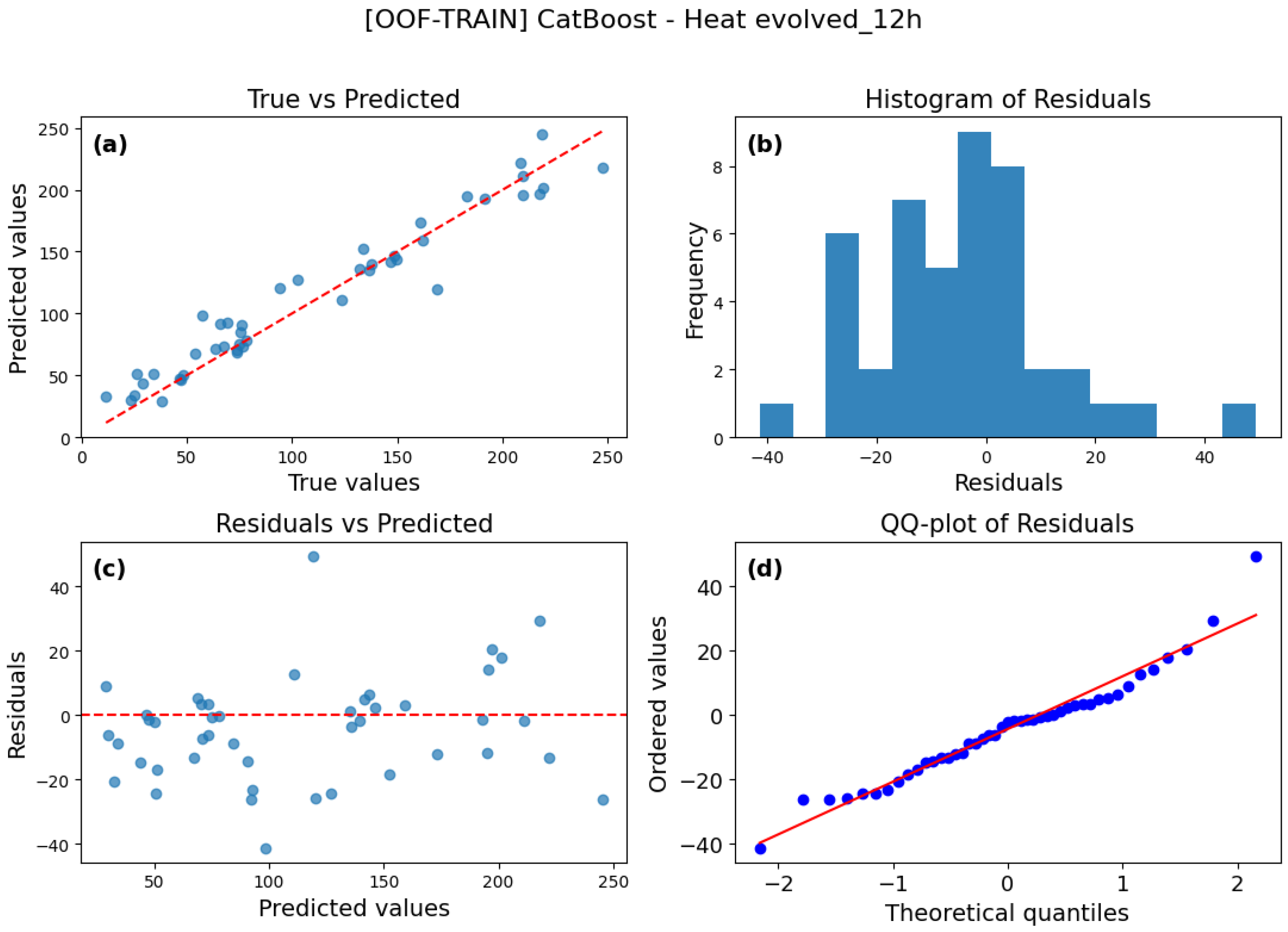
To complement the model evaluation based on error metrics, a residual analysis was conducted for all tested models. This approach enables a more detailed examination of model behavior by assessing the distribution, magnitude, and potential structure of residuals. The analysis includes graphical diagnostics such as True vs. Predicted, Residuals vs. Predicted, histogram of Residuals, and Q-Q plots. These visualizations provide additional insights into model stability, error patterns, and potential dependencies that may influence prediction quality.

In the True vs. Predicted plot (Figure 4a), a clear linear relationship is observed between the actual and predicted values, with most points distributed close to the reference line. Some deviations occur, particularly at higher value ranges, suggesting increased dispersion for larger true values. The histogram of Residuals (Figure 4b) shows an asymmetric distribution, with negative errors prevailing over positive ones. Although the histogram peaks near zero, several positive and negative outliers are present. The Residuals vs. Predicted plot (Figure 4c) indicates that residuals remain generally clustered around zero across the prediction range. They are distributed both above and below the zero line without a distinct directional trend, though a slight increase in dispersion is noticeable for higher predicted values. Finally, the Q-Q plot of residuals (Figure 4d) shows that most points align well with the reference line, suggesting partial conformity to a normal distribution. However, deviations at the extremes indicate the presence of outliers.

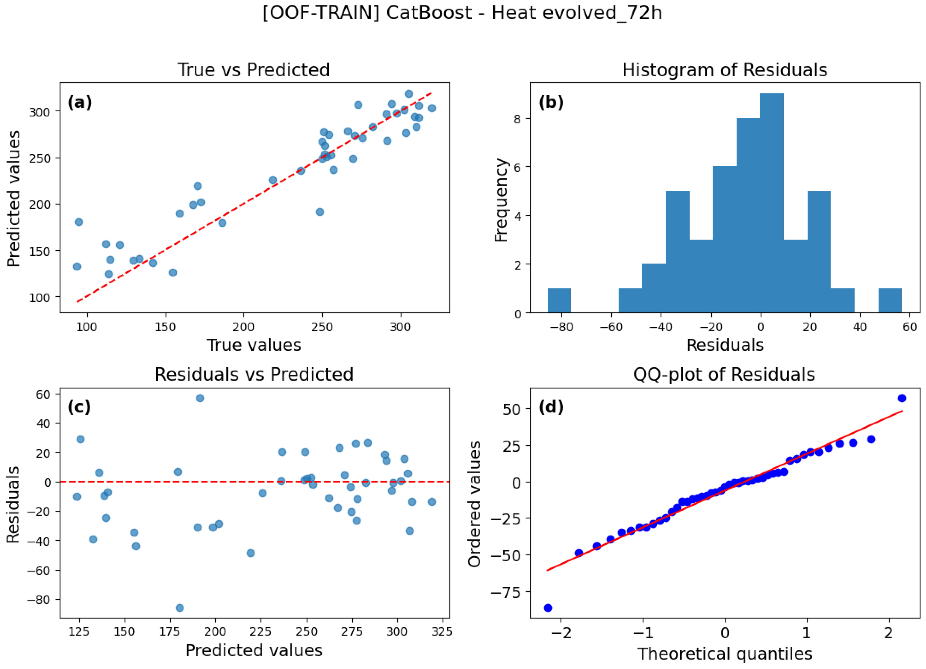
The True vs. Predicted plot (Figure 5a) illustrates the relationship between the actual and predicted values of the CatBoost model for the heat evolved parameter after 72 h. Most points lie along the reference line, indicating good agreement between predictions and observations. However, some dispersion is evident at lower actual values, suggesting greater model deviation in this range. True–Predicted plots are used to assess how closely model estimates follow the ideal 1:1 relationship between observed and predicted values, providing a visual indication of overall model agreement [42]. The histogram of Residuals (Figure 5b) shows a distribution close to normal, with a slight predominance of negative residuals and a few extreme values on both sides. Histograms of residuals are widely applied to evaluate the symmetry and approximate normality of prediction errors, helping to identify skewness or extreme deviations [43]. The Residuals vs. Predicted plot (Figure 5c) indicates that the residuals fluctuate around zero across the prediction range, with a minor increase in dispersion at lower predicted values. Residuals–Predicted plots allow visual inspection of potential bias or heteroscedasticity, as systematic patterns in the residuals may indicate model misspecification [44]. In the Q-Q plot (Figure 5d), the residuals largely follow the reference line, particularly in the central region. Deviations at the distribution tails suggest slight asymmetry or the presence of outliers. Q-Q plots are used to compare the empirical distribution of residuals with the theoretical normal distribution, where alignment with the reference line suggests approximate normality [45].

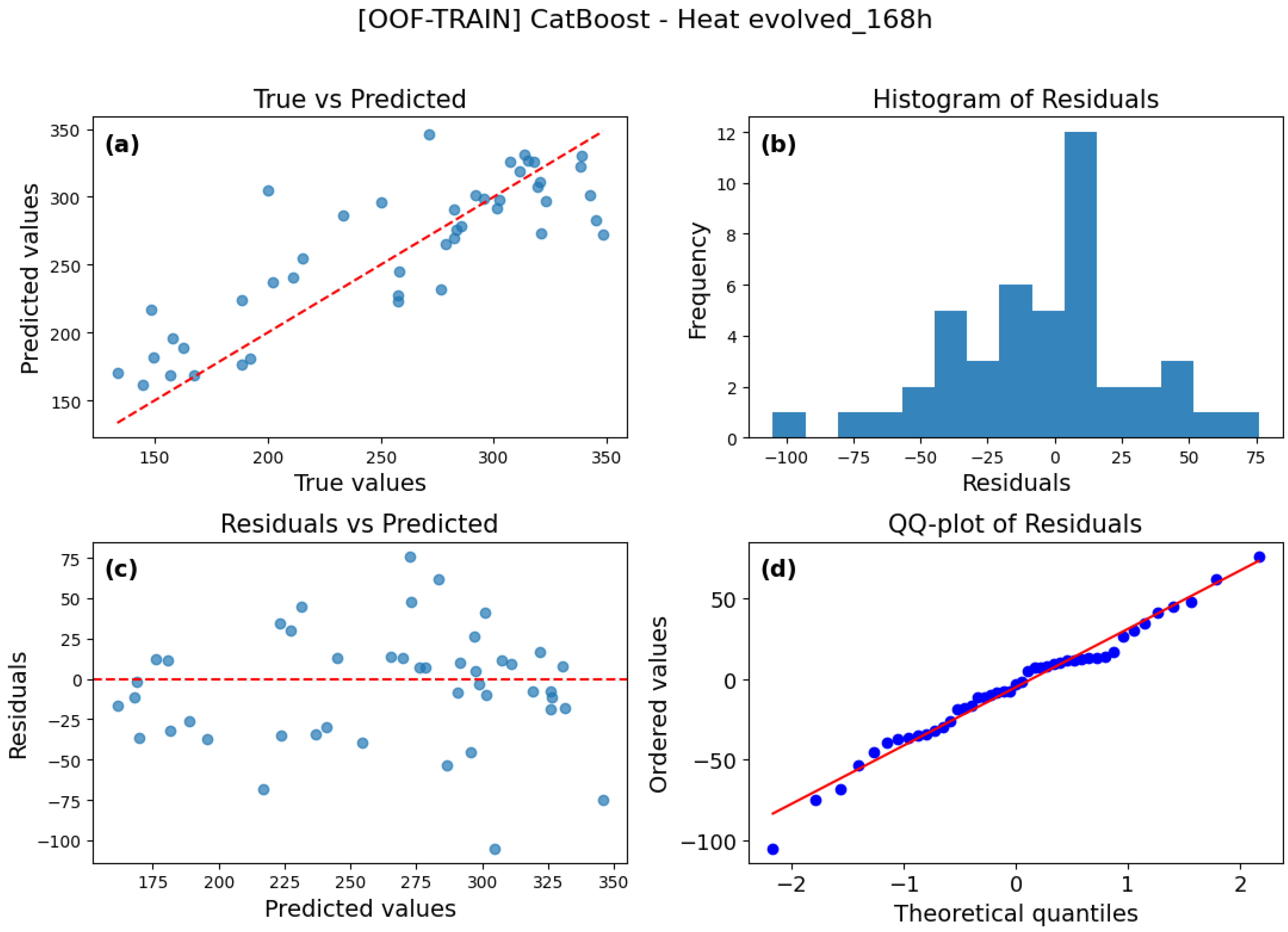
The True vs. Predicted plot (Figure 6a) illustrates the distribution of predicted versus actual values for the CatBoost model and the heat evolved (168 h) variable. Most points lie close to the y = x line, indicating good overall agreement, although moderate scatter is observed both above and below the line across the full value range. In the lower range, predictions tend to be slightly underestimated, while at higher values, both underestimations and overestimations occur. The histogram of Residuals (Figure 6b) shows that most predictions cluster around values slightly above zero, with a distinct peak in the 0–25 range. The distribution is slightly asymmetric, with a minor skew toward negative residuals. The Residuals vs. Predicted plot (Figure 6c) does not reveal any clear systematic trend, though a moderate increase in scatter is noticeable for higher predicted values (above 250), where residuals exhibit larger positive and negative amplitudes. The Q-Q plot (Figure 6d) indicates a general conformity of the residual distribution to normality in the central region, where points align closely with the theoretical reference line. Minor deviations appear at the distribution tails, particularly in the lower part, where several residuals are more negative than expected under a normal distribution.

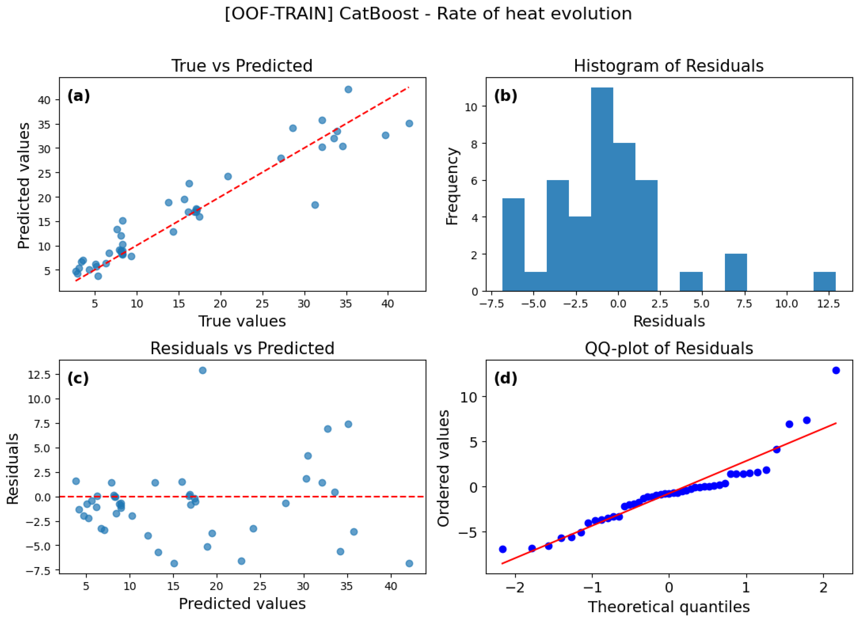
The True vs. Predicted plot (Figure 7a) shows a clear linear relationship between the actual and predicted values for the rate of heat evolution. Most points lie close to the y = x line, indicating strong agreement between predictions and observed data. However, for higher values (above 30), several points fall slightly below the line, suggesting a minor tendency toward underestimation in this range. The histogram of residuals (Figure 7b) peaks between −2.5 and 0, with most cases clustered around slightly negative and near-zero values. Although the highest concentration of residuals appears between −2.5 and 0, a noticeable number of cases also falls within the range of 0 to 2.5. This distribution indicates that the model produces both small underpredictions and small overpredictions, with most errors remaining close to zero on either side. This pattern suggests the absence of a strong directional bias, as the residuals are primarily shaped by natural variability in the data. The Residuals vs. Predicted plot (Figure 7c) shows that residuals are generally distributed around zero across the full prediction range. In the lower prediction range (below approximately 20 units), a predominance of negative residuals is observed, indicating a slight overestimation tendency in this region. At higher values, the scatter increases but remains largely random, without a clear directional pattern. The Q-Q plot (Figure 7d) indicates that the residual distribution aligns well with the normal distribution in the central region. Minor deviations are visible at both tails, particularly in the upper range, where several observations exceed the theoretical values predicted by the normal distribution.

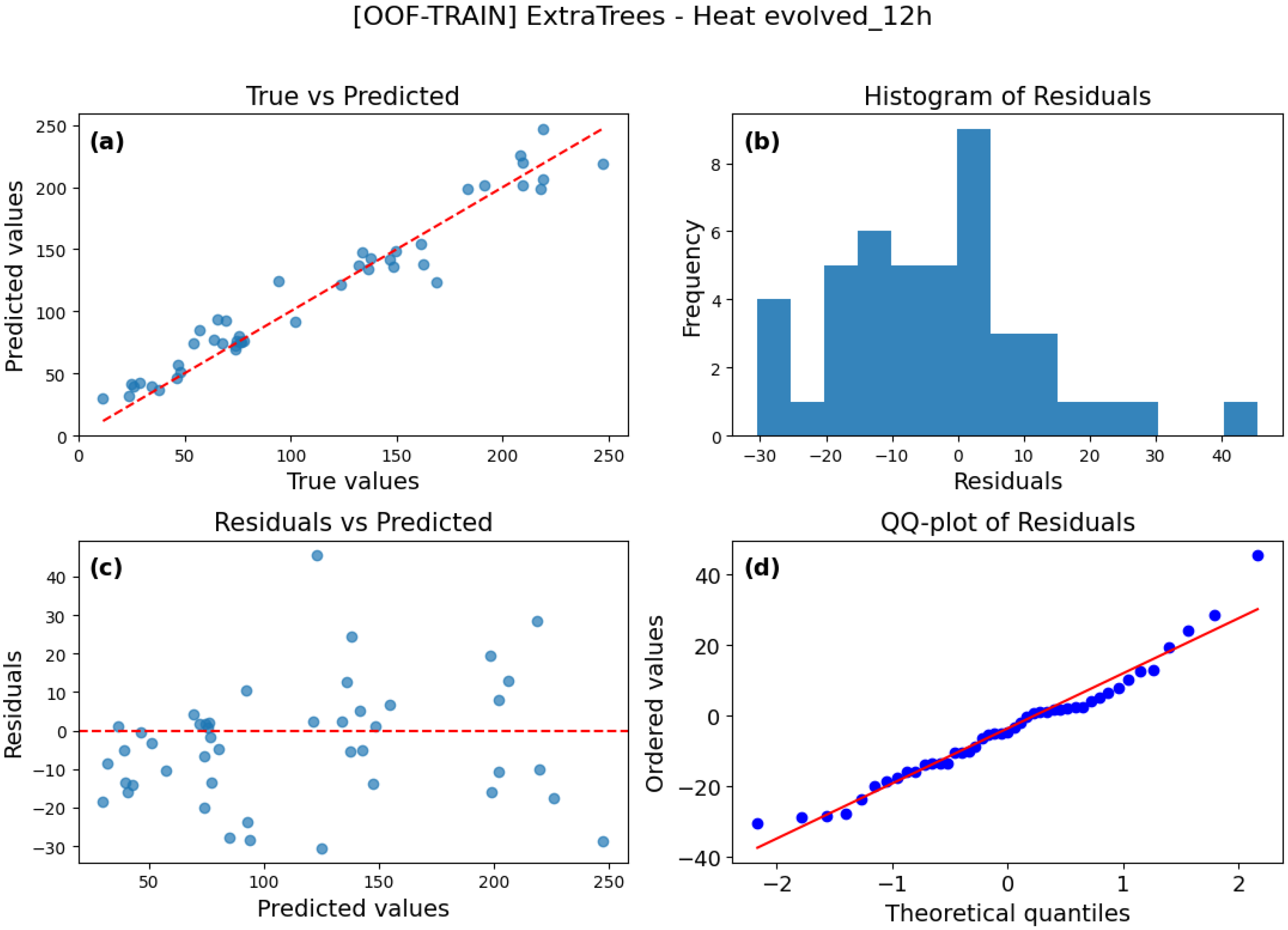
The True vs. Predicted plot (Figure 8a) presents the results of the ExtraTrees model for heat evolved after 12 h. The points are broadly distributed around the y = x line, showing particularly good agreement in the mid-range values, while slightly greater dispersion is observed at higher values. The histogram of Residuals (Figure 8b) reveals an asymmetric error distribution, with a noticeably higher number of negative residuals, suggesting that the model tends to slightly overestimate the predicted values in some cases. Despite this asymmetry, most residuals fall within a relatively narrow range. In the Residuals vs. Predicted plot (Figure 8c), residuals are scattered on both sides of the zero baseline, indicating that the model does not display any significant systematic bias across the prediction range. In the lower prediction range (below 80), a slight predominance of negative residuals can be observed, again suggesting a minor tendency to overestimate in this area. The Q-Q plot (Figure 8d) shows that most points align closely with the reference line in the central part of the distribution, indicating partial conformity to normality. Deviations occur primarily at the tails, especially in the upper part, where several observations exhibit higher-than-expected values.

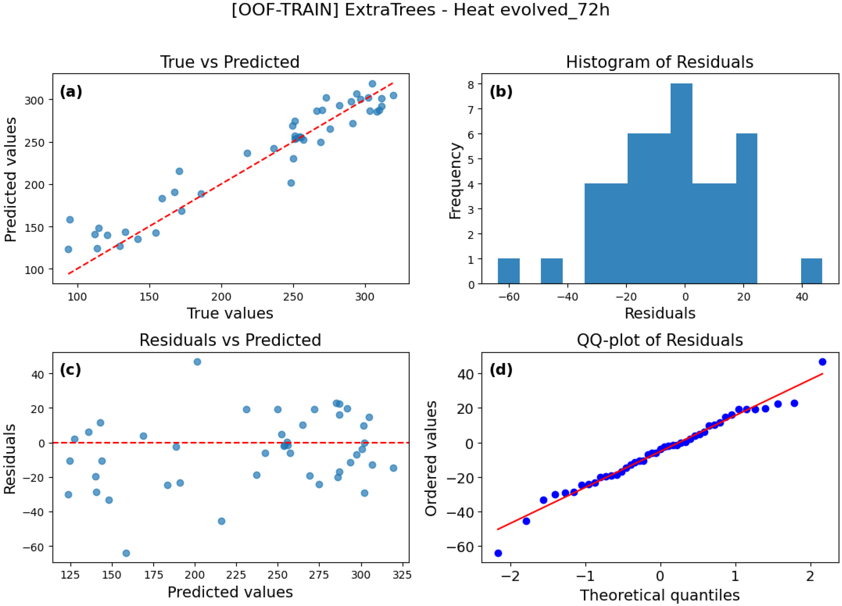
In the True vs. Predicted plot (Figure 9a) for the ExtraTrees model, most points lie close to the perfect-fit (y = x) line, indicating strong agreement between predictions and observations. The scatter around the line appears relatively uniform across the data range, though a few larger deviations are visible at lower values, where some observations are slightly overestimated. High true values are well captured, showing no clear pattern of systematic error. The histogram of Residuals (Figure 9b) displays a relatively symmetrical distribution centered near zero, with most residuals falling within the range of approximately −30 to +20, and only a few distant values. In the Residuals vs. Predicted plot (Figure 9c), points are distributed on both sides of the zero axis, indicating no apparent relationship between error magnitude and predicted value. In the lower prediction range, greater scatter and several more negative residuals appear, suggesting occasional overestimation and one case of significant underestimation. For higher predicted values, errors are smaller and more symmetrically distributed around zero. The Q-Q plot (Figure 9d) shows that points in the central region align closely with the reference line, while larger deviations occur at the distribution tails. These deviations reflect individual outliers but do not significantly affect the overall conformity of residuals to a normal distribution.

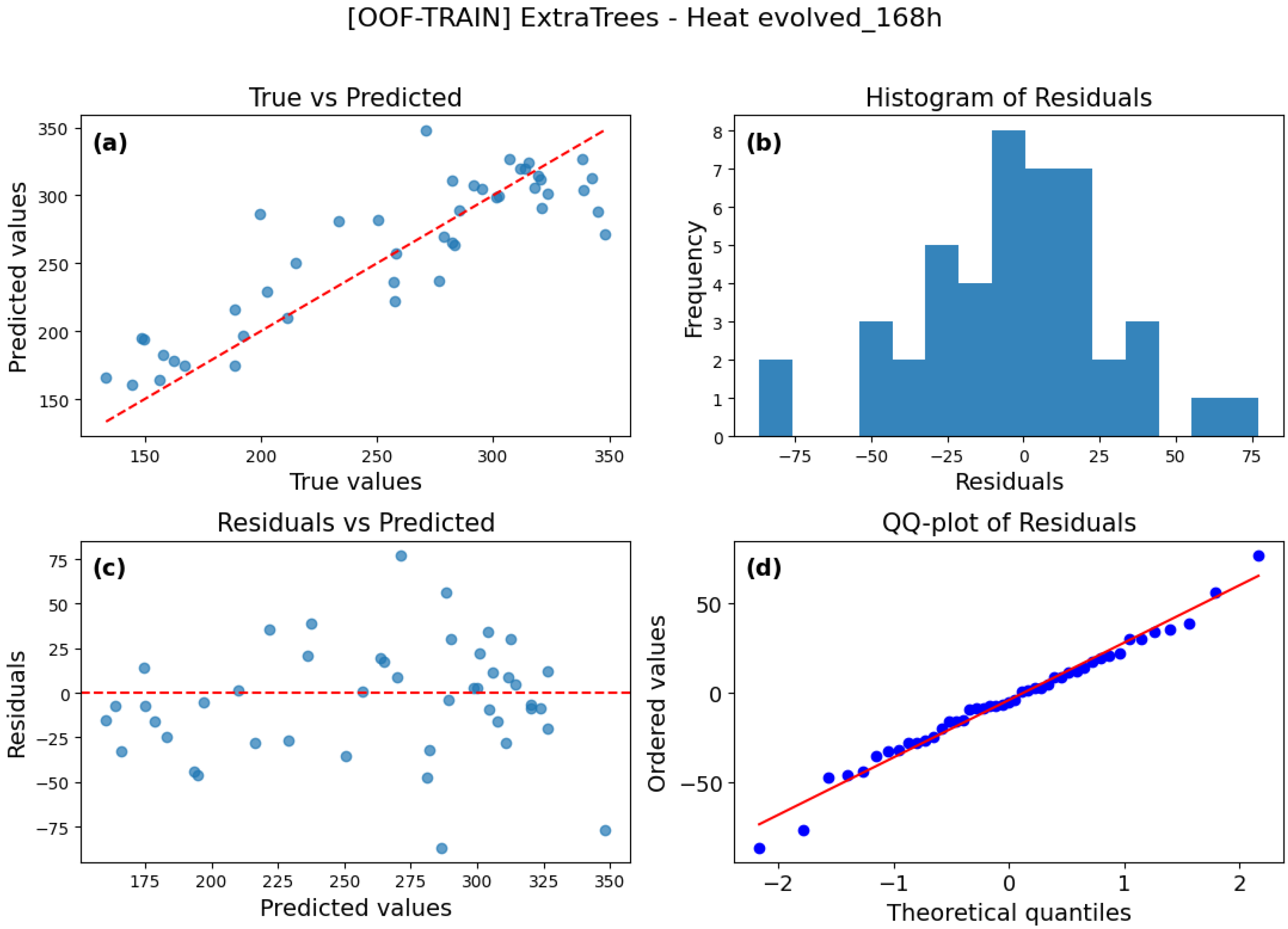
The True vs. Predicted plot (Figure 10a) shows that the ExtraTrees model captures the overall increasing trend between the true and predicted values; however, many samples display noticeable deviations from the y = x reference line. This dispersion indicates that, although the model learns the general direction and relative ordering of the data, its point-wise predictive accuracy is limited, with several predictions showing either overestimation or underestimation across the target range. The histogram of Residuals (Figure 10b) displays a largely symmetrical distribution centered around zero, with a slight predominance of negative residuals. Most residuals fall within the range of approximately −25 to +25, while only a few outliers reach values near −75 and +75. The Residuals vs. Predicted plot (Figure 10c) shows that errors remain evenly distributed around the zero axis across the entire prediction range. The distribution of residuals is relatively uniform, though a few positive and negative outliers appear at higher predicted values. The Q-Q plot (Figure 10d) indicates partial conformity of the residuals to a normal distribution in the central range, where most points align closely with the theoretical line. Deviations are visible at both distribution tails, suggesting the presence of a few extreme cases.

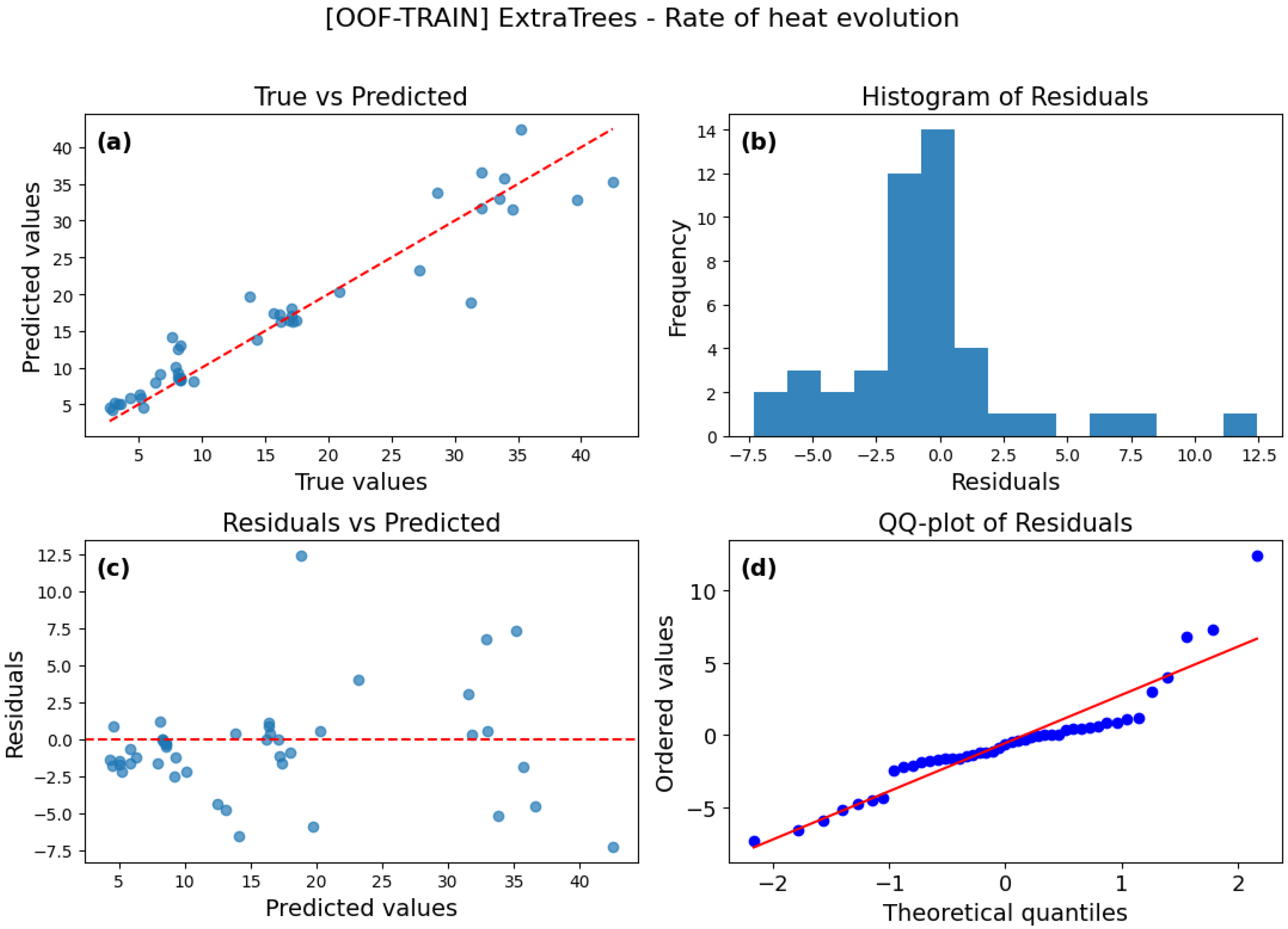
The True vs. Predicted plot (Figure 11a) for the model shows a clear linear relationship between predicted and actual values. Most points lie close to the y = x line, indicating strong agreement between predictions and observed data. Larger discrepancies appear at higher values, suggesting slightly reduced accuracy in this range. The histogram of Residuals (Figure 11b) reveals an asymmetry toward negative values, with most residuals concentrated between −2.5 and 0, forming a dominant left tail of the distribution. A few higher positive residuals (above 5) occur sporadically and may represent outliers. The Residuals vs. Predicted plot (Figure 11c) shows that residuals generally cluster around zero, confirming a good model fit. A slight increase in residual dispersion is visible for higher predicted values. The Q-Q plot (Figure 11d) indicates that the central portion of the residual distribution aligns well with the normal distribution, while deviations from the reference line appear at the extremes, particularly for the highest positive residuals.

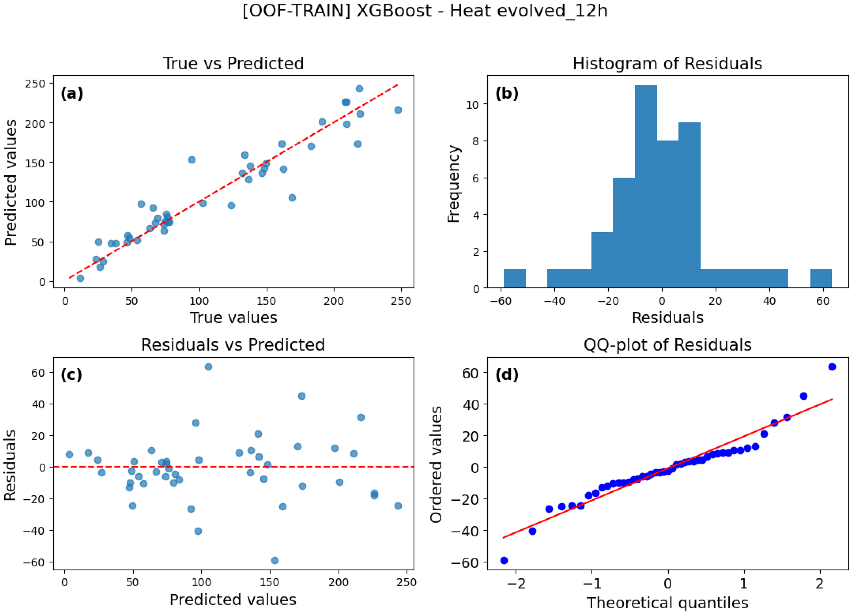
In the True vs. Predicted plot (Figure 12a) for the XGBoost model, most points lie close to the perfect-fit (y = x) line, indicating strong agreement between experimental results and model predictions. Moderate dispersion is observed, particularly at higher values, where a few points deviate further from the line. The histogram of Residuals (Figure 12b) is relatively symmetrical around zero, suggesting that the model does not exhibit a clear tendency to systematically over- or underpredict. A slight predominance of residuals near zero and slightly negative values is visible. A few isolated extreme residuals, ranging from approximately −60 to +60, indicate the presence of outliers. The Residuals vs. Predicted plot (Figure 12c) shows points evenly dispersed around the zero reference line, without a discernible systematic trend. A few larger positive and negative residuals are present, likely reflecting the inherent variability of the experimental data. The Q-Q plot (Figure 12d) demonstrates partial conformity of the residuals to a normal distribution, particularly in the central region where most points align closely with the reference line. Minor deviations at the distribution tails suggest the presence of outliers but do not significantly affect the overall goodness of fit.

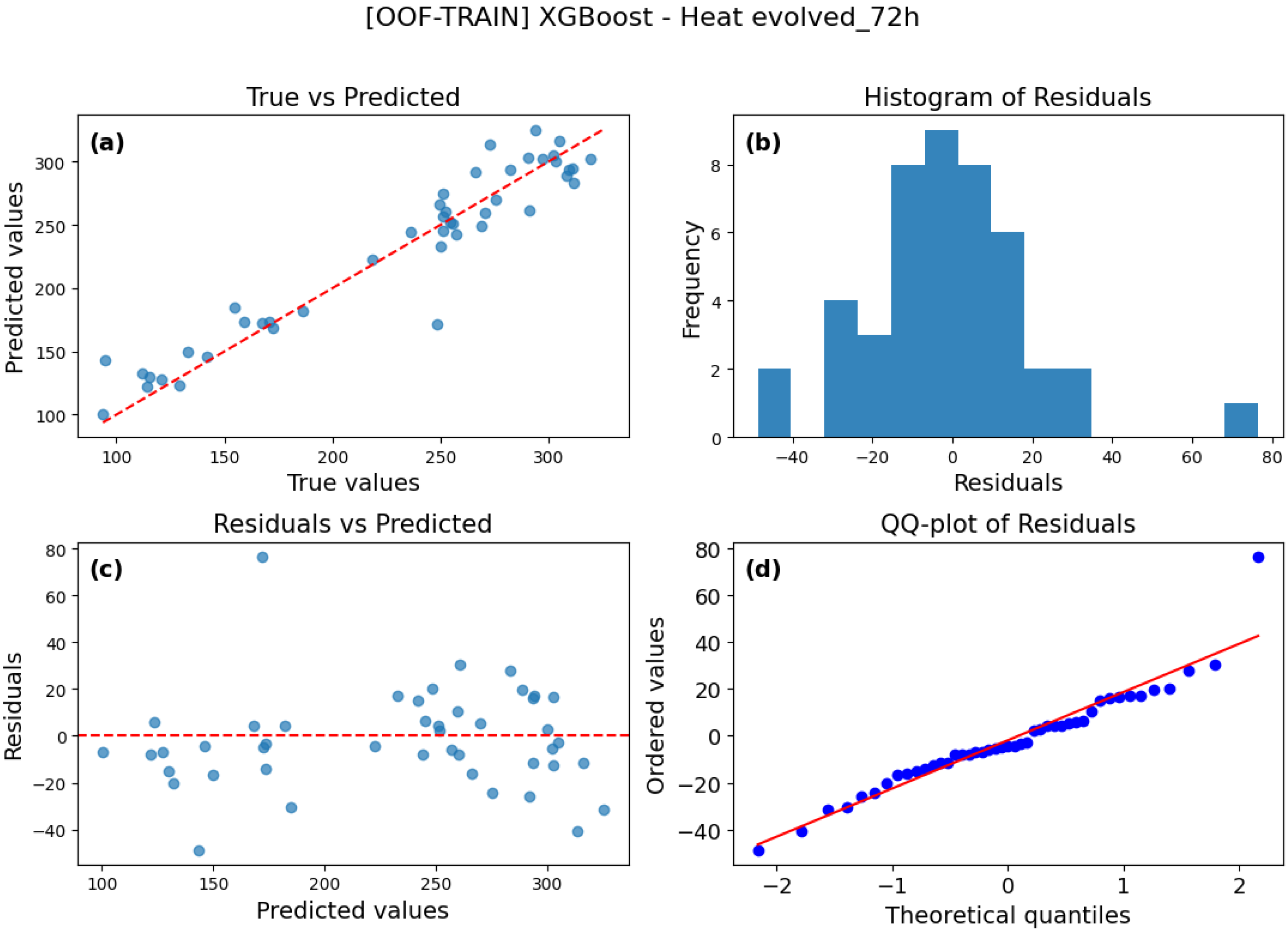
The True vs. Predicted plot (Figure 13a) for the XGBoost model shows a clear linear relationship between predicted and actual values. Most points lie close to the y = x reference line, demonstrating strong agreement between model predictions and observed data. One point deviates notably from the line, indicating a single case of greater underestimation. The histogram of Residuals (Figure 13b) displays a moderately symmetric distribution with slight asymmetry. The left tail extends to approximately −40, while the right tail reaches about +80. A single large positive residual deviates from the general trend, whereas most residuals fall within the −30 to +30 range, indicating good prediction stability. The Residuals vs. Predicted plot (Figure 13c) shows residuals dispersed around the zero axis across the full prediction range. Most residuals fall between −20 and +20, reflecting small errors and stable predictions. A few outliers are visible at both ends of the predicted range, including one significantly higher positive residual, likely attributable to natural experimental variability. The Q-Q plot (Figure 13d) shows that most points align closely with the reference line, indicating near-normal residual distribution. Deviations at the extremes suggest the presence of outliers and a slight asymmetry in the distribution.

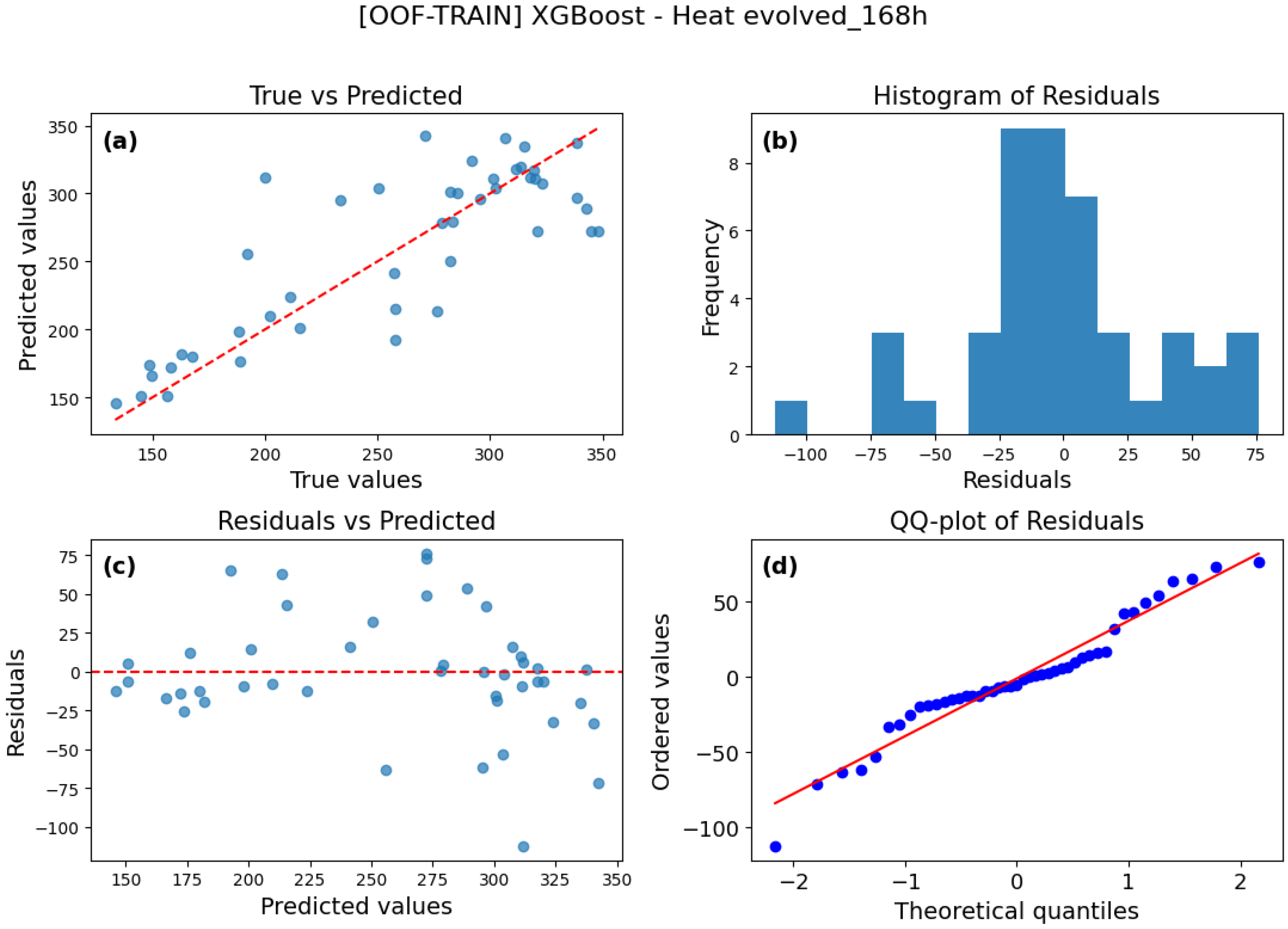
The True vs. Predicted plot (Figure 14a) for the XGBoost model shows that most points cluster near the y = x line, indicating good agreement between model predictions and observed values. The scatter of points around the line remains relatively uniform, though deviations appear at both the lower and upper ends of the range, without a clear systematic pattern of over- or underestimation. The histogram of Residuals (Figure 14b) reveals a distribution centered close to zero, with the highest concentration of residuals occurring between approximately −25 and +10. The distribution is slightly asymmetric, exhibiting a marginally longer left tail. The Residuals vs. Predicted plot (Figure 14c) shows residuals dispersed around the zero axis across the entire prediction range. Most residuals lie between −50 and +50, with a few isolated outliers at both extremes; however, no systematic spatial pattern is evident. The Q-Q plot (Figure 14d) indicates that most points align closely with the theoretical reference line, confirming near-normal residual behavior. A single point deviates markedly below the line, representing a large negative residual that may correspond to an outlier or a localized instance of model underperformance.

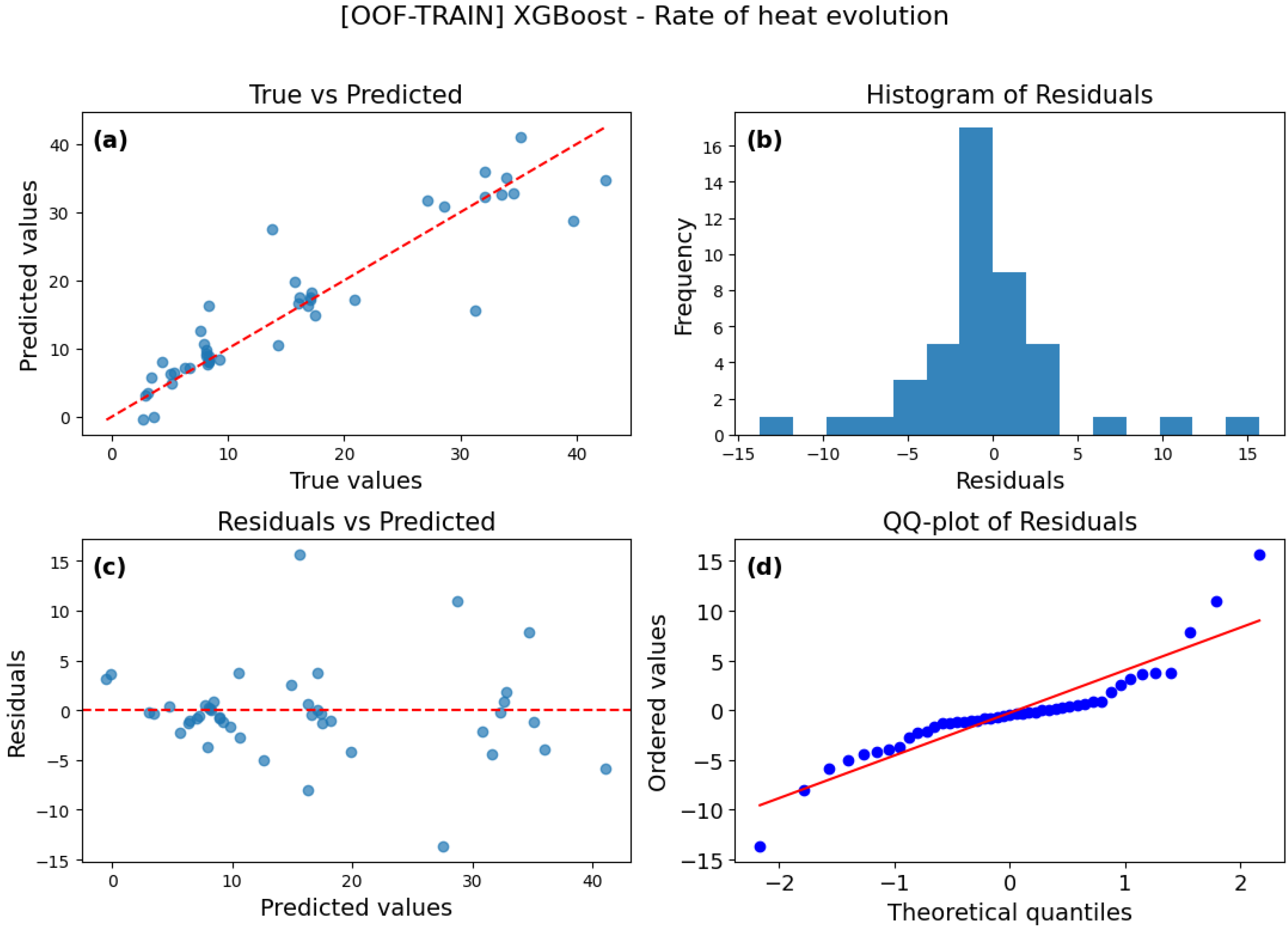
The True vs. Predicted plot (Figure 15a) shows a clear linear relationship between predicted and actual values, with points generally following the y = x reference line. This pattern indicates a good overall model fit, though a few outliers are visible, particularly at higher values. The histogram of Residuals (Figure 15b) reveals that most residuals cluster near zero, suggesting small prediction errors. A few extreme values on either side indicate occasional outliers but do not significantly affect the overall distribution. In the Residuals vs. Predicted plot (Figure 15c), residuals are distributed relatively evenly around the zero axis, with isolated deviations observed above 10 and below −10. The overall pattern suggests model stability and no clear systematic bias. The Q-Q plot (Figure 15d) shows that the central portion of the residual distribution aligns closely with the theoretical reference line, indicating approximate normality. Larger deviations appear mainly at the distribution tails for both positive and negative values, suggesting the presence of a few outliers.

3.3. Residual Diagnostics and Model Reliability Assessment

This section presents detailed statistics of the residual distributions for all models in the training set. The results include the mean and standard deviation of the residuals, the Shapiro–Wilk and D’Agostino tests for normality, and Student’s t-test for the mean of the residuals. This analysis evaluates whether the error distributions satisfy the assumptions of classical regression and identifies any potential shifts or deviations from symmetry and normality.

Table 10. Model performance TRAIN.

Model	Target	Mean Resid	Std Resid	Shapiro–Wilk p	D’Agostino p	t-Test p
CatBoost	Heat evolved (12 h)	−4.3656	16.322	0.1506	0.0244	0.0796
	Heat evolved (72 h)	−6.3195	24.888	0.345	0.0729	0.0956
	Heat evolved (168 h)	−5.161	35.597	0.7564	0.3785	0.3361
	Rate of heat evolution	−0.7565	3.7024	0.0007	0.0001	0.1774
ExtraTrees	Heat evolved (12 h)	−3.589	15.534	0.1384	0.0383	0.1283
	Heat evolved (72 h)	−5.2971	20.518	0.7813	0.3994	0.0903
	Heat evolved (168 h)	−4.0489	31.683	0.8486	0.4102	0.3959
	Rate of heat evolution	−0.555	3.4835	0.0002	0.0001	0.291
XGBoost	Heat evolved (12 h)	−1.1269	20.419	0.0333	0.0274	0.713
	Heat evolved (72 h)	−1.8919	20.885	0.0171	0.0008	0.5465
	Heat evolved (168 h)	−1.3077	38.109	0.0728	0.3266	0.819
	Rate of heat evolution	0.3361	4.5178	0.0002	0.0006	0.6878

presents key diagnostic statistics for the CatBoost, ExtraTrees, and XGBoost models used to predict the four target variables: heat evolved (12 h, 72 h, and 168 h) and rate of heat evolution. For all models, the mean residuals for heat evolved (12 h, 72 h, 168 h) are negative, indicating a slight tendency to underestimate the target values. Among them, XGBoost consistently produces the smallest (least negative) mean residuals across all time periods, suggesting superior bias control. For the rate of heat evolution, XGBoost also achieves the mean value closest to zero. The standard deviation of residuals for heat evolved increases with the time horizon across all models, reflecting growing error variability with larger target values-a typical behavior in regression problems. Among the three models, ExtraTrees achieved the lowest standard deviations for all heat evolved variables. Similarly, for rate of heat evolution, all models showed lower variability overall, with ExtraTrees again achieving the lowest value. Results of the Shapiro–Wilk and D’Agostino normality tests indicate that, in several cases, the residual distributions deviate from normality (p < 0.05), leading to rejection of the normality hypothesis. Cases where p > 0.05—indicating no significant deviation from normality—include: CatBoost for heat evolved 72 h and 168 h (2 of 4 variables), ExtraTrees for heat evolved 72 h and 168 h (2 of 4), and XGBoost for heat evolved 168 h (1 of 4). The non-normal distributions observed for rate of heat evolution and heat evolved 12 h across all models may stem from asymmetry, long tails, or heteroscedasticity effects. Results of Student’s t-test for the mean of residuals revealed no significant bias across models (p > 0.05 for all 12 cases). XGBoost demonstrated the highest consistency in this regard (p = 0.55–0.82), indicating the greatest stability and lack of systematic bias. CatBoost for heat evolved 12 h and 72 h, and ExtraTrees for heat evolved 72 h, exhibited p-values closest to the significance threshold.

3.4. Test Set Performance Metrics for Each Model and Target

This section presents the performance metrics obtained by the models on an independent test set. The evaluated metrics include the mean absolute error (MAE), root mean square error (RMSE), mean absolute percentage error (MAPE), and coefficient of determination (R²), calculated for the CatBoost, ExtraTrees, and XGBoost models across all four target variables. These results enable a direct comparison of the predictive performance of the individual algorithms and allow for identifying which model achieves the lowest prediction error based on the given output data.

The lowest MAE values (

Table 11. Model performance using MAE per target and model (TEST).

	Model	CatBoost	ExtraTrees	XGBoost
Target
Heat evolved (12 h)		8.622	8.544	7.849
Heat evolved (72 h)		8.976	11.264	8.950
Heat evolved (168 h)		17.233	17.029	17.324
Rate of heat evolution		1.368	0.895	1.497

) for the test set were achieved by XGBoost for the short-term heat evolved forecasts at 12 h and 72 h. ExtraTrees performed best for the long-term heat evolved predictions at 168 h and for the rate of heat evolution. The CatBoost results for most variables are comparable to those of ExtraTrees and XGBoost, indicating similar predictive performance. Overall, ExtraTrees achieved the lowest absolute errors for rate of heat evolution and heat evolved (168 h)-though only marginally lower than the other models-while XGBoost provided the most accurate predictions for the short-term heat evolved (12 h and 72 h) horizons.

Table 12. Model performance using RMSE per target and model (TEST).

	Model	CatBoost	ExtraTrees	XGBoost
Target
Heat evolved (12 h)		11.460	10.607	10.432
Heat evolved (72 h)		11.163	12.528	10.300
Heat evolved (168 h)		19.679	20.837	21.359
Rate of heat evolution		1.680	1.055	1.842

presents the RMSE values obtained by the models. Based on the test data, XGBoost achieved the lowest errors for heat evolved predictions at 12 h and 72 h, while CatBoost performed best for the 168 h horizon, yielding a lower RMSE than both ExtraTrees and XGBoost. In contrast, ExtraTrees clearly outperformed the other models for the rate of heat evolution, achieving the lowest error in this category. Each model demonstrates specific strengths, with overall performance remaining comparable across short- and medium-term horizons. However, ExtraTrees shows superior precision when predicting the heat release rate.

A comparison of the MAPE values (

Table 13. Model performance using MAPE per target and model (TEST).

	Model	CatBoost	ExtraTrees	XGBoost
Target
Heat evolved (12 h)		0.100	0.091	0.105
Heat evolved (72 h)		0.043	0.055	0.047
Heat evolved (168 h)		0.071	0.068	0.070
Rate of heat evolution		0.124	0.095	0.155

) for the test data shows that ExtraTrees achieved the lowest percentage errors for heat evolved after 12 h and for the rate of heat evolution, indicating superior relative accuracy in these tasks. CatBoost slightly outperformed the other models in predicting heat evolved after 72 h. XGBoost obtained the best result only for heat evolved at 72 h, while in other cases its MAPE values were higher, particularly for the rate of heat evolution, suggesting greater sensitivity to individual outliers in this task. Overall, ExtraTrees demonstrates the most consistent relative accuracy across targets, whereas XGBoost shows more variable performance depending on the predicted feature.

A comparison of the R² values on the test set (

Table 14. Model performance using R² per target and model (TEST).

	Model	CatBoost	ExtraTrees	XGBoost
Target
Heat evolved (12 h)		0.965	0.970	0.971
Heat evolved (72 h)		0.957	0.946	0.964
Heat evolved (168 h)		0.822	0.800	0.790
Rate of heat evolution		0.973	0.989	0.967

) shows that all models achieved a very high degree of fit for the short-term heat evolved predictions at 12 h and 72 h, as well as for the rate of heat evolution, with R² values exceeding 0.94 in each case. This indicates excellent agreement between the model predictions and the observed data. XGBoost achieved the highest R² values for heat evolved at 12 h and 72 h, CatBoost performed best for the long-term heat evolved at 168 h, and ExtraTrees showed the best performance for the rate of heat evolution (R² = 0.989). The largest differences among models are observed for the long-term prediction horizon. The moderate reduction in R² observed for the 168 h horizon can be attributed to the cumulative nature of long-term heat evolution, which naturally increases variability and makes later-age values more challenging to model accurately compared with short-term measurements. Moreover, the limited dataset size contributes to higher variance in the estimated model fit, which is reflected in the lower R² relative to earlier prediction horizons [46]. Nevertheless, the obtained R² values of approximately 0.79–0.82 indicate that the models still maintain a reasonable level of explanatory power for long-term heat evolution. Overall, all algorithms exhibit very strong fits to the test data for short-term horizons and for heat release rate prediction, while CatBoost demonstrates the highest goodness of fit for long-term forecasts.

3.5. Sample-Wise Diagnostic Evaluation on the Test Set

This section presents an evaluation of prediction errors for individual samples in the independent test set, using residual plots and predicted-versus-actual value comparisons.

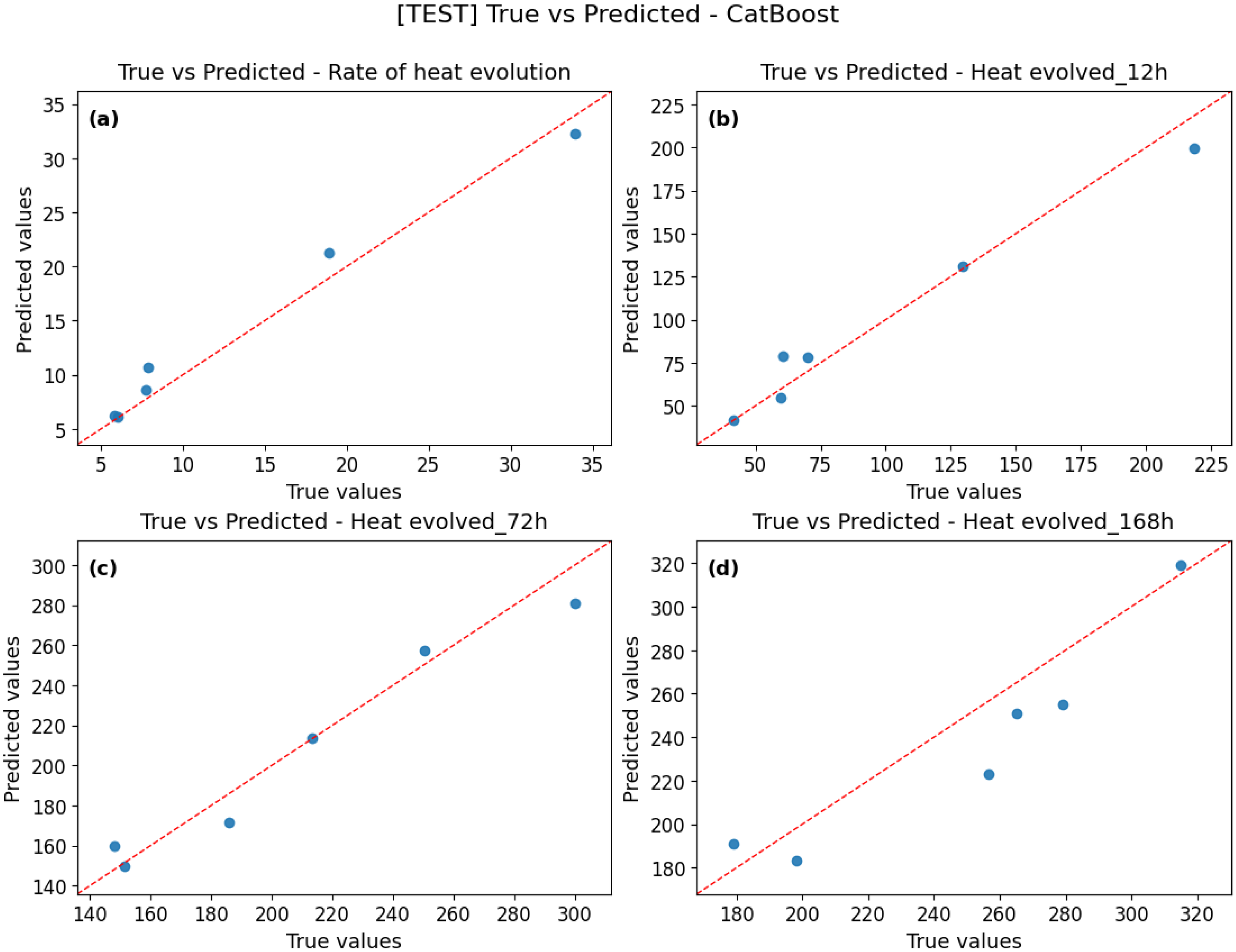
The True vs. Predicted plots (Figure 16) for the CatBoost model on the test set illustrate the accuracy of individual predictions for the four output parameters. For rate of heat evolution (Figure 16a), heat evolved 12 h (Figure 16b), and heat evolved 72 h (Figure 16c), the predictions align closely with the line of perfect fit (y = x), indicating high model precision relative to the actual values. For heat evolved 168 h (Figure 16d), a noticeable increase in dispersion is observed; points within the ~240–300 range systematically fall below the y = x line, indicating a tendency to underestimate values in the mid-to-upper range. Despite the extended prediction horizon, no sample shows a substantial deviation or a clearly erroneous prediction. Overall, the plots demonstrate a strong fit of the CatBoost model to the test data, reflecting stable predictive performance which is characterized by smaller errors for short-term forecasts and consistent accuracy even in more challenging, long-term cases.

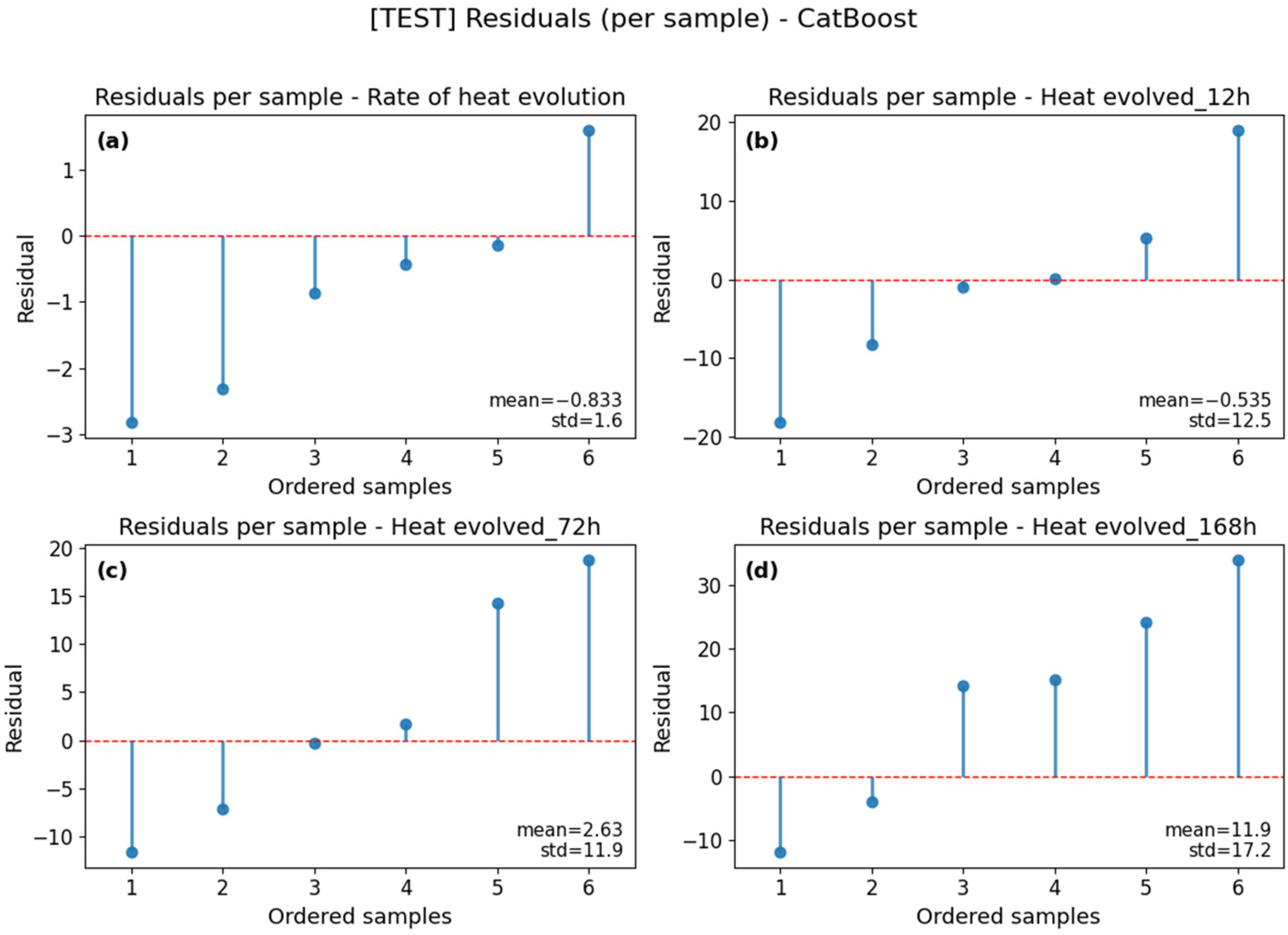
The residual plots for the CatBoost model (Figure 17) illustrate the distribution of prediction errors for each test sample across the four output parameters. For the rate of heat evolution (Figure 17a), the residuals are distributed on both sides of zero, with several samples showing deviations of approximately 1.5–3 units. These values indicate noticeable variation in point-wise prediction accuracy, which is also reflected in the mean (−0.83) and standard deviation (1.6). For heat evolved (12 h) (Figure 17b), errors are evenly distributed (mean −0.54; SD 12.5), although two residuals deviate noticeably from zero. At longer prediction horizons heat evolved (72 h) (Figure 17c) and heat evolved (168 h) (Figure 17d) greater error variability is evident, with mean and standard deviation increasing to 2.63/11.9 and 11.9/17.2, respectively. This pattern indicates wider residual scatter and the emergence of a few extreme error values. Overall, CatBoost demonstrates stable and accurate predictions for short-term forecasts, while error magnitudes increase moderately for longer horizons.

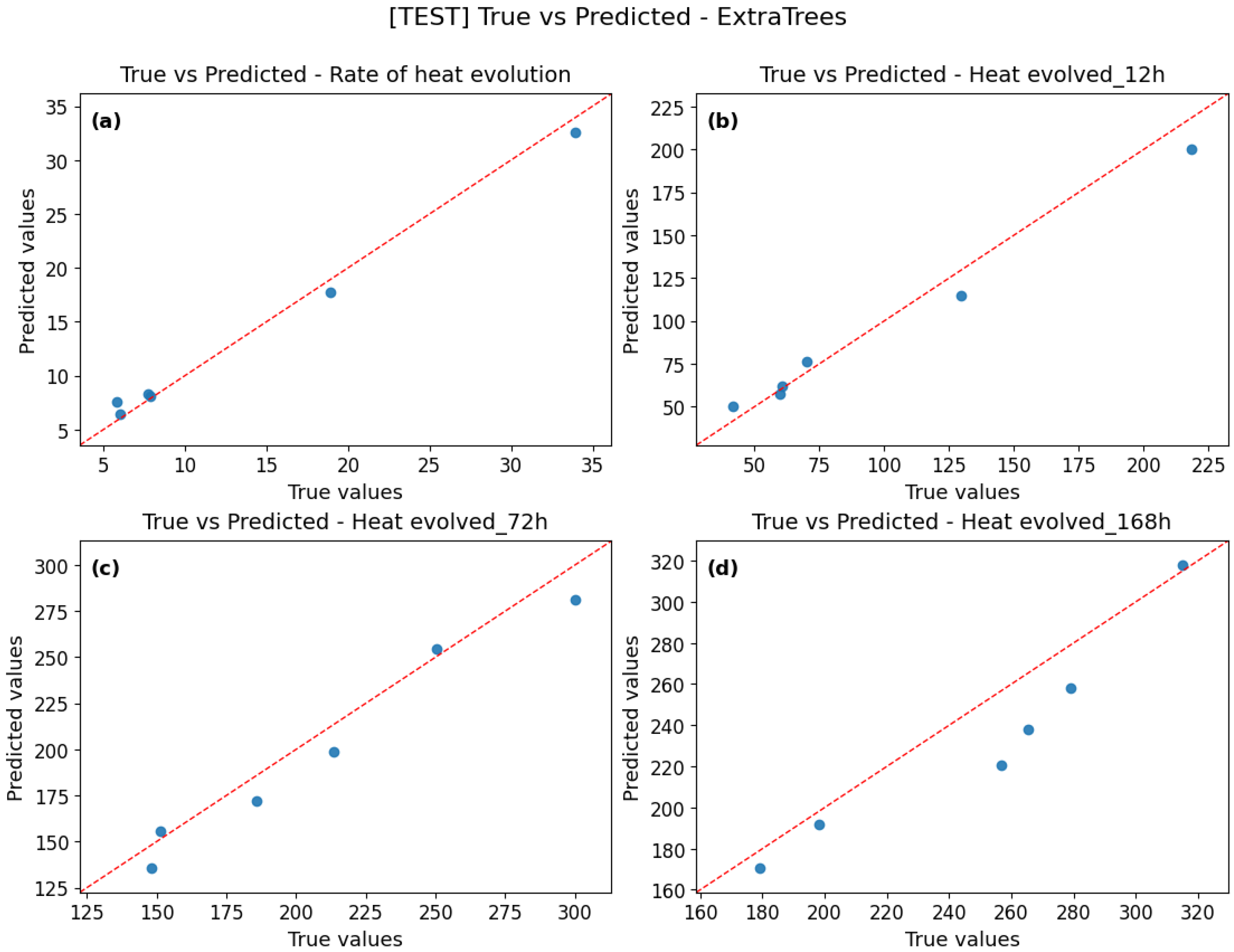
Figure 18 compares the values predicted by the ExtraTrees model with the actual observations from the test set for the parameters heat evolved (12 h, 72 h, and 168 h) and rate of heat evolution. In each plot, the points represent individual test samples and are plotted against the line of perfect fit (y = x). Analysis of the point distributions relative to this line shows that for rate of heat evolution (Figure 18a), heat evolved 12 h (Figure 18b), and heat evolved 72 h (Figure 18c), most predictions closely match the actual values. In contrast, for heat evolved 168 h (Figure 18d), a broader scatter and a tendency toward increased forecast dispersion are observed. The distance of the points from the line of perfect fit indicates a gradual increase in individual prediction errors with longer time horizons. No dataset exhibits significant outliers, and the model maintains predictions within reasonable limits. However, the extended forecast horizon (168 h) is associated with larger error amplitudes and slight systematic deviations at higher reference values. Overall, the analysis confirms that the ExtraTrees model maintains high predictive accuracy for short-term horizons, while error dispersion becomes more pronounced in long-term forecasts.

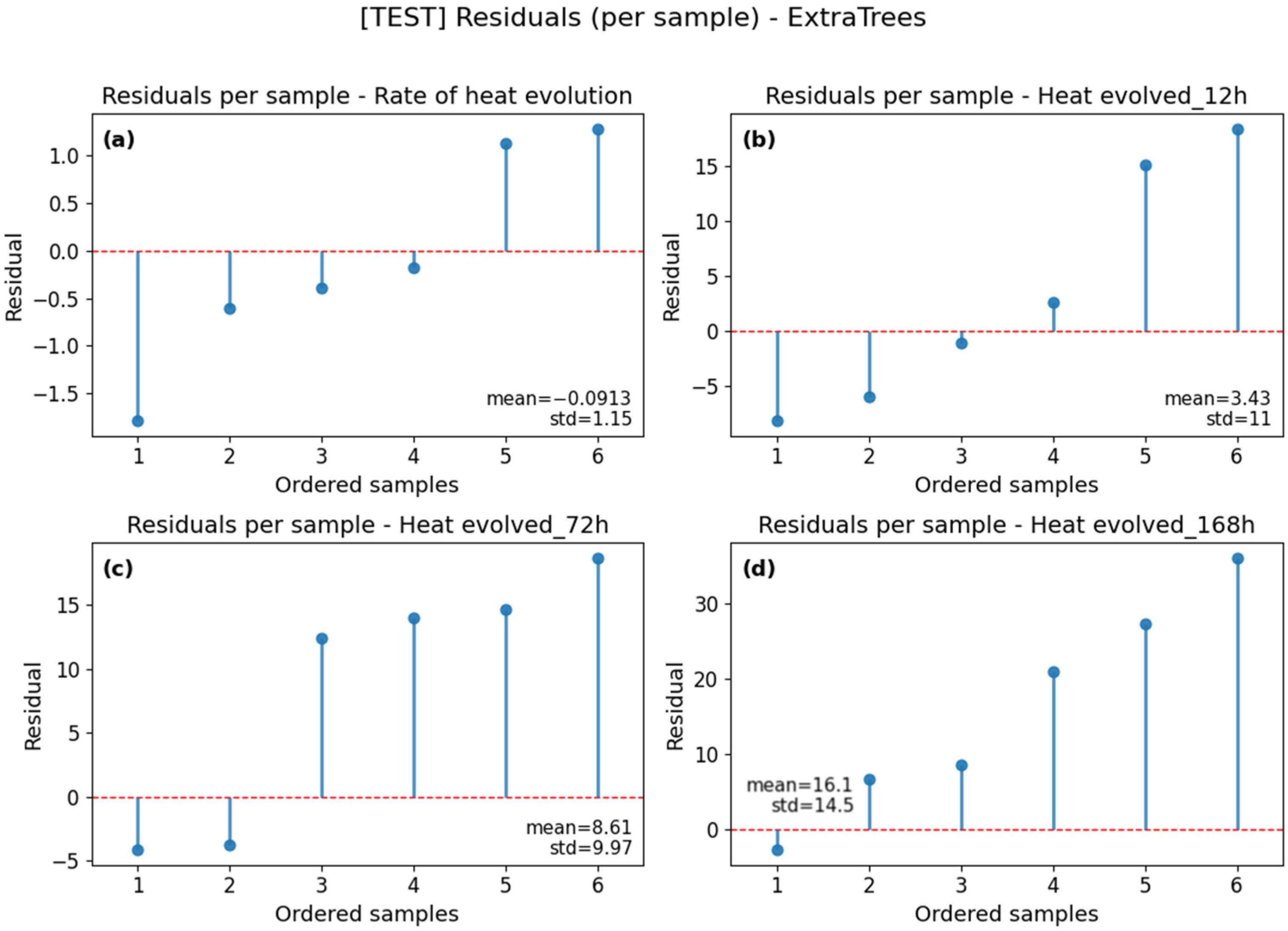
The residual plots for the ExtraTrees model (Figure 19) illustrate the individual prediction errors for each sample in the test set, shown separately for heat evolved after 12, 72, and 168 h, and for the rate of heat evolution. For the rate of heat evolution (Figure 19a), most residuals are concentrated near zero, exhibiting moderate variability and only a few deviations exceeding one unit. The mean (−0.09) and standard deviation (1.15) confirm the excellent stability of the model in this task. For heat evolved after 12 h (Figure 19b), errors remain relatively small (mean 3.43, SD 11.0), although two more pronounced deviations are observed. As the time horizon increases to 72 h (Figure 19c) and 168 h (Figure 19d), the residual scatter widens, with mean shifts of 8.6 (SD 9.97) and 16.4 (SD 14.5), respectively, and more noticeable outliers appearing. The progressive increase in residual dispersion with longer prediction horizons reflects the typical decline in model stability over time. Overall, the analysis indicates that the ExtraTrees model exhibits high stability and accuracy for predicting the rate of heat evolution and short-term heat evolved values. However, for longer horizons, the systematic increase in errors suggests a need for further model optimization and investigation of potential outliers or atypical input cases.

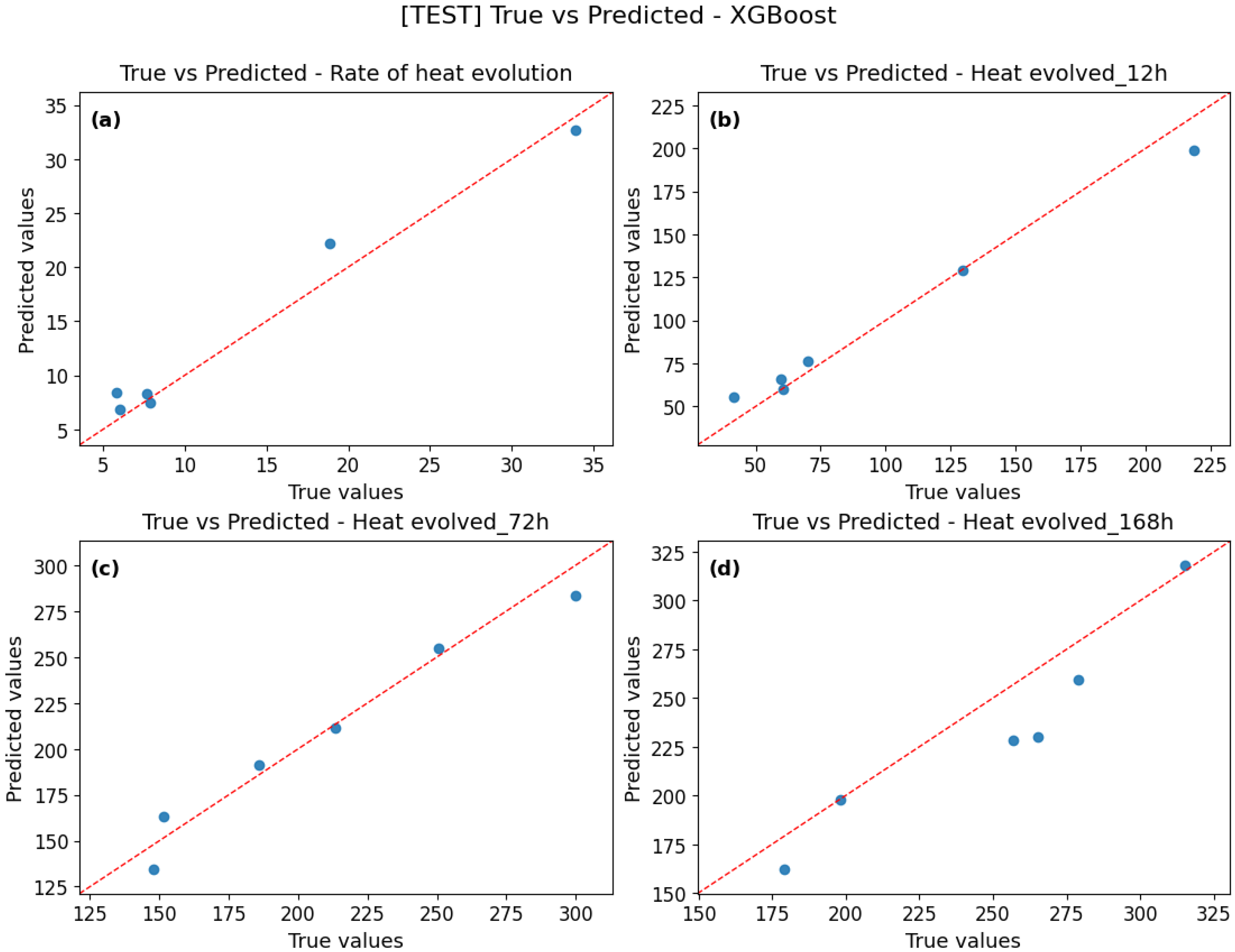
The True vs. Predicted plots (Figure 20) for the XGBoost model show that the predictions generally follow the increasing trend of the observed values across all four output variables. While several points align reasonably well with the y = x reference line, other samples exhibit noticeable deviations, indicating variability in point-wise predictive accuracy. Overall, the model captures the global relationship between true and predicted values, but individual test samples display moderate dispersion around the line of perfect agreement. Predictions for rate of heat evolution (Figure 20a), heat evolved 12 h (Figure 20b), and heat evolved 72 h (Figure 20c) align particularly well with the reference line, while for heat evolved 168 h (Figure 20d), a slightly larger scatter is observed, though the overall distribution remains consistent. Minor underestimations and overestimations appear mainly at the extreme values. Overall, the analysis confirms that XGBoost achieves strong predictive accuracy and stability across all targets.

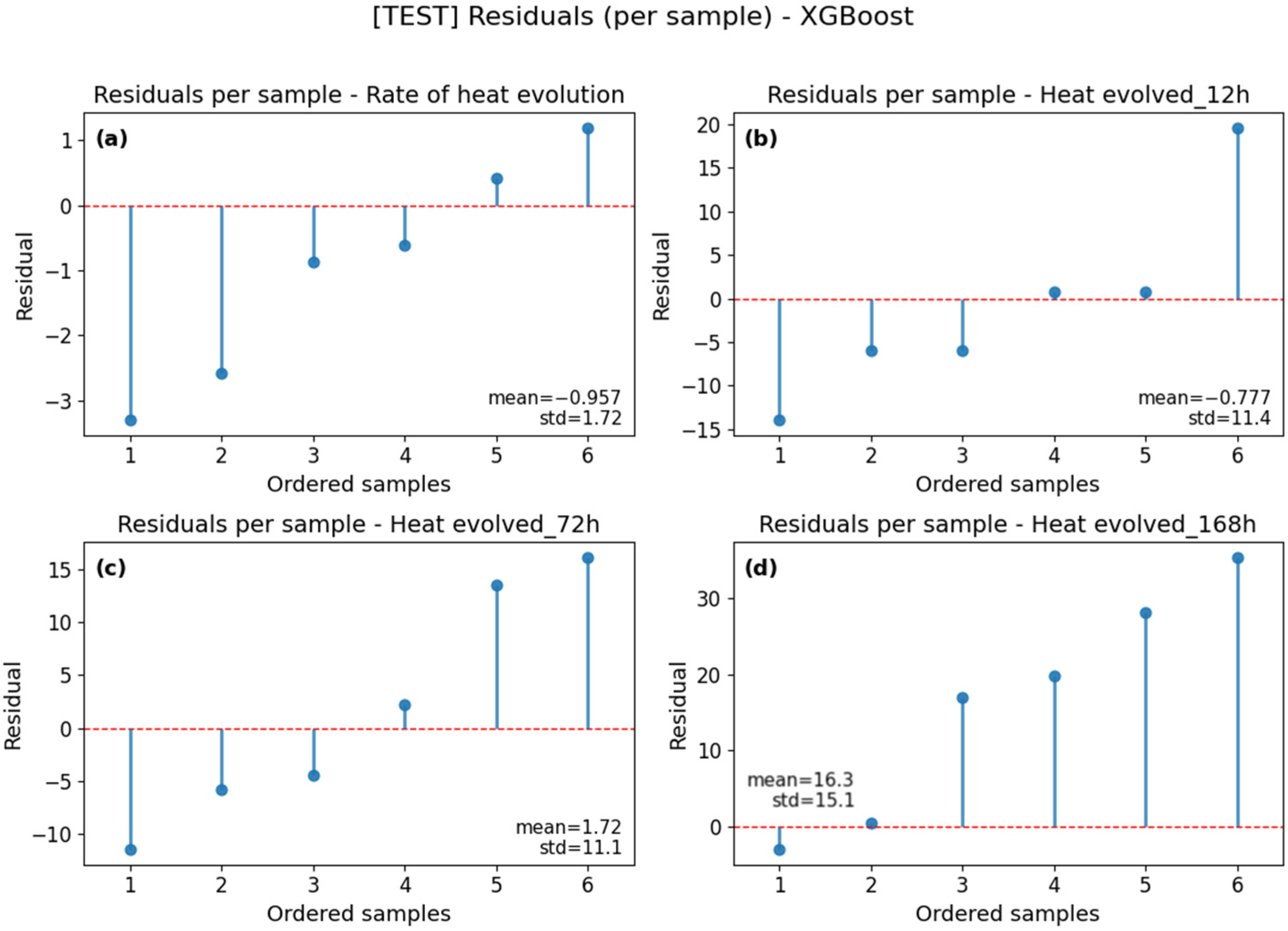
The residual plots for the XGBoost model illustrate the distribution of prediction errors for each test sample across the four target variables. For the rate of heat evolution (Figure 21a), the residuals are concentrated near zero (mean −0.96, variance 1.72), indicating strong model stability. The results for heat evolved 12 h (Figure 21b), also show relatively low residual scatter (mean −0.78, SD 11.4), with only a single markedly positive outlier. At the 72 h horizon (Figure 21c), (mean 1.72, SD 11.1), a slight underestimation trend is observed, though the overall error distribution remains moderate. For heat evolved 168 h (Figure 21d), a distinct positive bias appears (mean 16.3, SD 15.1), along with several large positive residuals, suggesting systematic underestimation at longer time horizons. Overall, the XGBoost model demonstrates high stability and low error levels for short-term predictions but exhibits an increasing susceptibility to higher errors and systematic positive bias in long-term forecasts, particularly for the most demanding test cases.

4. Conclusions

A comparative analysis of three machine learning models, CatBoost, ExtraTrees, and XGBoost, for predicting the evolution of hydration heat and the heat release rate demonstrated that all algorithms achieved high prediction accuracy. Model performance was evaluated using multiple error metrics (MAE, RMSE, MAPE) and the coefficient of determination (R²), complemented by residual analysis and statistical tests assessing the distribution and unbiasedness of errors.

The following section outlines the performance of the three evaluated models, with attention to their accuracy, stability, and error characteristics, while acknowledging that the reported results may depend on the specific dataset and experimental conditions:

• The ExtraTrees model exhibited the most stable and consistent performance among the tested algorithms. On the training set, it achieved the lowest MAE and RMSE values in most cases, particularly for long-term prediction horizons (168 h). It also showed the lowest standard deviations across all variables and no significant systematic deviations, as confirmed by Student’s t-tests (p > 0.05). Its superiority can be attributed to the effective aggregation of decision trees, which enhances model generalization and mitigates overfitting.
• The XGBoost model delivered the highest accuracy for short-term predictions of cumulative heat evolved after 72 h, achieving the lowest MAE and RMSE values and the highest R² (up to 0.971). These results confirm the algorithm’s strong capability to capture the dynamics of the early hydration stages. However, as the prediction horizon increased, the model exhibited growing asymmetry in the residual distribution, suggesting declining stability over longer periods.
• The CatBoost model produced results comparable to those of the other two algorithms, though slightly inferior in some cases. Despite showing greater variability in short-term residuals, CatBoost maintained relatively low relative errors and good overall prediction stability. Residual diagnostics indicated that, for most models, error distributions were approximately normal within the central range. Nonetheless, deviations from normality were observed for shorter time horizons and for the rate of heat evolution variable, caused by distribution asymmetry and the presence of outliers. The absence of significant mean residual shifts confirmed the lack of systematic prediction bias. The observed increase in error variance with longer time horizons reflects the typical accumulation of uncertainty in regression models.
• Evaluation on the independent test set confirmed the high generalization ability of all three models. For short-term predictions (12–72 h), all algorithms achieved R² values exceeding 0.94, while for long-term predictions (168 h), a moderate decline in accuracy was observed (R² ≈ 0.8). This decrease may be attributed to the cumulative nature of long-term heat evolution, which naturally increases variability, and further validation on a larger dataset would be required to clarify this effect. The best fit was obtained for the rate of heat evolution variable (R² = 0.989, ExtraTrees), highlighting the potential of this model to accurately represent hydration processes.

Overall, the results indicate that no single model consistently outperforms the others across all timescales. Therefore, the choice of algorithm should be guided by the characteristics of the predicted phenomenon and the target time horizon. The findings confirm the suitability of ensemble learning methods for modeling hydration processes and emphasize the importance of further research on hyperparameter optimization and hybrid model integration to simultaneously enhance accuracy and interpretability.

Future work should also focus on expanding the training dataset to include diverse experimental conditions and material compositions, which would improve the models’ generalization capabilities and robustness in predicting hydration behavior across a broader range of scenarios.