Current-Flux Plane Sliding Mode for Induction Motor Torque Control

Abstract

The induction motors are once again becoming increasingly more popular due to the shifts in global politics and economics. With this increased interest, there is a growing need for even better control solutions, especially for the automotive industry, which requires high safety standars. This study presents a new sliding mode control method for induction motor torque control that aims to accelerate the flux dynamics response and grant robustness. The method employs two sliding mode controllers, one for each of the dq-frame axes. The q-axis is controlled with a well-known time-varying sliding mode to ensure rapid response of the system. The d-axis is controlled with a sliding mode employing both current and flux error values in order to decrease d-axis flux time constant. The proposed method is analyzed theoretically, and the obtained results are confronted with the practical results obtained through experiments on a typical induction machine.

1. Introduction

Sliding mode control (SMC) belongs to the class of variable structure methods. The controllers designed according to it force the state trajectory to ‘slide’ along a predefined subspace of the state space. This subspace has a reduced dimension therefore, once the sliding motion is enforced, the order of the system is decreased, simplifying its dynamics. What is more, during this motion, the system is completely insensitive to the so-called matched disturbances, that act on the state in the same ‘direction’ as the control signal. An additional advantage of sliding mode controllers is the relative simplicity of their equations, enabling short computations, which is important for fast-acting control loops. The theoretical groundwork of sliding mode control was laid out quite some time ago; however, due to the practical advantages stated above, the approach is still being developed and used presently.

Because of the inherently discontinuous nature of the control signal, sliding modes are often employed in power converter and electric drive systems [1,2,3]; as in these applications, the control signal (semiconductor switch state) is on its own not continuous. One of the aspects of practical implementation of sliding mode control is ensuring a-priori known bounds on the control signal and states of the system [4]. This is obviously important in real systems as, e.g., speed, electrical currents, etc., must be limited to prevent damage and ensure safe operation. In [5] the authors developed a sliding mode controller for a linear servomechanism; unfortunately only the input constraint was guaranteed. The authors of [6] proposed an adaptive neural network nonsingular sliding mode controller for a linear permanent magnet synchronous motor (PMSM). The principal problem in such a control task are the unknown and possibly position-varying parameters of the motor. The neural network estimates the motor parameters on-line and the adaptive part ’fine-tunes’ the discontinuous part of the control signal to minimize chattering while still ensuring robustness. Sliding mode control of a linear PMSM was also considered in [7,8].

One of the novel power converter systems is the neutral point clamped (NPC) converter. Such a converter can form the output voltage from more “levels” than a typical converter, which in general terms improves the power efficiency (due to lower harmonic distortion, good quality of output waveforms, etc.). In [9] an adaptive super-twisting sliding mode controller is used in the power control loop. Moreover, a disturbance observer-based strategy maintains the dc-link voltage, and a PI controller ensures balance between the two dc-link capacitors voltage. Simulations and experimental results confirm the improvement in harmonic distortion of the waveforms (caused by a reduction in chattering) and the disturbance rejection capabilities of the proposed controller. A similar problem is considered in [10], where a finite time sliding mode controller is used to further reduce the regulation time.

Another novelty in sliding mode systems is utilizing the barrier function approach, which was used in [11] to control a supply chain model. In this method, one of the gains of the super-twisting sliding mode controller is increased until the state reaches a vicinity of the switching manifold (to ensure rapid convergence) and then is decreased. It is then demonstrated that this modification allows it to outperform both $H_{\infty }$ control as well as a terminal sliding mode controller in terms of convergence speed and chattering elimination. A super-twisting sliding mode controller was also used in [12] for a hydraulic excavator system. The controller utilizes a fractional order sliding hyperplane to improve transient performance and minimize steady state error. Computer simulations confirm that this approach outperforms both the terminal sliding mode controller as well as the adaptive fuzzy sliding mode one in terms of control precision and chattering reduction.

As was already stated, the major benefits of sliding mode control are guaranteed only from the start of the sliding motion. Typically, when one selects the sliding hyperplane to obtain the best system dynamics, the initial state is not positioned on it. Thus, at the start of the control process, the robustness is not ensured. To deal with this problem, two main approaches exist: reaching laws [13] and time-varying sliding hyperplanes [14]. In this work, the second one will be used. It relies on translating and/or rotating the sliding hyperplane so that it first passes through the initial state, and after some predetermined time it crosses the desired state. If this is done properly, the sliding motion, along with its advantages, can be maintained from the very start of the controller operation.

In [15], a time varying sliding line is used to control an uninterruptible power supply (UPS). The error of the output voltage affects the rotation of the sliding line. When this error is large, the line becomes more ‘steep’, which results in rapid convergence toward the desired voltage. On the other hand, when this error is small, the line gets less ‘steep’ so that chattering in the vicinity of the desired voltage is reduced. These results were then confirmed in laboratory tests [16].

Some time-varying SMC strategies are also used for induction motor (IM) control. Recently, these machines have again become popular, after a period of PMSM dominance. Regardless of the higher power density of the PMSM, more and more drives are being created with the IMs. This is visible especially in the automotive industry and is caused by currently occurring changes in the global economy [17,18,19,20,21,22,23].

Similarly to PMSMs, speed control time-varying sliding modes [24] are considered most commonly in case of the IMs. Similar approach to current or torque control is rare. An important issue when it comes to the IM current control is that it is a first-order system. Since the use of the SMC reduces the system dimension, the resulting control happens in a one-dimensional state space. Therefore, the time-varying SMC strategies are not that popular in this case. Nevertheless, one approach to this problem was presented in [25].

Comparing PMSMs and IMs, torque control is significantly easier for the first type of machines due to the constant flux ensured by permanent magnets. It is fairly frequent to use field-oriented control (FOC) with dq-frame transformation for both mentioned types of machines. If this is the case, the PMSM torque is generated by controlling only the q-axis current, while keeping d-axis current equal to zero (except in some specific scenarios). In the case of the IM, the torque control problem is more complex as the rotor flux must be generated by the d-axis current, and the torque value is proportional to the cross product of the rotor flux vector and the stator current vector. Therefore, especially when the IM startup is considered, it is more time-consuming to generate IM torque than PMSM torque.

Direct torque control (DTC) is a control method renowned for its robustness and speed of operation. In [26] the authors have shown that both FOC and DTC give similar results for PMSMs. However, when the IM is considered, DTC is superior to FOC in a certain way, due to the shape of torque response [27], which is linear-like in case of DTC and aperiodic for FOC. It was first proposed in [28]. Over the years, many articles suggested the use SMC-based DTC. One example can be found in [29], where the authors presented a method for sensorless IM speed control employing cascade control structure with sliding mode torque controller.

In [30] the authors performed a particular IM state transformation to use flux magnitude and torque value as state variables. Then they proposed two sliding manifolds, one for flux magnitude control and the other for torque value control. Both sliding manifolds were designed for first-order systems; hence, the SMC was reduced to a point. Authors showed that by quantizing the resulting control voltages, the DTC switching table identical to the one presented in [28] is obtained. Therefore, the DTC was analytically proven to be a special case of the SMC.

Rapid torque control provided with DTC does not come without a price, as the transient current response is characterized with significant overshoot. There are in fact more disadvantages to DTC; however, the key point is that in the case of the IM torque control, one must always choose between faster torque convergence and limiting the current response. For this reason, some methods for limiting current response obtained with DTC were proposed [31,32].

The recent literature shows a shift toward more advanced techniques, including space-vector-modulated DTC, model-predictive torque control (MPTC), adaptive and robust FOC variants, and sensorless estimation methods, that enhance performance under parameter variations [33,34,35]. Increasingly, researchers are also exploring AI-assisted approaches, such as neural-network-based observers and reinforcement-learning torque controllers. This shows that there is a growing need for robust and reliable torque control methods.

In this paper we propose a new definition of a sliding manifold to allow for compromise between current overshoot and flux convergence time constant. The structure of the paper is organized as follows:

• The induction motor model is introduced in the Preliminaries section, and it is shown how d- and q-axis control voltages are decoupled. The main idea behind the proposed control method is also described.
• The q-axis current, which impacts the torque value, is controlled independently of the d-axis dynamics with use of the time-varying sliding mode designed in the next section.
• Later, the d-axis current-flux plain sliding mode controller is designed and analyzed. It is shown how the sliding mode parameters affect the flux convergence rate.
• Practical results are presented in the Experimental Results section, where laboratory setup and test conditions are described. Several tests for various scenarios are conducted. It is shown that the induction motor controller with the proposed method behaves as predicted with the theoretical analysis.

The presented approach implies that the torque control performance is determined almost entirely on the d-axis flux dynamics. Moreover, the current limitation is embedded into the proposed strategy, and no additional current limitation strategy is required. The proposed control system is thoroughly analyzed to show its characteristics, for instance, how the maximum value of the d-axis current depends on sliding manifold definition.

2. Preliminaries

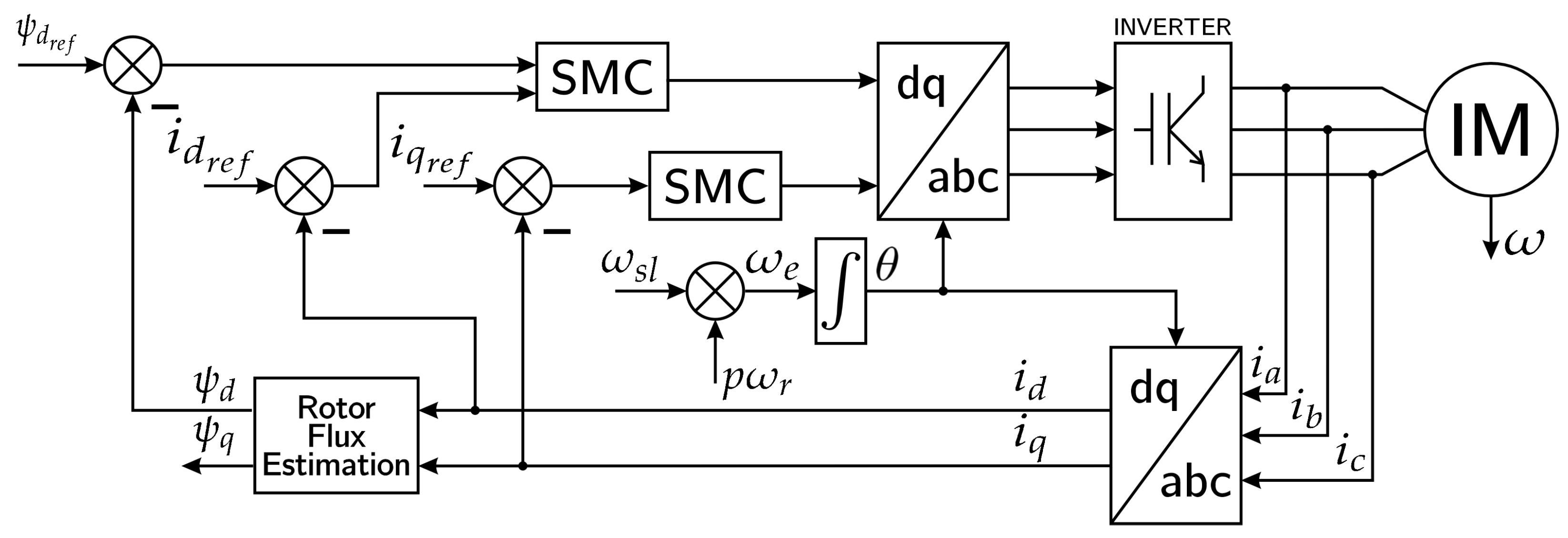
Block diagram of the considered control system is presented in Figure 1. For a better understanding of the problem, it should be pointed out that the rotor fluxes are not measurable and must be observed or estimated. In this paper we employ a half-virtual dynamics model of the IM that combine measured and estimated state variables. The elements of the actual flux vector ${\widehat{\psi }}_d={\widehat{\psi }}_d\left(t\right)$ and ${\widehat{\psi }}_q={\widehat{\psi }}_q\left(t\right)$ impact the IM currents. However, they cannot be included directly in the control law. Their estimates ${\psi }_d={\psi }_d\left(t\right)$ and ${\psi }_q={\psi }_q\left(t\right)$ are used instead. Alternatively put, within this framework, the element ${\widehat{\psi }}_d$ should be viewed as ${\psi }_d$ subject to some unknown perturbations.

Following this reasoning, we adopt the following machine description in the dq-frame rotating with synchronous speed ${\omega }_e$ [36].

$$\begin{array}{cc}\hfill {\displaystyle \frac{d}{dt}}{i}_d& =-{\displaystyle \frac{R_s+R_r\frac{L_m^2}{L_r^2}}{L_{\sigma }}}{i}_d+{\omega }_e{i}_q+{\displaystyle \frac{R_r{L}_m}{L_{\sigma }{L}_r^2}}{\widehat{\psi }}_d+{\displaystyle \frac{L_{m}p{\omega }_r}{L_{\sigma }{L}_r}}{\widehat{\psi }}_q+{\displaystyle \frac{1}{L_{\sigma }}}{u}_d\hfill \\ \hfill {\displaystyle \frac{d}{dt}}{i}_q& =-{\omega }_e{i}_d-{\displaystyle \frac{R_s+R_r\frac{L_m^2}{L_r^2}}{L_{\sigma }}}{i}_q-{\displaystyle \frac{L_{m}p{\omega }_r}{L_{\sigma }{L}_r}}{\widehat{\psi }}_d+{\displaystyle \frac{R_r{L}_m}{L_{\sigma }{L}_r^2}}{\widehat{\psi }}_q+{\displaystyle \frac{1}{L_{\sigma }}}{u}_q\hfill \\ \hfill {\displaystyle \frac{d}{dt}}{\psi }_d& ={\displaystyle \frac{R_r}{L_r}}{L}_m{i}_d-{\displaystyle \frac{R_r}{L_r}}{\psi }_d+{\omega }_{sl}{\psi }_q\hfill \\ \hfill {\displaystyle \frac{d}{dt}}{\psi }_q& ={\displaystyle \frac{R_r}{L_r}}{L}_m{i}_q-{\omega }_{sl}{\psi }_d-{\displaystyle \frac{R_r}{L_r}}{\psi }_q\hfill \\ \hfill {\tau }_e& =p({\widehat{\psi }}_d{i}_q-{\widehat{\psi }}_q{i}_d)\hfill \end{array}$$

(1)

Symbols used in the above equations are explained in

Table 1. Definitions of symbols used in model description.

$u_d$, $u_q$	stator voltages in d, q axes, respectively	V
$i_d$, $i_q$	stator currents in d, q axes, respectively	A
${\widehat{\psi }}_d$, ${\widehat{\psi }}_q$	d and q coordinate of rotor flux vector	Wb
${\psi }_d$, ${\psi }_q$	d and q coordinate of rotor flux estimate vector	Wb
$R_s$, $R_r$	stator and rotor resistance	$\mathrm{\Omega }$
$L_s$, $L_r$	stator and rotor inductance	H
$L_m$	magnetizing inductance	H
$L_{\sigma }$	leakage inductance coefficient $L_{\sigma }={\displaystyle \frac{L_r{L}_s-L_m^2}{L_r}}$	H
${\omega }_e$	electrical synchronous speed	${\displaystyle \frac{\mathrm{rad}}{\mathrm{s}}}$
${\omega }_r$	mechanical angular speed of the motor	${\displaystyle \frac{\mathrm{rad}}{\mathrm{s}}}$
p	number of pole pairs	-
${\omega }_{sl}$	slip frequency ${\omega }_{sl}={\omega }_e-p{\omega }_r$	${\displaystyle \frac{\mathrm{rad}}{\mathrm{s}}}$
${\tau }_e$	normalized torque	Nm

. All the signals are represented with scalar values. Motor parameters $R_s$, $R_r$, $L_s$, $L_r$, $L_m$, $L_{\sigma }$, and p are considered time-invariant. Their values are known with limited but specified accuracy. Signals describing motor state are continuous-time and are represented by $i_d=i_d\left(t\right)$, $i_q=i_q\left(t\right)$, ${\psi }_d={\psi }_d\left(t\right)$, ${\psi }_q={\psi }_q\left(t\right)$, ${\omega }_e={\omega }_e\left(t\right)$, ${\omega }_r={\omega }_r\left(t\right)$, ${\omega }_{sl}={\omega }_{sl}\left(t\right)$, ${\tau }_e={\tau }_e\left(t\right)$.

Note that there exist two types of dq-frame transformation—amplitude-invariant and power-invariant. The former is adopted in this study. Whereas the dynamical equations presented in (1) are identical regardless of the chosen transformation type, the torque formula is not. Therefore, a normalized torque ${\tau }_e$ without transformation-dependent scaling factor is used in the model. It is dependent only on d- and q-axis currents and fluxes and the number of pole pairs p. This implies that the value of ${\tau }_e$ is proportional to the electromagnetic torque of the machine.

Rotor flux FOC is used in this study and hence, we define the slip frequency as

$${\omega }_{sl}={\displaystyle \frac{R_r}{L_r}}{\displaystyle \frac{L_m{i}_q}{{\psi }_d}}.$$

(2)

This relation is used to determine the electrical speed ${\omega }_e$ of the motor according to the relation stated in Table 1. One may easily verify that by substituting (2) to the q-axis flux equation from (1), the following is obtained

$${\displaystyle \frac{d}{dt}}{\psi }_q=-{\displaystyle \frac{R_r}{L_r}}{\psi }_q.$$

(3)

This equation leads to a conclusion that for the chosen dq-frame synchronization method, the value of ${\psi }_q$ tends to zero regardless of the initial condition. This also simplifies the dynamics of ${\psi }_d$, which is now given by

$${\displaystyle \frac{d}{dt}}{\psi }_d=-{\displaystyle \frac{R_r}{L_r}}{\psi }_d+{\displaystyle \frac{R_r}{L_r}}{L}_m{i}_d+{\delta }_{{\psi }_d},$$

(4)

where ${\delta }_{{\psi }_d}$ is an exponentially decaying signal representing the solution of (3). Also, considering the steady state, the employed definition of ${\omega }_{sl}$ leads to a proportional relation of the stator current and the rotor flux, namely ${\psi }_d=L_m{i}_d$.

Nonetheless, small deviations of ${\psi }_q$ from zero caused by temporary loss of dq-frame synchronization are possible, and happen sometimes in practical case. Due to this fact, the estimated value of ${\psi }_q$ should be included in the control laws. Moreover, the slip definition given in (2) is highly dependent on the motor parameter identification accuracy. This may impact the dq-frame orientation causing larger differences between flux vector elements ${\widehat{\psi }}_d$, ${\widehat{\psi }}_q$ and their estimates ${\psi }_d$, ${\psi }_q$.

As the employed IM model is now explained, let us consider a decoupling feed-forward control for d- and q-axis currents. It was already mentioned that the motor parameters are not known exactly. Therefore, redefinition of the control signals introduces perturbations ${\delta }_{i_d}$ and ${\delta }_{i_q}$. They represent the aggregate differences between the real system and its mathematical model, arising from parameter identification and flux estimation error. Introducing virtual control voltages $v_d$ and $v_q$, defining control signals as

$$\begin{array}{c}{u}_d=v_d-L_{\sigma }{\omega }_e{i}_q-{\displaystyle \frac{L_{m}p{\omega }_r}{L_r}}{\psi }_q+{\delta }_{i_d}\hfill \\ u_q=v_q+L_{\sigma }{\omega }_e{i}_d+{\displaystyle \frac{L_{m}p{\omega }_r}{L_r}}{\psi }_d+{\delta }_{i_q}\hfill \end{array}$$

(5)

and substituting them into (1), one obtains two independent perturbed dynamical systems for d-axis

$$\begin{array}{cc}\hfill {\displaystyle \frac{d}{dt}}{i}_d& =-{\displaystyle \frac{R_s+R_r\frac{L_m^2}{L_r^2}}{L_{\sigma }}}{i}_d+{\displaystyle \frac{R_r{L}_m}{L_{\sigma }{L}_r^2}}{\psi }_d+{\displaystyle \frac{1}{L_{\sigma }}}{v}_d+{\delta }_{i_d}\hfill \\ \hfill {\displaystyle \frac{d}{dt}}{\psi }_d& =-{\displaystyle \frac{R_r}{L_r}}{\psi }_d+{\displaystyle \frac{R_r}{L_r}}{L}_m{i}_d+{\delta }_{{\psi }_d}\hfill \end{array}$$

(6)

and for q-axis state variables

$$\begin{array}{cc}\hfill {\displaystyle \frac{d}{dt}}{i}_q& =-{\displaystyle \frac{R_s+R_r\frac{L_m^2}{L_r^2}}{L_{\sigma }}}{i}_q+{\displaystyle \frac{R_r{L}_m}{L_{\sigma }{L}_r^2}}{\psi }_q+{\displaystyle \frac{1}{L_{\sigma }}}{v}_q+{\delta }_{i_q}\hfill \\ \hfill {\displaystyle \frac{d}{dt}}{\psi }_q& =-{\displaystyle \frac{R_r}{L_r}}{\psi }_q.\hfill \end{array}$$

(7)

The system dynamics in both axes are, therefore, decoupled. The virtual controls $v_d$ and $v_q$ will be developed later in the paper.

The introduced perturbations ${\delta }_{i_d}$, ${\delta }_{i_q}$, as well as the exponentially decaying signal ${\delta }_{{\psi }_d}$, are assumed to be bounded by positive constants ${\Delta }_{i_d},{\Delta }_{i_q},{\Delta }_{{\psi }_d}$ with respect to the absolute values, namely

$$\begin{array}{ccc}|{\delta }_{i_d}|<{\Delta }_{i_d},& |{\delta }_{i_q}|<{\Delta }_{i_q},& |{\delta }_{{\psi }_d}|<{\Delta }_{{\psi }_d}.\end{array}$$

(8)

This assumption does not impact the generality of the presented solution, as all signals are limited in practical implementations, and the bounds are arbitrary.

Having considered the above information, we now proceed to the main focus of this paper. To increase the performance of a drive system, it is important to develop fast torque control. In multi-level or cascade motor control systems, torque controller is the one acting closest to the motor. Hence, the performance of speed or position control highly depends on it.

The electromagnetic torque is always proportional to the signal ${\tau }_e$ defined in (1). Due to the selected dq-frame synchronization rule, this value is approximately equal to the product of ${\psi }_d$ and $i_q$ multiplied by p. Therefore, the dynamics of the motor torque depends mostly on these two state variables.

In this study we propose a sliding mode torque control approach to deliver a method allowing to decrease torque time constant. Separate controllers are defined for d- and q-axis. In case of the q-axis control, the main focus is put on reaching the reference $i_q$ current value in the shortest time possible. For the d-axis, a particular sliding manifold is defined, and it is shown how its definition impacts the motor torque time constant.

In the following sections of the paper, we present the subsequent elements of the control system in the following order. Firstly, a time-varying SMC algorithm for q-axis current presented in [25] is employed to obtain fast q-axis current control. Then, we propose a sliding manifold definition for d-axis flux control. The characteristics of this SMC are considered to give a better understanding of the whole control system.

3. Q-Axis Sliding Mode Controller

Since the dq-frame is oriented with respect to the definition of slip frequency ${\omega }_{sl}$, the value of q-axis flux ${\psi }_q=0$ with exception to particular scenarios, when the synchronization is temporarily lost. Hence, it is not necessary and would be negatively redundant to control ${\psi }_q$, and only a current controller should be used for the q-axis. This statement is additionally supported by the fact that when (2) is true, the state variable ${\psi }_q$ is not controllable via any of the control signals, which is visible in (7).

We define the q-axis sliding variable as

$$s_q=s_q\left(t\right)=\left\{\begin{array}{cc}{e}_{i_q}+a+bt\hfill & t<t_0\hfill \\ e_{i_q}\hfill & t\ge t_0\hfill \end{array}\right.,$$

(9)

where $e_q=i_{q_{ref}}-i_q$ and a, b, $t_0$ are constants. The sliding manifold is defined by putting $s_q=0$. This is a first-order system. This implies that the convergence of $s_q$ to zero is equivalent with reaching zero value of the control error $e_q$. Additionally, the employed sliding variable definition is time-varying and follows a linearly changing function $f\left(t\right)=a+bt$. For properly chosen parameters a and b, such definition eliminates the reaching phase and grants robustness of the system from the beginning of the control process [14].

For the control law we take

$$v_q=L_{\sigma }{\displaystyle \frac{d}{dt}}{i}_{q_{ref}}+\left(R_s+R_r{\displaystyle \frac{L_m^2}{L_r^2}}\right)i_q-{\displaystyle \frac{R_r{L}_m}{L_r^2}}{\psi }_q+L_{\sigma }{\gamma }_q\mathrm{sgn}\left(s_q\right)+\left\{\begin{array}{cc}{L}_{\sigma }b\hfill & t<t_0\hfill \\ 0\hfill & t\ge t_0\hfill \end{array}\right.,$$

(10)

with constant ${\gamma }_q>0$.

To verify the stability of the sliding mode under such control, let us analyze the Lyapunov function

$$V\left(s_q\right)={\displaystyle \frac{1}{2}}{s}_q^2.$$

(11)

Calculating its derivative and substituting (7) and (10) we obtain

$${\displaystyle \frac{d}{dt}}V\left(s_q\right)=-{\gamma }_q{s}_q\mathrm{sgn}\left(s_q\right)-s_q{\delta }_{i_q}$$

(12)

for both time intervals $t<t_0$ and $t\ge t_0$. Since the value of ${\delta }_{i_q}$ is bounded as in (8), we write

$${\displaystyle \frac{d}{dt}}V\left(s_q\right)\le -{\gamma }_q|s_q|+|s_q{\delta }_{i_q}|<|s_q|({\Delta }_{i_q}-{\gamma }_q).$$

(13)

Hence, the stability of the considered sliding mode is guaranteed for ${\gamma }_q>{\Delta }_{i_q}$. Based on this knowledge, the value of ${\gamma }_q$ depends on the accuracy of the motor parameter identification and must be chosen separately for each application. For instance, parameter ${\gamma }_q$ may be chosen by performing an experimental motor run as a maximum value of the difference between the applied voltage and the equivalent voltage calculated with Formula (10) for ${\gamma }_q=0$ and $b=0$.

As stated in [14], we chose the control parameters a and b as

$$a=-e_{i_q}\left(0\right),b={\displaystyle \frac{e_{i_q}\left(0\right)}{t_0}},$$

(14)

where $t_0$ is the time in which the current error reaches zero. This way, the reaching phase is eliminated and the sliding motion is occurring during the whole control process. Time $t_0$ may be chosen arbitrary, bearing in mind that decreasing it requires higher voltage limit as parameter b is present directly in the control law (10). Moreover, the stability at the moment when the sliding variable reaches zero is also guaranteed, and the argument for that can be found in [14].

If the parameters are chosen as stated above and the supply voltage limit is sufficient, the system representative point remains on the sliding manifold for all time $t\ge 0$, and hence we may write

$$e_q=\left\{\begin{array}{ccc}\left(1-{\displaystyle \frac{t}{t_0}}\right)e_{i_q}\left(0\right)& \mathrm{for}\hfill & t<t_0\hfill \\ 0& \mathrm{for}\hfill & t\ge t_0\hfill \end{array}\right..$$

(15)

Therefore we know that the desired q-axis current value is reached in prescribed time $t_0$. Although this time is arbitrary, it should be, and usually is, significantly lower then the flux time constant. Hence, the torque control performance is mostly dependent on the rotor flux behavior. The next section considers d-axis flux control that aims at increasing the rotor flux convergence rate.

4. D-Axis Sliding Mode Controller

We consider the second order linear perturbed system given by (6) that describes d-axis current and flux dynamics under the considered conditions. We define the d-axis sliding variable as

$$s_d=e_{i_d}+\beta e_{{\psi }_d}$$

(16)

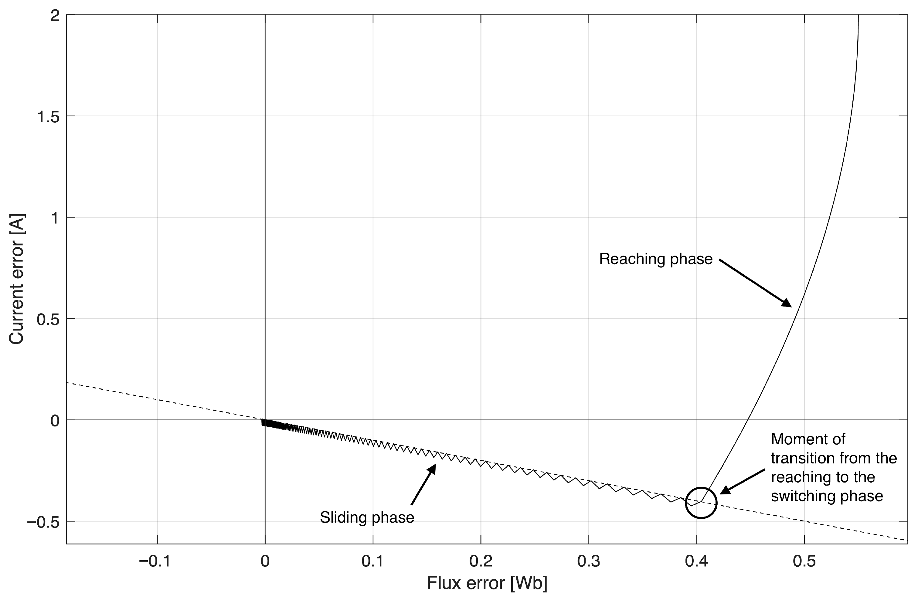
where $\beta >0$ is a constant, $e_{i_d}=i_{d_{ref}}-i_d$ is d-axis current control error, and $e_{{\psi }_d}={\psi }_{d_{ref}}-{\psi }_d$ is d-axis flux control error. We define the sliding manifold by putting $s_d=0$. An example of practical sliding mode trajectory for the considered system is presented in Figure 2.

The control law stabilizing the system is given by

$$\begin{array}{cc}\hfill v_d& =L_{\sigma }{\displaystyle \frac{d}{dt}}{i}_{d_{ref}}+\left(R_s+R_r{\displaystyle \frac{L_m^2}{L_r^2}}\right)i_d-{\displaystyle \frac{R_r{L}_m}{L_r^2}}{\psi }_d+\hfill \\ \hfill & +\beta L_{\sigma }{\displaystyle \frac{d}{dt}}{\psi }_{d_{ref}}+\beta L_{\sigma }{\displaystyle \frac{R_r}{L_r}}{\psi }_d-\beta L_{\sigma }{\displaystyle \frac{R_r}{L_r}}{L}_m{i}_d+L_{\sigma }{\gamma }_d\mathrm{sgn}\left(s_d\right)\hfill \end{array}.$$

(17)

The stability of the sliding mode can be proved by analyzing the Lyapunov function

$$V\left(s_d\right)={\displaystyle \frac{1}{2}}{s}_d^2.$$

(18)

Its derivative is equal to

$$\begin{array}{cc}\hfill {\displaystyle \frac{d}{dt}}V\left(s_d\right)=s_d(& {\displaystyle \frac{d}{dt}}{i}_{d_{ref}}+{\displaystyle \frac{R_s+R_r\frac{L_m^2}{L_r^2}}{L_{\sigma }}}{i}_d-{\displaystyle \frac{R_r{L}_m}{L_{\sigma }{L}_r^2}}{\psi }_d-{\displaystyle \frac{1}{L_{\sigma }}}{v}_d+\hfill \\ \hfill & +\beta {\displaystyle \frac{d}{dt}}{\psi }_{d_{ref}}+\beta {\displaystyle \frac{R_r}{L_r}}{\psi }_d-\beta {\displaystyle \frac{R_r}{L_r}}{L}_m{i}_d-{\delta }_{i_d}-\beta {\delta }_{{\psi }_d})\hfill \end{array}.$$

(19)

Substituting the control signal (17) we get

$${\displaystyle \frac{d}{dt}}V\left(s_d\right)=-{\gamma }_d{s}_d\mathrm{sgn}\left(s_d\right)-s_d({\delta }_{i_d}+\beta {\delta }_{{\psi }_d})$$

(20)

and, since ${\delta }_{i_d}$ and ${\delta }_{{\psi }_d}$ are bounded, we may write

$${\displaystyle \frac{d}{dt}}V\left(s_d\right)\le -{\gamma }_d|s_d|+|s_d|\left|{\delta }_{i_d}+\beta {\delta }_{{\psi }_d}\right|<\left|s_d\right|\left({\Delta }_{i_d}+\beta {\delta }_{{\psi }_d}-{\gamma }_d\right).$$

(21)

Introducing ${\Delta }_d={\Delta }_{i_d}+\beta {\delta }_{{\psi }_d}$, we may write

$${\displaystyle \frac{d}{dt}}V\left(s_d\right)<\left|s_d\right|\left({\Delta }_d-{\gamma }_d\right).$$

(22)

Therefore, the sliding mode is globally asymptotically stable for ${\gamma }_d>{\Delta }_d$.

As mentioned before, d-axis current and d-axis flux remain in a proportional relation in the steady state due to the chosen definition of ${\omega }_{sl}$. Therefore, regarding the reference current and flux values, the following equation must be satisfied

$${\psi }_{d_{ref}}=L_m{i}_{d_{ref}}.$$

(23)

The properties of the system (6) under control law (17) are analyzed in the two subsections below.

4.1. Reaching Phase Behavior

Firstly, let us analyze the reaching phase behavior. In general, three scenarios are possible when the control process commences—the sliding variable can be either positive, negative or equal to zero. In the third case, the reaching phase is eliminated, which is why it will not be considered in this paragraph. For the remaining two scenarios, the difference is subtle, and one can easily switch between them.

Consider a situation when $s_d\left(0\right)>0$. Using Equation (6), assuming $i_{d_{ref}}=\mathrm{const}$ and substituting (17), we may express the system dynamics under the proposed sliding mode control in the matrix form as

$${\displaystyle \frac{d}{dt}}{\mathbf{x}}_{\mathbf{d}}=\left[\begin{array}{cc}-\beta {\displaystyle \frac{R_r}{L_r}}{L}_m& \beta {\displaystyle \frac{R_r}{L_r}}\\ {\displaystyle \frac{R_r}{L_r}}{L}_m& -{\displaystyle \frac{R_r}{L_r}}\end{array}\right]{\mathbf{x}}_{\mathbf{d}}+\left[\begin{array}{c}{\gamma }_d\\ 0\end{array}\right]+\left[\begin{array}{c}{\delta }_{i_d}\\ {\delta }_{{\psi }_d}\end{array}\right],$$

(24)

where ${\mathbf{x}}_{\mathbf{d}}={\left[i_d{\psi }_d\right]}^T$. One may notice that this system is linear. Hence, the superposition rule holds. Let us analyze the response of the system excluding the perturbances ${\delta }_{i_d}$ and ${\delta }_{{\psi }_d}$ with initial condition ${\mathbf{x}}_{{\mathbf{d}}_{\mathbf{0}}}={\left[i_{d_0}{\psi }_{d_0}\right]}^T$.

The transition matrix of the system is equal to

$$\mathbf{\Phi }\left(t\right)={\displaystyle \frac{1}{1+\beta L_m}}\left[\begin{array}{cc}1+\beta L_m{e}^{-{\displaystyle \frac{R_r}{L_r}}(1+\beta L_m)t}& \beta -\beta e^{-{\displaystyle \frac{R_r}{L_r}}(1+\beta L_m)t}\\ L_m-L_m{e}^{-{\displaystyle \frac{R_r}{L_r}}(1+\beta L_m)t}& \beta L_m+e^{-{\displaystyle \frac{R_r}{L_r}}(1+\beta L_m)t}\end{array}\right].$$

(25)

Using the formula

$${\mathbf{x}}_{\mathbf{d}}\left(t\right)=\mathbf{\Phi }\left(t\right){\mathbf{x}}_{{\mathbf{d}}_{\mathbf{0}}}+{\int }_0^t\mathbf{\Phi }(t-\tau )\left[\begin{array}{c}{\gamma }_d\\ 0\end{array}\right]d\tau$$

(26)

we get

$${\mathbf{x}}_{\mathbf{d}}\left(t\right)=\mathbf{\Phi }\left(t\right){\mathbf{x}}_{{\mathbf{d}}_{\mathbf{0}}}+{\displaystyle \frac{{\gamma }_d}{1+\beta L_m}}\left[\begin{array}{cc}1& {\displaystyle \frac{\beta L_m{L}_r}{R_r(1+\beta L_m)}}\\ L_m& -{\displaystyle \frac{L_m{L}_r}{R_r(1+\beta L_m)}}\end{array}\right]\left[\begin{array}{c}t\\ 1-e^{-{\displaystyle \frac{R_r}{L_r}}(1+\beta L_m)t}\end{array}\right].$$

(27)

Dividing this matrix state equation into two separate scalar equations, the current and the flux signals are obtained as

$$\begin{array}{cc}\hfill i_d\left(t\right)={\displaystyle \frac{1}{1+\beta L_m}}\left[\left(1+\beta L_m{e}^{-{\displaystyle \frac{R_r}{L_r}}(1+\beta L_m)t}\right)\right.i_{d_0}& +\beta \left(1-e^{-{\displaystyle \frac{R_r}{L_r}}(1+\beta L_m)t}\right){\psi }_{d_0}+{\gamma }_{d}t+\hfill \\ \hfill & +\left.{\displaystyle \frac{{\gamma }_d\beta L_m{L}_r}{R_r(1+\beta L_m)}}\left(1-e^{-{\displaystyle \frac{R_r}{L_r}}(1+\beta L_m)t}\right)\right]\hfill \end{array}$$

(28)

and

$$\begin{array}{cc}\hfill {\psi }_d\left(t\right)={\displaystyle \frac{1}{1+\beta L_m}}\left[\left(\beta L_m+e^{-{\displaystyle \frac{R_r}{L_r}}(1+\beta L_m)t}\right){\psi }_{d_0}\right.& +L_m\left(1-e^{-{\displaystyle \frac{R_r}{L_r}}(1+\beta L_m)t}\right)i_{d_0}+L_m{\gamma }_{d}t+\hfill \\ \hfill & -\left.{\displaystyle \frac{{\gamma }_d{L}_m{L}_r}{R_r(1+\beta L_m)}}\left(1-e^{-{\displaystyle \frac{R_r}{L_r}}(1+\beta L_m)t}\right)\right].\hfill \end{array}$$

(29)

As for the other case, when $s_d\left(0\right)<0$, it can be considered analogously by changing the sign before the vector containing ${\gamma }_d$ in (24). After analyzing the equations, one may see that it implies the analogous change of sign before the elements containing ${\gamma }_d$ in (28) and (29). This change does not affect the transition matrix, which is a convenient property.

If the reaching phase duration time is equal to $t_r$, then ${\forall }_{t\ge t_r}{s}_d\left(t\right)=0$. At $t_r$, the sliding manifold is crossed by the system trajectory for the first time. This is also the last moment, when Equations (24) and (27)–(29) apply. Bearing (23) in mind, we may substitute $i_{d_{ref}}$, $i_d$, ${\psi }_{d_{ref}}$ and ${\psi }_d$ into (16) to calculate the theoretical value of $t_r$. Doing so, we obtain

$$\begin{array}{cc}\hfill s_d\left(t_r\right)& =i_{d_{ref}}+\beta {\psi }_{d_{ref}}-{\displaystyle \frac{1}{1+\beta L_m}}\left[\left(1+\beta L_m{e}^{-{\displaystyle \frac{R_r}{L_r}}(1+\beta L_m)t_r}\right)\right.i_{d_0}+\beta \left(1-e^{-{\displaystyle \frac{R_r}{L_r}}(1+\beta L_m)t_r}\right){\psi }_{d_0}+\hfill \\ \hfill & +{\displaystyle \frac{\beta L_m{L}_r}{R_r(1+\beta L_m)}}\left(1-e^{-{\displaystyle \frac{R_r}{L_r}}(1+\beta L_m)t_r}\right)-{\displaystyle \frac{L_m{L}_r}{R_r(1+\beta L_m)}}\left(1-e^{-{\displaystyle \frac{R_r}{L_r}}(1+\beta L_m)t_r}\right)+\hfill \\ \hfill & -\beta \left(\beta L_m+e^{-{\displaystyle \frac{R_r}{L_r}}(1+\beta L_m)t_r}\right){\psi }_{d_0}+\left.\beta L_m\left(1-e^{-{\displaystyle \frac{R_r}{L_r}}(1+\beta L_m)t_r}\right)i_{d_0}+\beta L_m{\gamma }_d{t}_r+{\gamma }_d{t}_r\right]=0.\hfill \end{array}$$

(30)

Rearranging the equation and solving for $t_r$, one finally gets

$$t_r={\displaystyle \frac{1}{{\gamma }_d}}\left[(1+\beta L_m)i_{d_{ref}}-\beta {\psi }_{d_0}-i_{d_0}\right].$$

(31)

This formula is true for $s_d\left(0\right)>0$. If $s_d\left(0\right)<0$, the sign of the right-hand side of the equation above must be reversed due to the change of sign of the expression in square brackets. This fact can be checked by assuming $s_d\left(0\right)<0$ and repeating the steps presented in this section.

The conclusion from the presented analysis is that one may impact the reaching time of the sliding mode by changing the parameters ${\gamma }_d$ and $\beta$. Increasing ${\gamma }_d$ shortens the duration of the reaching phase, and increasing $\beta$ extends it. It is important that none of the elements may be infinitely increased or equal to zero.

Assuming that the rotor flux is not forced to change sign during the motor restart, i.e., ${\psi }_{d_{ref}}{\psi }_{d_0}>0$, the maximal duration of the reaching phase can be calculated from Equation (31) by putting ${\psi }_{d_0}=0$ and $i_{d_0}=0$ and is equal to

$$t_{r,max}={\displaystyle \frac{1}{{\gamma }_d}}\left(1+\beta L_m\right)\left|i_{d_{ref}}\right|.$$

(32)

The absolute value generalizes the equation for both $s_d\left(0\right)>0$ and $s_d\left(0\right)<0$.

The assumption that the rotor flux does not change sign does not necessarily impact the generality of the analysis in the considered scenario. The electromagnetic torque of the IM is proportional to the product of d-axis rotor flux and q-axis stator current. Hence, the sign of the torque can be modified by changing the sign of the desired value of q-axis current $i_{q_{ref}}$, while leaving the d-axis reference flux sign unchanged.

One should note that for $i_{d_0}=0$, the current $i_d$ is strictly monotonous during the reaching phase, which follows from (28). The maximal value of the d-axis current is obtained by substituting $t_r$ to this equation. In particular, for zero initial conditions and $i_{d_{ref}}>0$, the maximal value of $i_d$ current is given by

$$i_{d_{max}}=i_{d_{ref}}+{\displaystyle \frac{{\gamma }_d\beta L_m{L}_r}{R_r{(1+\beta L_m)}^2}}\left(1-e^{-{\displaystyle \frac{R_r}{{\gamma }_d{L}_r}}{(1+\beta L_m)}^2{i}_{d_{ref}}}\right).$$

(33)

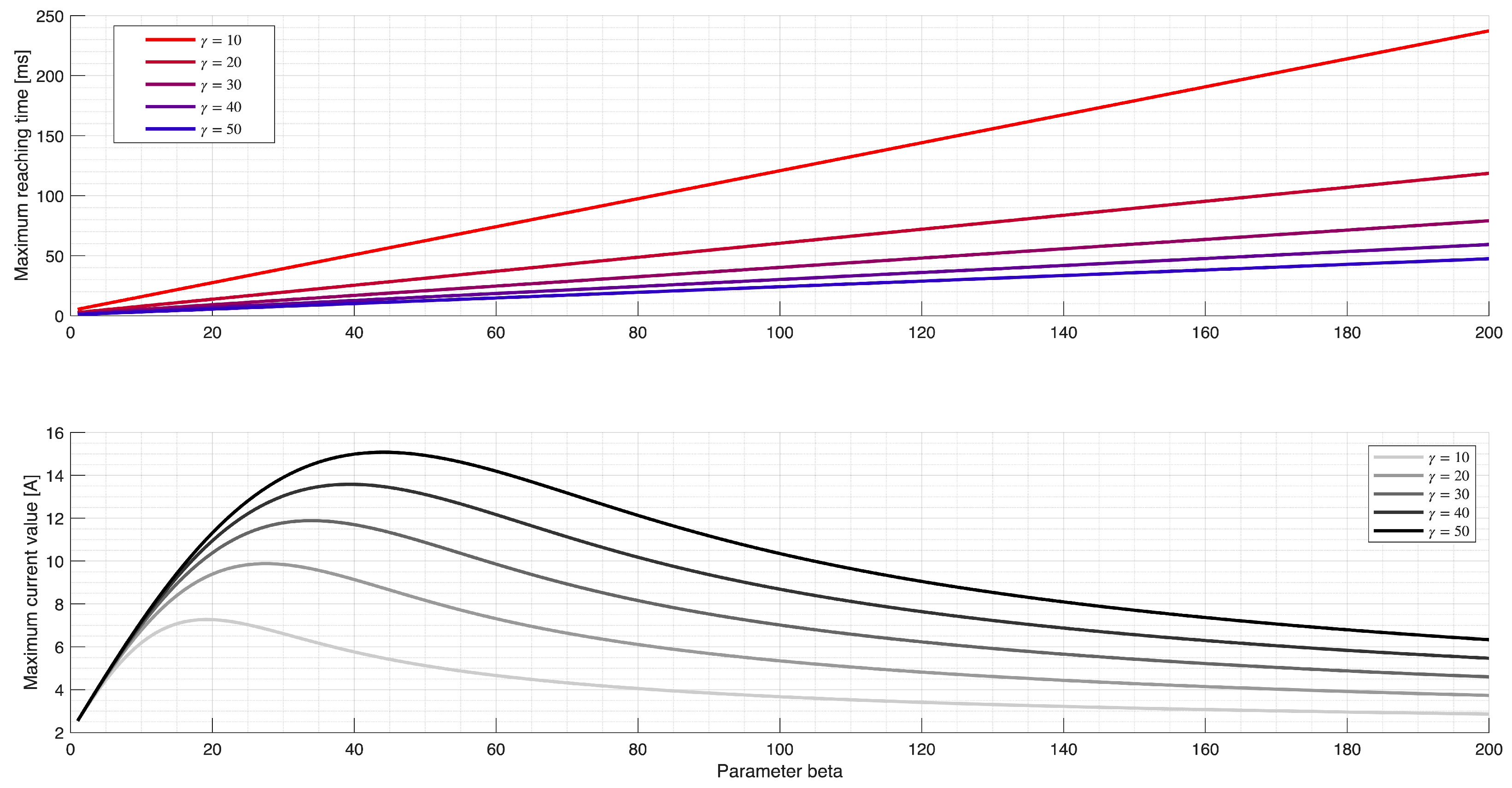
Another important observation that also follows from (28) is that for sufficiently large values of the $\beta /{\gamma }_d$ ratio, the free response vanishes rapidly enough for the current response to become linear. Because of this phenomenon, the maximum current value does not increase infinitely with $\beta$. To illustrate this, Equations (31) and (33) are presented graphically in Figure 3.

Figure 3. Predicted maximum reaching time and maximum d-axis current for motor parameters from the Table 2 and $i_{d_{ref}}=2$ A. The letter $\gamma$ in the legend represents the switching voltage amplitude, that is $\gamma =L_{\sigma }{\gamma }_d$.

Figure 3. Predicted maximum reaching time and maximum d-axis current for motor parameters from the Table 2 and $i_{d_{ref}}=2$ A. The letter $\gamma$ in the legend represents the switching voltage amplitude, that is $\gamma =L_{\sigma }{\gamma }_d$.

Table 2. Identified parameters of the induction machine used for the laboratory tests.

Parameter	Value	Description
$R_s$	2.84	stator winding resistance [$\mathrm{\Omega }$]
$R_r$	2.73	rotor winding resistance [$\mathrm{\Omega }$]
$L_s$	285.8	stator winding inductance [mH]
$L_r$	285.8	rotor winding inductance [mH]
$L_m$	275.0	magnetizing inductance [mH]
p	2	number of pole pairs [-]

Table 2. Identified parameters of the induction machine used for the laboratory tests.

Parameter	Value	Description
$R_s$	2.84	stator winding resistance [$\mathrm{\Omega }$]
$R_r$	2.73	rotor winding resistance [$\mathrm{\Omega }$]
$L_s$	285.8	stator winding inductance [mH]
$L_r$	285.8	rotor winding inductance [mH]
$L_m$	275.0	magnetizing inductance [mH]
p	2	number of pole pairs [-]

4.2. Sliding Phase Behavior

It has already been shown that the proposed sliding mode (16) is globally asymptotically stable for a properly chosen value of ${\gamma }_d$ and that the sliding manifold is reached in finite time, which was calculated in the previous section. Since the sliding motion is guaranteed, the next step is to consider the behavior of the system on the sliding manifold.

When the sliding motion happens, the sliding variable $s_d\left(t\right)=0$. Hence, the response of the system can be calculated using equation

$${\mathbf{x}}_{\mathbf{d}}\left(t\right)=\mathbf{\Phi }\left(t\right){\mathbf{x}}_{{\mathbf{d}}_{\mathbf{1}}},$$

(34)

where ${\mathbf{x}}_{{\mathbf{d}}_{\mathbf{1}}}={\left[i_{d_1}{\psi }_{d_1}\right]}^T={\mathbf{x}}_{\mathbf{d}}\left(t_r\right)$ is the system state at time $t_r$, when the sliding manifold is crossed for the first time. Calculating the current and the flux response, one obtains

$$i_d\left(t\right)={\displaystyle \frac{1}{1+\beta L_m}}\left[\left(1+\beta L_m{e}^{-{\displaystyle \frac{R_r}{L_r}}(1+\beta L_m)t}\right)i_{d_1}+\beta \left(1-e^{-{\displaystyle \frac{R_r}{L_r}}(1+\beta L_m)t}\right){\psi }_{d_1}\right],$$

(35)

$${\psi }_d\left(t\right)={\displaystyle \frac{1}{1+\beta L_m}}\left[\left(\beta L_m+e^{-{\displaystyle \frac{R_r}{L_r}}(1+\beta L_m)t}\right){\psi }_{d_1}+L_m\left(1-e^{-{\displaystyle \frac{R_r}{L_r}}(1+\beta L_m)t}\right)i_{d_1}\right].$$

(36)

Calculating the limit $i_{d_{\infty }}={lim}_{t\to \infty }{i}_d\left(t\right)$, we get

$$i_{d_{\infty }}={\displaystyle \frac{1}{1+\beta L_m}}\left(i_{d_1}+\beta {\psi }_{d_1}\right).$$

(37)

Since $s_d\left(t_r\right)=i_{d_{ref}}-i_{d_1}+\beta {\psi }_{d_{ref}}-\beta {\psi }_{d_1}=0$, using (23) we may write

$$i_{d_{ref}}(1+\beta L_m)=i_{d_1}+\beta {\psi }_{d_1}$$

(38)

and after substituting it to (37), we get

$$i_{d_{\infty }}=i_{d_{ref}}.$$

(39)

From the above equation and from (16) we conclude that

$${\psi }_{d_{\infty }}=\underset{t\to \infty }{lim}{\psi }_d\left(t\right)={\psi }_{d_{ref}}.$$

(40)

This shows that not only the sliding mode is globally asymptotically stable but also the state variables converge to their reference values. Moreover, using (38), we may simplify Equations (35) and (36) by rewriting them as

$$i_d\left(t\right)=i_{d_{ref}}+{\displaystyle \frac{\beta }{1+\beta L_m}}(L_m{i}_{d_1}-{\psi }_{d_1})e^{-{\displaystyle \frac{R_r}{L_r}}(1+\beta L_m)t}$$

(41)

and

$${\psi }_d\left(t\right)={\psi }_{d_{ref}}-{\displaystyle \frac{1}{1+\beta L_m}}(L_m{i}_{d_1}-{\psi }_{d_1})e^{-{\displaystyle \frac{R_r}{L_r}}(1+\beta L_m)t}.$$

(42)

The flux response equation above implies, that the largest flux time constant is obtained for $\beta =0$. Any value of this parameter admissible from the point of view of the presented strategy, i.e., any $\beta >0$, decreases it.

4.3. Perturbation Impact on System Behavior

Perturbations present in (24) were not considered so far. For ${\delta }_{i_d}\ne 0$, ${\delta }_{{\psi }_d}\ne 0$, the formula describing system state response changes to

$${\tilde{\mathbf{x}}}_{\mathbf{d}}={\mathbf{x}}_{\mathbf{d}}+{\int }_0^t\mathbf{\Phi }(t-\tau )\left[\begin{array}{c}{\delta }_{i_d}\\ {\delta }_{{\psi }_d}\end{array}\right]d\tau ,$$

(43)

where ${\mathbf{x}}_{\mathbf{d}}$ is given by (26). For convenience, we define

$$\delta {\mathbf{x}}_{\mathbf{d}}={\int }_0^t\mathbf{\Phi }(t-\tau )\left[\begin{array}{c}{\delta }_{i_d}\\ {\delta }_{{\psi }_d}\end{array}\right]d\tau .$$

(44)

The perturbations ${\delta }_{i_d}$ and ${\delta }_{{\psi }_d}$ are not known, and hence, $\delta {\mathbf{x}}_{\mathbf{d}}$ cannot be calculated. However, all of the elements of $\mathbf{\Phi }\left(t\right)$ given in (25) are non-negative and, therefore, we may write

$$\delta {\mathbf{x}}_{\mathbf{d}}⪯\Delta {\mathbf{x}}_{\mathbf{d}}={\int }_0^t\mathbf{\Phi }(t-\tau )\left[\begin{array}{c}{\Delta }_{i_d}\\ {\Delta }_{{\psi }_d}\end{array}\right]d\tau .$$

(45)

The symbol ⪯ denotes piecewise comparison of vectors. We know from (8) that inequality

$$-\Delta {\mathbf{x}}_{\mathbf{d}}⪯\delta {\mathbf{x}}_{\mathbf{d}}$$

(46)

is also always true.

Unlike in the ideal case, the exact reaching time cannot be calculated as the perturbations are not known. However, it is possible to find its lower and upper bound. Calculating the above integral, one obtains

$$\Delta {\mathbf{x}}_{\mathbf{d}}={\displaystyle \frac{1}{1+\beta L_m}}\left[\begin{array}{c}{\Delta }_{i_d}t+\beta {\Delta }_{{\psi }_d}t+{\displaystyle \frac{\beta L_r}{R_r(1+\beta L_m)}}\left(L_m{\Delta }_{i_d}-{\Delta }_{{\psi }_d}\right)\left(1-e^{-{\displaystyle \frac{R_r}{L_r}}(1+\beta L_m)t}\right)\\ L_m{\Delta }_{i_d}t+\beta L_m{\Delta }_{{\psi }_d}t-{\displaystyle \frac{L_r}{R_r(1+\beta L_m)}}\left(L_m{\Delta }_{i_d}-{\Delta }_{{\psi }_d}\right)\left(1-e^{-{\displaystyle \frac{R_r}{L_r}}(1+\beta L_m)t}\right)\end{array}\right].$$

(47)

Regarding the lower bound of $\delta {\mathbf{x}}_{\mathbf{d}}$ we write

$$\left[\begin{array}{cc}1& \beta \end{array}\right]\left[\begin{array}{c}{i}_{d_{ref}}\\ {\psi }_{d_{ref}}\end{array}\right]-\left[\begin{array}{cc}1& \beta \end{array}\right]{\tilde{\mathbf{x}}}_{\mathbf{d}}\le \left[\begin{array}{cc}1& \beta \end{array}\right]\left[\begin{array}{c}{i}_{d_{ref}}\\ {\psi }_{d_{ref}}\end{array}\right]-\left[\begin{array}{cc}1& \beta \end{array}\right]\left({\mathbf{x}}_{\mathbf{d}}-\Delta {\mathbf{x}}_{\mathbf{d}}\right),$$

(48)

which is always true for $\beta \ge 0$ if (45) applies. The left-hand side of this inequality is equal to the sliding variable ${\tilde{s}}_d$ defined as in (16) but with perturbed vector ${\tilde{\mathbf{x}}}_{\mathbf{d}}$ instead of the ideal one ${\mathbf{x}}_{\mathbf{d}}$. For such cases, we have ${\tilde{s}}_d\left({\tilde{t}}_r\right)=0$. Hence, considering the reaching time ${\tilde{t}}_r$ of the perturbed system, we may write

$$0\le s_d\left({\tilde{t}}_r\right)-\left[\begin{array}{cc}1& \beta \end{array}\right]\Delta {\mathbf{x}}_{\mathbf{d}}\left({\tilde{t}}_r\right).$$

(49)

Substituting (30) and (47), rearranging the equation and solving for ${\tilde{t}}_r$, one finally obtains

$${\tilde{t}}_r\le {\displaystyle \frac{1}{{\gamma }_d-{\Delta }_d}}\left[(1+\beta L_m)i_{d_{ref}}-\beta {\psi }_{d_0}-i_{d_0}\right].$$

(50)

A similar analysis can be performed for the upper bound of $\delta {\mathbf{x}}_{\mathbf{d}}$. In this alternative scenario, one gets

$${\tilde{t}}_r\ge {\displaystyle \frac{1}{{\gamma }_d+{\Delta }_d}}\left[(1+\beta L_m)i_{d_{ref}}-\beta {\psi }_{d_0}-i_{d_0}\right].$$

(51)

For the ideal case, the steady-state behavior was analyzed to show that the control error tends to zero. Equations (39) and (40) prove this statement. For the considered perturbed system, the matching conditions are not met by the perturbation ${\delta }_{{\psi }_d}$. Hence, one should also expect worse performance considering the steady state.

However, as discussed earlier, the signal ${\delta }_{{\psi }_d}$ is always decaying exponentially to zero. Any impact it may have on the system is temporary and the steady-state error is not affected. Therefore, the Equations (39) and (40) remain valid.

5. Experimental Results

This research is strongly oriented toward the practical application of sliding mode control. Parameters of the motor that is used for laboratory test have been identified beforehand and are listed in the Table 2.

Table 3. Nominal parameters of the induction machine.

Parameter	Value	Description
$n_n$	1420	nominal speed [rpm]
$P_n$	2200	nominal power [W]
$I_n$	4.85	nominal current [A]
$U_n$	400	nominal voltage [V]

presents the nominal motor voltage, current, power, and speed.

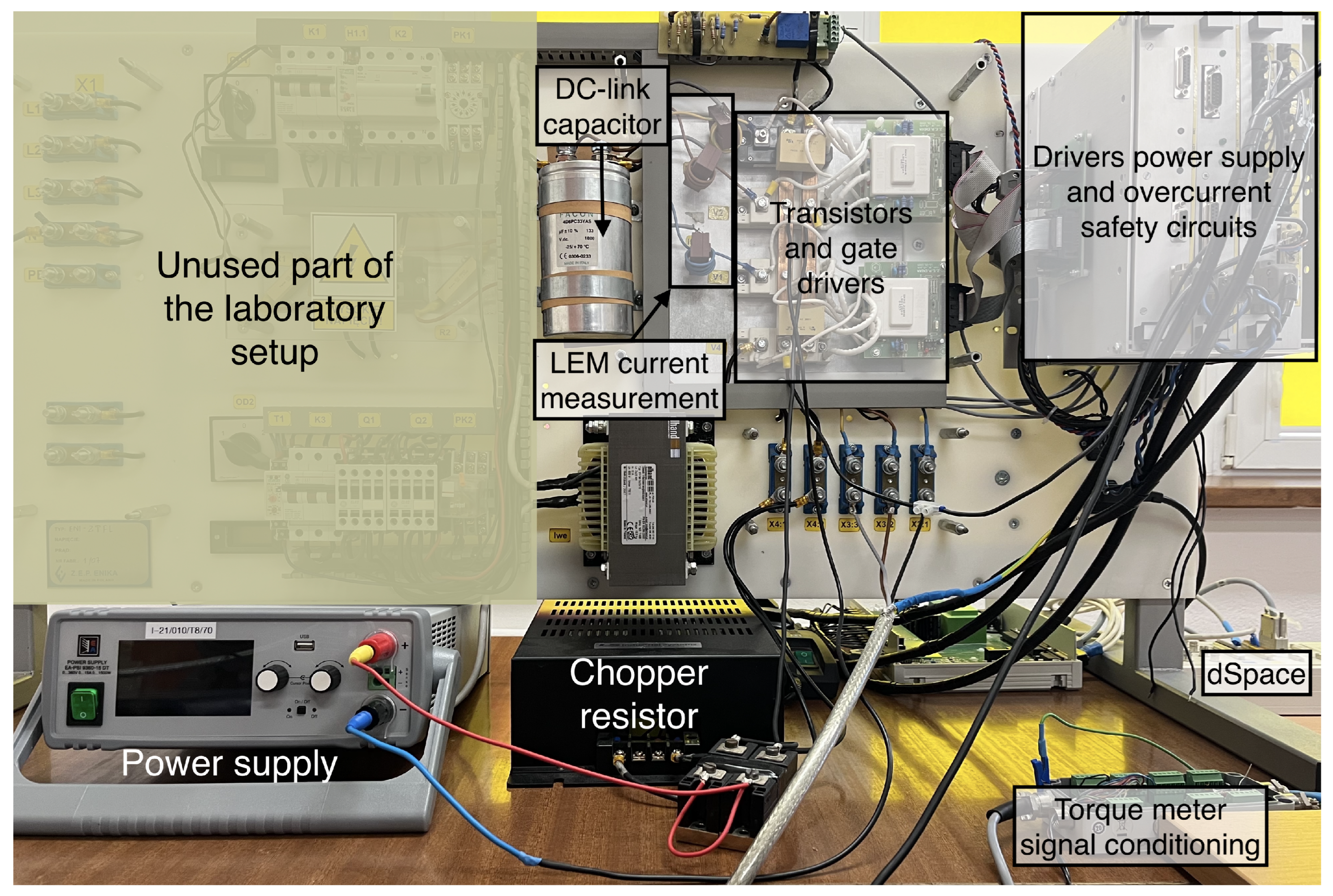
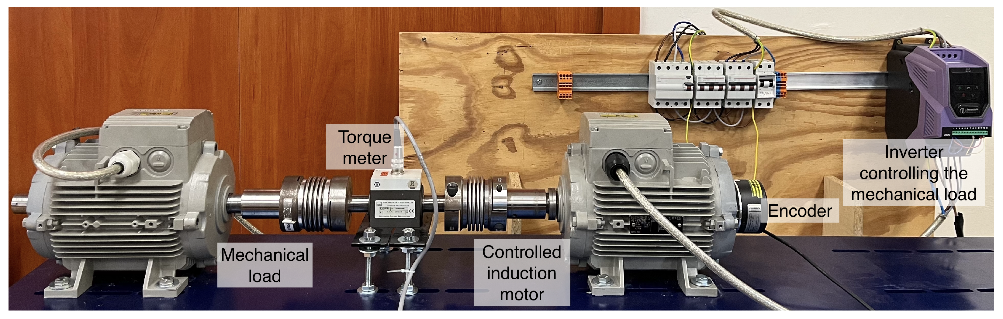
The laboratory stand consists of two identical induction motors. The first one is controlled by an industrial inverter using U/f = const control method. The task of this motor is to maintain a constant speed during the tests. The second one is the considered plant. It is supplied using an inverter controlled via dSpace hardware, which realizes the control algorithms created in MATLAB Simulink 2021b software. The full setup is presented in Figure 4 and Figure 5.

The prepared hardware measures all three of the phase currents, which are then used for dq-frame transformation. Motor speed is measured with incremental encoder. The DC-link voltage is also measured, and a chopper is used to dissipate the excess power and prevent the overvoltage from occurring. Torque meter is also used but only for verification and not for control.

Two main tests have been performed:

• motor startup for $\beta =10$ and different values of ${\omega }_r$ and
• motor startup for different values of $\beta$ and arbitrary chosen ${\omega }_r=47.6{\displaystyle \frac{\mathrm{rad}}{\mathrm{s}}}$.

The reference values for the d- and q-axis currents remain the same for all the tests and are equal $i_{d_{ref}}=2\mathrm{A}$, $i_{q_{ref}}=4.2\mathrm{A}$. The reference value of the d-axis flux follows from (23) and the value of parameter $L_m$ given in the Table 2. The switching voltage amplitudes are set to $20\mathrm{V}$, which means, that ${\gamma }_d={\gamma }_q={\displaystyle \frac{20}{L_{\sigma }}}$. 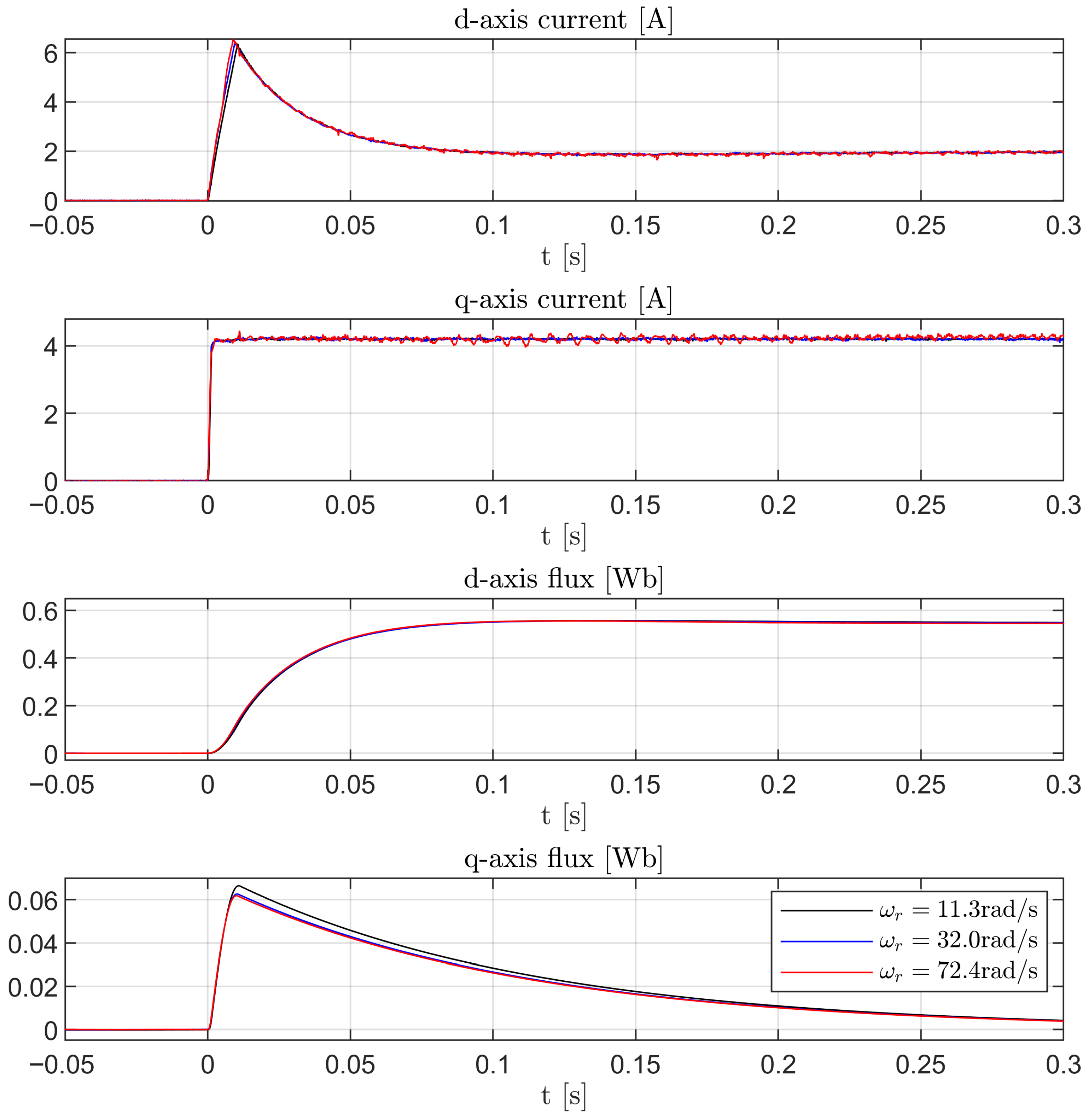These values are also invariant during the tests. 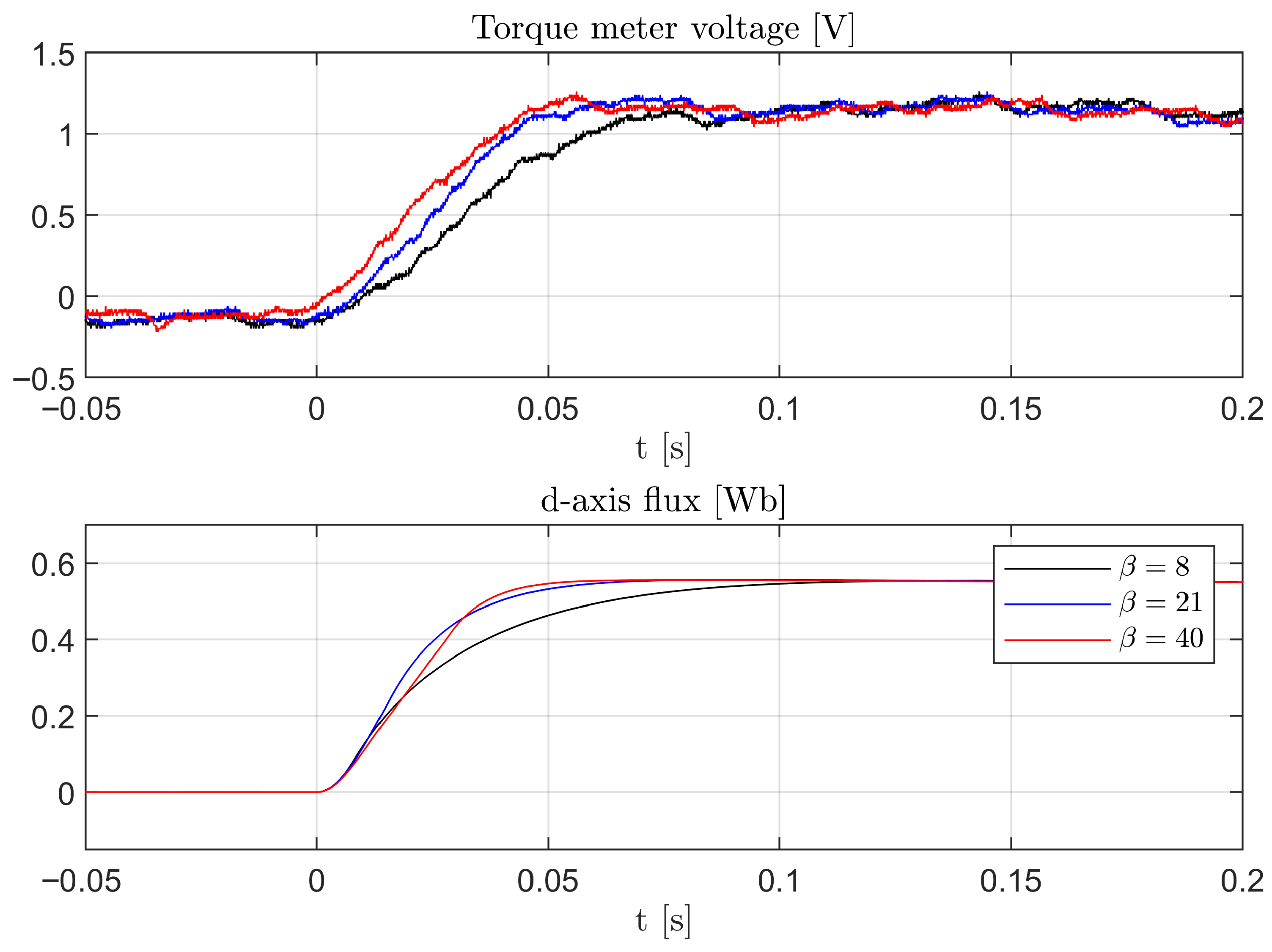The results are presented in Figure 6, Figure 7, Figure 8 and Figure 9.

An important thing is that the q-axis current control method is robust and independent from the d-axis control. None of the conducted tests show any important changes in the q-axis current behavior. The only exception is the additional harmonic occurring in the $i_q$ plot for ${\omega }_r=72.4{\displaystyle \frac{\mathrm{rad}}{\mathrm{s}}}$. This is, however, caused most probably by the speed measurement delay, which is relatively more significant for higher speeds. This, combined with the switching action realized by the control law, causes the chattering that could be eliminated with multiple methods.

Proceeding to the main focus of the paper, although very slightly, the d-axis current plots obtained for different motor speeds vary during the reaching phase. This behavior is natural and expected. It is the consequence of the non-ideal motor identification, which is inevitable in practice. However, when the sliding manifold is reached, the differences between subsequent plots vanish entirely.

The maximum current values obtained for the tests with three different speeds differ slightly and are approximately equal to $6.2\mathrm{A}$. Nonetheless, they are not equal to the predicted value, which, as one may read from Figure 3, is equal to $6.75\mathrm{A}$. This also happens due to limited parameter identification accuracy.

Regarding the IM flux values, one may notice that the q-axis flux always begins to rise after the control is engaged. This phenomenon signifies that the synchronization of the dq-frame with the d-axis flux is lost. Unfortunately, it is not possible to avoid due to the slip definition given in (2). During the initial phase of the control process, when ${\psi }_d\approx 0$, the value of ${\omega }_{sl}$ calculated with this formula tends to infinity. Because of this, it is necessary to limit the value of slip, thereby causing a temporary desynchronization. The dq-frame regains its proper orientation as it follows from (3).

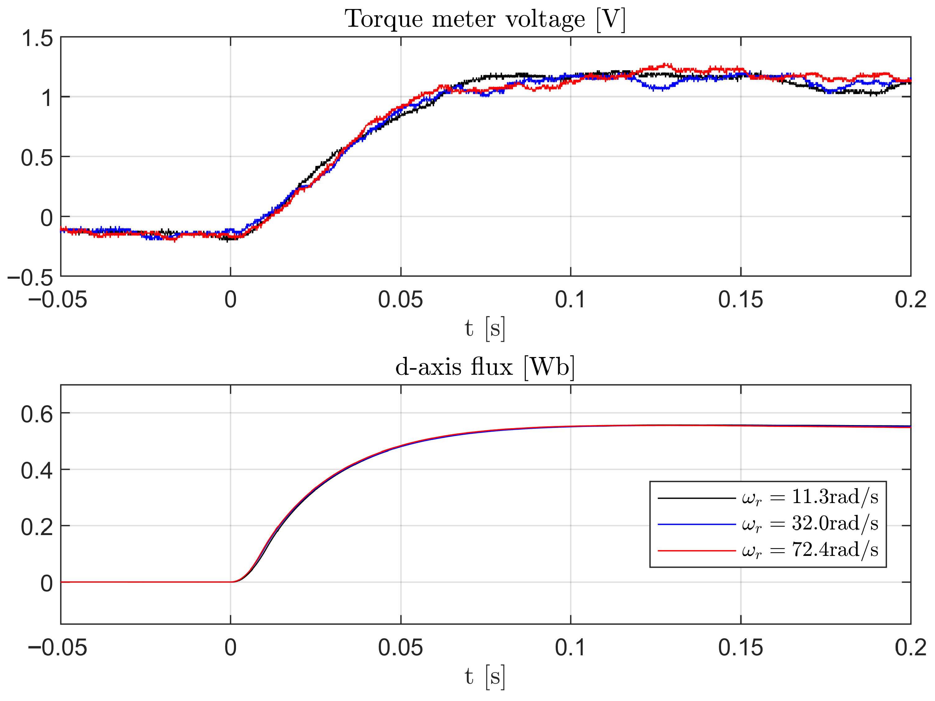
As it was stated earlier, when ${\psi }_q=0$ and $i_q=\mathrm{const}$, the IM torque is proportional to the d-axis flux ${\psi }_d$. The effect of the desynchronization impacts the torque transient response, which is why its shape differs from the ${\psi }_d$ plot. The two shapes are compared in Figure 7.

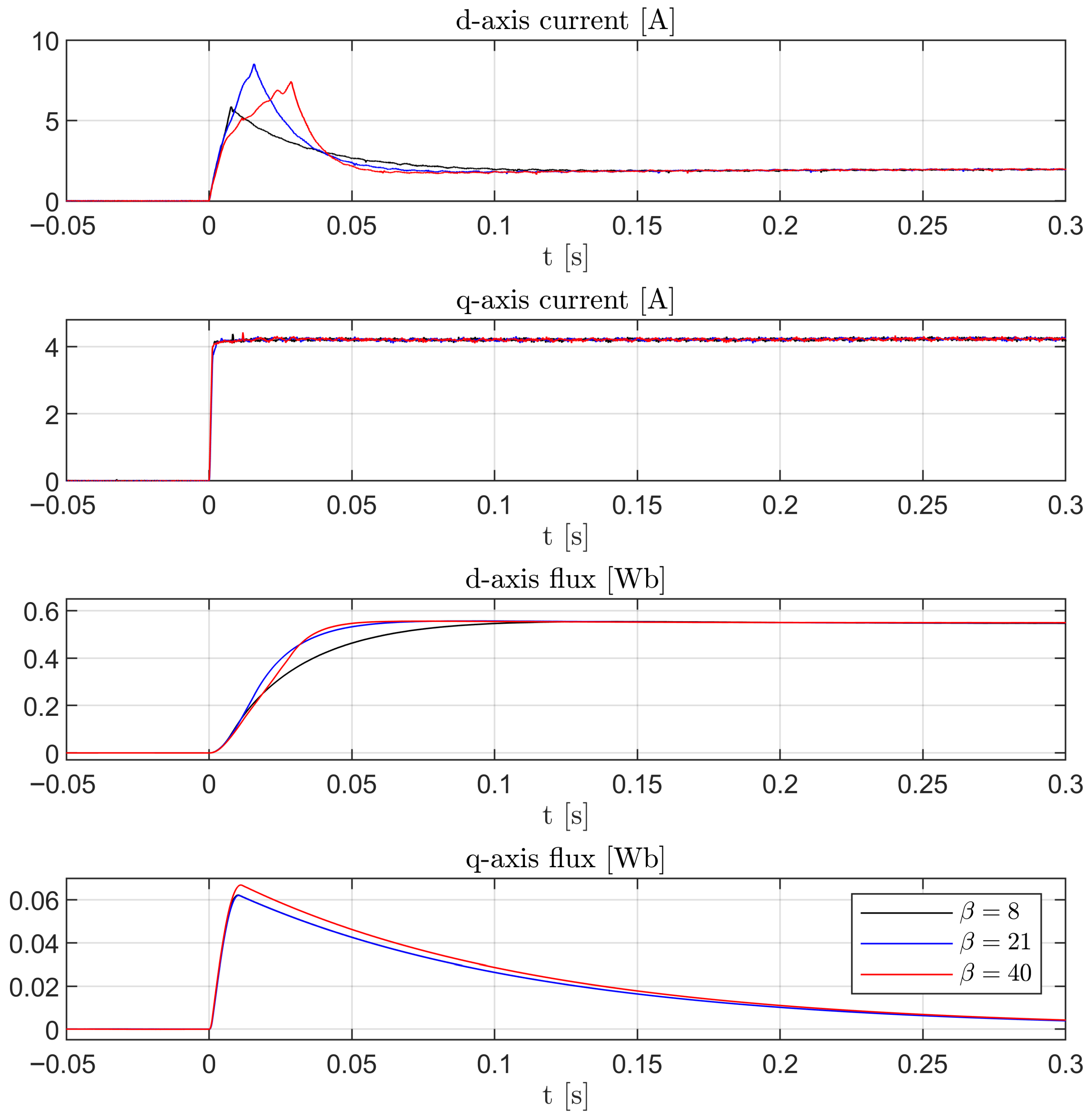
Most of the above conclusions also apply to the second experiment performed for three different values of the parameter $\beta$. There are two important aspects of the second test.

Firstly, it proves that the theoretical predictions considering the maximum current values are true in the sense that it cannot exceed a certain value for a given value of ${\gamma }_d$. It is visible by comparing the d-axis current plots obtained for $\beta =21$ and $\beta =40$, as the maximum current value decreased for larger $\beta$. This implies that the current cannot be increased beyond a certain limit by changing the value of $\beta$ and it makes the proposed algorithm safe in a certain sense.

Secondly, the d-axis plots show that the flux time constant is noticeably impacted by the change of the parameter $\beta$. This change seems more evident for smaller values of this parameter. One may notice that the torque dynamics is also accelerated by increasing $\beta$.

6. Conclusions

This paper presented an application of a sliding mode control for IM torque control employing new sliding manifold definition. It was shown that defining the d-axis sliding variable as a linear combination of the d-axis current and the d-axis flux errors can accelerate the IM torque transient response. Moreover, it was shown, that the reference d-axis current is reached with zero steady-state error.

For the q-axis current control, a well-known time-varying sliding mode was used. It was shown that this type of control grants fast response of the q-axis current and therefore almost entirely mitigates its impact on the torque dynamics.

The presented method was thoroughly analyzed in both theory and practice. The theoretical predictions were confirmed with reasonably limited accuracy. One of the issues worth exploring in the future is to find an optimal value of the $\beta$ parameters. Also, some reaching laws could be used to achieve even better performance of the presented torque control method.