Article

Heat Transfer Mechanisms in Refrigerated Spaces: A Comparative Study of Experiments, CFD Predictions and Heat Load Software Accuracy

1
Lisbon Superior Institute of Engineering, R. Conselheiro Emídio Navarro 1, 1959-007 Lisbon, Portugal
2
UnIRE, ISEL, R. Conselheiro Emídio Navarro, 1, 1959-007 Lisbon, Portugal
3
MARE-IPS, Marine and Environmental Sciences Centre, Escola Superior de Tecnologia, Instituto Politécnico de Setúbal, Campus do IPS—Estefanilha, 2910-761 Setúbal, Portugal
4
Faculty of Engineering and Sustainable Development, Department of Building, Energy and Environmental Engineering, Gävle University, 80176 Gävle, Sweden
*
Author to whom correspondence should be addressed.
Energies 2025, 18(23), 6280; https://doi.org/10.3390/en18236280 (registering DOI)
Submission received: 26 September 2025 / Revised: 4 November 2025 / Accepted: 13 November 2025 / Published: 29 November 2025
(This article belongs to the Section J1: Heat and Mass Transfer)

Abstract

A correct cold room heat load calculation ensures that the refrigeration system operates efficiently, reducing operating costs while maintaining a constant temperature to prevent stored goods from spoiling. Refrigeration engineers typically use software to size equipment such as expansion devices and evaporators and to estimate heat loads in cold rooms. These tools are available for free from refrigeration manufacturers or can be purchased from software developers. Although practical and easy to use, most of these programs do not follow the American Society of Heating, Refrigerating, and Air-Conditioning Engineers (ASHRAE)-recommended approach for estimating heat loads. This article evaluates heat transfer mechanisms, especially natural convection in a refrigerator, through experimental and CFD simulations. Depending on the expression used, the estimated convection heat flux at the evaporator ranged from 5.3 W to 14.2 W in case 0-N, 7.7 W to 25.1 W in case −10-N, and 5.1 W to 22.4 W in case 0-Y. Compared to convective heat transfer, radiation heat flux estimations are often more consistent across different expressions. The results from validated simulations were used to assess the performance of cold room heat load estimation software. Differences of up to 236% in heat load estimates were reported between the results.

1. Introduction

A common occurrence during food storage is natural convection. It can take place, for instance, while food is being transported in a container, stored in an unventilated cold room or kept in a home refrigerator. In reality, high temperatures are commonly found in the cold chain, especially in home refrigerators, where food is stored for the longest periods.
There are two varieties of household refrigerators on the market: vented and static. In Europe, the static system (without ventilation) is widely used [1].
When designing and operating a refrigerator, fluid mechanics and heat transfer work together as essential tools for the designer. Understanding air temperature and velocity profiles in refrigeration equipment is essential for maintaining food quality. When the consumer is aware of where the warm and cold areas are in the refrigerator, the items can be positioned appropriately [2,3]. It is common for a professional working in the food retail industry to know from experience where the colder spots are in a refrigerator or a cold room. It is also crucial to understand the thickness of the thermal and hydrodynamic boundary layers near the evaporator and other walls. If the product is too close to the evaporator wall, freezing can occur, and if it is too close to warm walls, the products can be deteriorated [3].
The airflow pattern and heat transfer behavior inside a static refrigerator present similarity to the enclosed cavity approximation. Therefore, research on enclosed cavities with different boundary conditions can be used to understand the thermal–fluid behavior of the static refrigerator [4,5,6]. The Particle Image Velocimetry visualization performed on static refrigerators under actual operating settings further supports the numerical studies’ suggestion that circular flow occurs inside the static refrigerator [7]. The warm air shifted towards the chilly wall at the top of the refrigerator.
If the Rayleigh number Ra > 103, the buoyancy-driven flow initiates natural convection heat transfer. Most studies suggested that the Ra for the static refrigerator varies between 108 and 109, indicating a buoyancy-induced laminar flow (Ra < 109) [8,9], thus promoting natural convection heat transfer. If this is the case, one can notice that a stagnant region of flow occurs at the central zone of the cavity, leading to a nonhomogeneous temperature distribution. This phenomenon can be a concern for food safety and quality.
Engineers tend to use software for the estimation of heat loads and sizing equipment. These are available from suppliers, manufacturers and distributors of refrigeration, but they can also be available from independent software developers. The biggest advantages of utilizing such software are the substantial time savings and improved accuracy. Software makes it possible to quickly determine critical load data for refrigeration equipment sizing. Computational Fluid Dynamics (CFD) simulations are thought to be particularly accurate for performing heat transfer calculations, despite their complexity and time-consuming nature [10].
The understanding of heat transfer in refrigeration appliances is crucial when studying new and more complex systems. Boeng and Gonçalves [11] investigated the effects of incorporating heat storage material (HSM) into the natural-draft condensers of household refrigerators. The heat transfer coefficient between the refrigerator exterior walls and the environment used in this study ranges from 10 to 15 W/m2 °C. The incorporation of a heat storage material in the natural-draft condenser of refrigerators ensures a relatively steady heat transfer throughout the operational cycle, contrasting with the intermittent transfer characteristic of a purely cyclic regime. The authors concluded that connecting the HSM to the heat exchanger, when performed properly, results in a better system performance than an uncoupled arrangement.
Gowreesunker et al. [12] examined the thermal performance of a 300 L freezer using Computational Fluid Dynamics. The CFD model was validated against experimental data and then utilized to calculate the freezer’s temperature stratification, heat transfer rates and heat transfer coefficients. The results show that internal heat transfer coefficients varied between 1.2 and 43.6 W/m2 °C, depending on the surface considered.
In a work by Zhang and Lian [13], the effects of shelves and food were analyzed on the temperature distribution and air circulation in three refrigerator configurations: empty; empty with shelves; and a loaded refrigerator with food stored. They used numerical simulations to solve laminar Navier–Stokes equations using a finite volume method. The Boussinesq approximation was used to model natural convection. Comparisons were made with and without radiation, the former using the discrete ordinates method. The results showed that radiation significantly changes the temperature distribution and air circulation pattern.
Muneeshwaran et al. [14] provide an extensive analysis of heat transfer modeling in various types of refrigerators, such as static, brewed, ventilated and side-by-side. They suggest a methodology to estimate the capacity of refrigerators under both loaded and unloaded conditions. Among other conclusions, the authors point out that temperature non-uniformity inside the refrigerator can lead to higher energy consumption and that the temperature distribution is strongly correlated with the air circulation inside the refrigerator. They also report that the temperature distribution in the refrigerator is mainly influenced by various design and operational factors, including the shelf arrangement, compressor on/off cycle pattern, thermostat settings, evaporator design, ambient conditions, door opening frequency and product loading temperatures.
Dhiwar and Khute [15] compared the results of the heat load calculation in a cold room, comparing two methods: CFD simulations and analytical calculations. They found a difference of 10% between the results yielded by the two methods. A heat transfer coefficient between the cold wall and the environment of 8.5 W/m2 °C was adopted in this study.
Accurate cold room heat load estimation guarantees the efficient operation of the refrigeration system, minimizing operational costs and environmental impact while maintaining a stable temperature to prevent the rotting of stored items. While some software tools follow the methodology recommended in ASHRAE for heat load estimation, most software packages do not meet this compliance, or the information about the methodology used in the calculations is not always available from the developer. This goes against, for example, what is practiced in the HVAC/building sector, where Building Energy Simulators must comply with the methodology defined by ASHRAE for design and annual energy analysis.
While it is true that a lot of research has been performed on heat transfer in refrigerators, little has been written about assessing the effectiveness of the software used to calculate heat loads in refrigeration. In this area, very few works have been published comparing the results obtained from traditional thermal load calculation software with Computational Fluid Dynamics (CFD) simulations. Most studies focus either on detailed CFD modeling for the analysis of temperature distribution and airflow patterns [9,16] or on the use of analytical and semi-empirical [17,18] methods for equipment sizing. However, a direct comparison between these two approaches remains scarce in the literature.
Most of the available literature tends to focus on either CFD-based modeling or on simplified analytical tools, but seldom both in a comparative framework.
Nonetheless, a few studies in adjacent fields have explored this gap. For example, Wang et al. [19] proposed a combined CFD and thermal–hydraulic modeling (THM) approach to evaluate the cooling of oil-filled transformers. Both models were validated against experimental heat-run tests, showing good agreement. While CFD provided higher accuracy, THM proved to be faster and more suitable for day-to-day engineering practice.
Similarly, Wang et al. [20] developed a simplified cooling load calculation method for stratified air-conditioning systems, using an equivalent heat transfer coefficient. When compared to CFD simulations, the simplified method produced a load estimation deviation of only ~4%, supporting its reliability for practical use.
In the refrigeration context specifically, Nkwocha et al. [21] used CFD to analyze the cooling capacity of a refrigerated container, particularly as a function of the initial product temperature. Although this study relied solely on CFD, it provides insight into the level of detail achievable with such simulations. On the other hand, Marques et al. [22] combined theoretical modeling and experimental validation to study a thermal energy storage refrigerator, though a direct comparison with commercial load calculation software was not included.
In the HVAC domain, more comparative studies are available. Beghelli et al. [23] assessed the discrepancies between several Building Energy Simulation (BES) tools such as EnergyPlus, TRNSYS and IDA ICE. Although annual load predictions were similar (errors between 0.1% and 5%), hourly deviations reached normalized RMS errors between 35% and 50%, well above the ASHRAE Guideline 14 thresholds. This highlights the potential limitations of relying solely on software outputs without further validation.
Other notable examples include a Brazilian study [24] which compared OpenFOAM-based CFD analysis with proprietary HVAC software to assess thermal comfort through metrics like ADPI, and a review on CFD–BES coupling, which discusses hybrid approaches that integrate detailed airflow simulations with building-level energy modeling. Similarly, Chowdhury et al. [25] analyzed cooled beam systems in retrofitted buildings using an integrated CFD–energy simulation approach.
Despite these efforts, the specific comparison between CFD and commonly used refrigeration load calculation tools remains poorly documented, especially in the context of domestic or commercial cold storage systems. This scarcity points to the need for targeted research assessing the reliability, applicability and limits of each approach across a range of realistic refrigeration scenarios.
This lack of studies represents an important knowledge gap, as the choice of the calculation method can significantly influence the predicted cooling loads, temperature uniformity and overall system performance. Thermal load calculation software, while widely used in industry for its speed and simplicity, often relies on standard assumptions and may overlook the complex thermal–fluid interactions present in real systems. CFD simulations, on the other hand, can capture these phenomena in greater detail but are time-consuming and computationally expensive.
A systematic comparison of these two approaches would not only help validate the accuracy of commonly used software but also provide guidelines for when CFD analysis is truly necessary and when simplified tools are sufficient. Filling this gap would ultimately support more reliable refrigerator design, improved energy efficiency and a better preservation of stored products.
This article assesses the outcomes of heat transfer mechanisms, particularly natural convection in a refrigerator, at the same time comparing the performance of heat load estimation between cold room software using validated CFD simulations.
The study has two main objectives. It analyzes convection and radiation heat transfer coefficients in an evaporator using heat transfer theory expressions and compares these to the same variables calculated numerically with CFD. Additionally, it evaluates the performance of heat load software tools using a validated CFD model. Experimental data from [1] are used for validating the numerical code. Tests were conducted on a full-scale refrigerator model. Validated simulations were then employed to predict the temperature and velocity profiles for three cases. The refrigerator’s geometry and test ambient conditions remained constant during the simulations.

2. Materials and Methods

2.1. Refrigerator Model

To validate the numerical results, a set of reliable and high-quality experimental data was necessary.
A refrigerator model with dimensions 0.5 m × 0.5 m × 1 m (length × width × height) was constructed by [1]. It has three vertical walls composed of double glass walls and one vertical aluminum wall. A cooling coil is placed inside the latter, where a low-temperature water–glycol mixture is used to maintain a constant temperature in this aluminum wall, circulating inside a loop pipe. The top and bottom horizontal walls are made of PVC (thickness: 2 cm). All external walls are insulated using expanded polystyrene plates (thickness: 4 cm). Air temperature was measured using calibrated T-type thermocouples (precision ± 0.2 °C).
Specific test conditions required that the empty cavity is filled with objects representing the food loading. For that purpose, the model was filled with 4 blocks of hollow PVC spheres. The diameter of each sphere was 7.5 cm, and each block was composed of 6 × 5 × 3 spheres. Spheres are, in this case, considered airflow obstacles only, and they may be considered adiabatic. They may alter the air temperature field, though. The position of these thermocouples was the same as that of the empty case. For the identification of test cases, coding notation will use the information of the cold wall temperature and the existence or absence of internal objects. Case 0-N corresponds to a refrigerator with a wall temperature set at 0 °C (parameter “0” in the case name), in which the compartment is empty (letter “N” for no spheres). Case −10-N corresponds to an empty refrigerator with its cold wall maintained at −10 °C, and case 0-Y to a test where hollow spheres have been put inside the refrigerator and the wall was kept at 0 °C. Table 1 illustrates the three cases studied as well as the conditions of each test.
Tests were carried out in a controlled temperature room set at 20 °C for all experiments. Two temperatures were set at the cold wall: 10 °C and 0 °C. These two temperatures mimic the evaporator temperature at the beginning and end of the compressor work cycle, respectively. Time was given for the steady state regime to be reached for all experiments, i.e., until the internal air temperature became constant. Then, a time-averaged air temperature was calculated at each measured point.
Table 2 shows the dimensions of the model and the locations of the thermocouples. In Table 2, Plane 1 is used as a reference for the placement of the thermocouples, which will measure the temperature profiles over the height of the refrigerator.

2.2. The CFD Model

Analytical solution techniques are typically confined to idealized problems involving simple geometries [26]. As a result, Computational Fluid Dynamics (CFD) software has become an indispensable tool for investigating more complex and realistic scenarios in fluid mechanics and heat transfer. The physical phenomena involved in an empty and a filled refrigerator are characterized by complex mechanisms like natural convection, radiation, the co-existence of turbulence and laminar zones and unsteadiness, thus the preference for using CFD methods in this investigation. For this numerical study, a commercial CFD code, Ansys-Fluent (version 2025 R1), has been used to predict variables like air temperature, wall temperature, heat flux rate and velocity vectors in a domestic refrigerator. Figure 1 shows an overall picture of the refrigerator model used in the simulations for the case 0-Y (a), as well as the mesh generated for case 0-N (b).
The data have been obtained from solving the mass, momentum and energy equations. Furthermore, additional quantities from turbulence models were used, because of the Reynolds Average Navier–Stokes approach. Equations were extended to the 3rd dimension in space.

2.3. CFD Set-Up

2.3.1. Turbulence

Turbulence is a complex problem that must be tackled. It mainly affects numerical analysis, although it might also introduce uncertainties in experimental analysis [27,28]. Although the Ra of the tests considered is found to be below the critical transitional regime of Ra < 109, turbulence zones are expected to be encountered away from the walls, e.g., inside the cavity. The standard k-ε was the model selected in this study due to the good performance achieved in similar applications. This model has been widely used in studies of fluid mechanics and heat transfer [29]. The CFD code’s default turbulence model constants remained unaltered. Although more accurate predictions can be obtained by refining the mesh in this zone and selecting a suitable turbulence model, such as a low Reynolds number turbulence model, the law-of-the-wall is typically used to avoid a very fine mesh near the solid boundaries [30]. Fluent automatically switches to a low Reynolds turbulence model if y+ = 1 at the cell in the vicinity of the wall. To achieve a higher degree of accuracy in the simulations performed, this condition must be verified in every test simulated. Results of the calculated wall parameters are shown in more detail in Section 2.3.5.

2.3.2. Buoyancy

The air’s density will change as a result of the temperature rise when heat transfer is convected to the air [31]. The particles will then be induced to move by the gravitational pull acting at various intensities. Fluent software allows for the numerical modeling of natural convection. The Boussinesq method is typically used in certain situations. With the exception of the momentum equation, this approximation assumes density as a constant. The density parameter will be represented as a function of temperature in the equation: (ρρ0)g ≈ −ρ0 β(TT0)g. Here, ρ0 designates the reference air density and T0 the temperature under study, β the air expansion coefficient and g the gravitational acceleration. This approach produces results with acceptable deviations if the variations in the air temperature comprise β(TT0) << 1.

2.3.3. Radiation

In the presence of heat transfer by natural convection, the radiation component may represent a significant fraction of the heat transferred [26]. Therefore, the radiation emitted and absorbed by surfaces will condition the final balance of energy. The discrete ordinates model was selected when performing calculations. In this model, the number of bands is specified to be zero, since the optical properties of the model walls do not change with the temperature. Regarding angular discretization, Theta and Phi divisions were each set to three. Air was considered a non-participating medium.

2.3.4. Boundary Conditions

The definition of boundary conditions represents an important part of the formulation of any problem to be solved by a CFD code [30]. The boundary conditions were defined to describe appropriately the physical conditions of the experiments. Each boundary condition is defined in Table 3 and Table 4 for each case considered.
The “wall,” or, more specifically, the “Near wall treatment” boundary condition, is used to define the fluid–solid interface. Walls were defined considering losses from convection and radiation. The heat conduction is calculated using the Ansys-Fluent software for solid domains. For this purpose, a thickness was defined for these surfaces, along with the definition of a material. Table 5 shows the specification and properties of every material considered in simulations.

2.3.5. Grid Generation

The test equipment was represented in a simplified geometric model that was utilized in the CFD simulations. To model the interior domain of the refrigerator cavity, tetrahedral elements were employed generally, whereas hexahedral elements were preferred close to the walls.
When modeling the boundary layer, inflation was created in the fluid domain, namely in the interfaces with solid domains, using a transition ratio of 1.2.
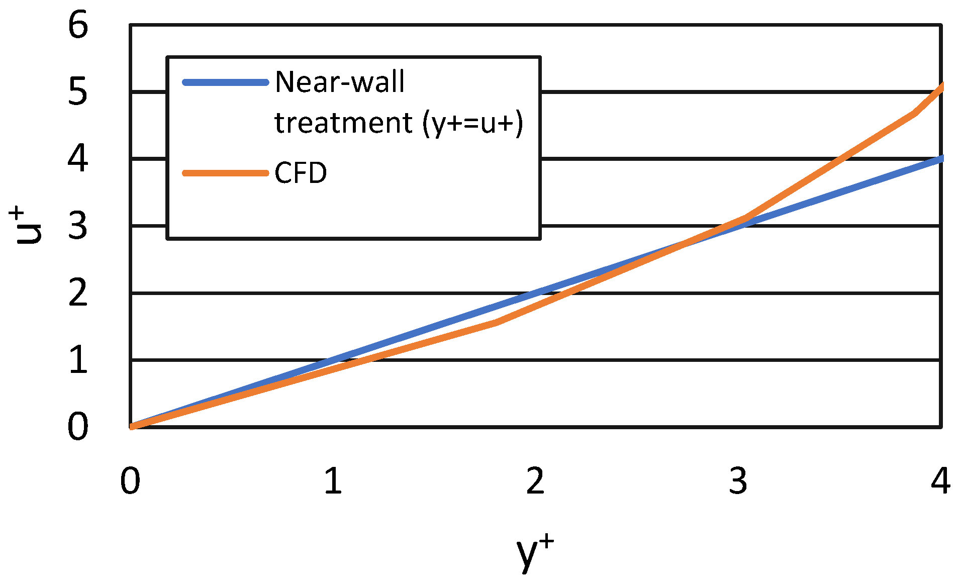
To specify the thickness of the first cell, the calculated nondimensional distance to the wall y+ was compared to the same parameter but obtained using the law-of-the-wall model at the viscous sublayer. To calculate the nondimensional distance to the wall, the velocities of air on each cell, the distance to the wall and the shear stress at the wall were necessary. These variables were extracted from the CFD results on the vicinity of the wall, i.e., comprising the first five cells. This distance represents the first 4 mm of the mesh close to the wall. For the calculation of the friction velocity, the shear stress was also obtained through CFD calculations. Figure 2 presents the relationship between the calculated velocity profile and the log-law near the cold wall in a cell located at (x,y,z) = (0,250,500) mm and assures us that the thickness of the first cell was correct.

2.3.6. Grid Independence Study

To achieve a compromise between calculation time and result accuracy, a mesh refinement study was conducted. Temperature was selected as the variable for the mesh independence study, since it is a crucial parameter in this investigation.
Table 6 shows the air area-weighted average temperature in a plane at x = 250 mm for four different mesh sizes for case 0-N. The area-weighted average of a quantity is computed by Fluent by dividing the summation of the product of a selected field variable and facet area by the total area of the surface:
1 A ϕ d A = 1 A i = 1 n ϕ i A i
ϕ is the variable under study, in this case, the temperature. Table 6 also shows the TAWA applied to the experimental data at a plane of y = 127 mm in order to compare the results from weight-averaging the temperatures from simulations with the experiments from a spatial point of view. Differences between grid size simulations and the finest mesh were also represented by the variable ΔTAWA.
Differences in temperature are subtle, but still can be found by comparing the two coarsest meshes—comprising 24,254 and 55,456 elements. On the other hand, when the number of elements increases above a certain value, calculations provide close results, indicating that no further refinement of the mesh is necessary. A good quality mesh, together with a correctly placed first grid point at y+ = 1 was decisive to obtain the most accurate calculations. A mesh with 72,734 control volumes was selected to perform the calculations in case 0-N.

2.3.7. Numerical Solution Algorithm and Solver Settings

The 3-D model was created in Ansys Fluent. The finite volume method was used to solve the governing Equations (1)–(3) for the continuity, momentum and energy, respectively, in directions i and j = 1, 2, 3.
ρ ¯ t + x j ρ u ¯ j = 0
t ρ u i ¯ + x j ρ u i ¯ u j ¯ = p ¯ x i + x j μ u i ¯ x j + u i ¯ x j 2 3 δ i j u k ¯ x k + x j ρ u i ¯ u j ¯ + ρ g i ¯
( ρ c p T ¯ ) t + x j ρ c p u j ¯ T ¯ = x j λ T ¯ x j ρ c p u j ¯ T ¯ + q ˙ ¯
In the discretization of the convective terms of the momentum, energy and turbulence equations, the second-order upwind numerical scheme was selected. The solver was set to incompressible, steady-state and pressure-based types. The pressure–velocity coupling was determined using the SIMPLE algorithm. A convergence criterion was based on the unscaled residuals’ magnitude. Values of 10−3 were used for the residuals of continuity, momentum and turbulence, and 10−6 for the energy and radiation equations.

3. Results and Discussion

3.1. Case 0-N

3.1.1. Temperatures

Figure 3 shows the calculated and measured temperature profiles for case 0-N at thermocouple columns n° 4, 5 and 6, in three rows at z = 10 cm, z = 50 cm and z = 90 cm. The air temperature ranged between 0 °C close to the cold wall and 11 °C at the opposite wall. This distribution occurs because a circulation pattern in the air is present in the central part of the cavity of the refrigerator. The air descends along the cold wall due to density differences and rises when it is being warmed up close to the wall that is not refrigerated. The simulations reported temperatures between 0 and 10.2 °C at a height of z = 90 cm, showing a good correlation between the measured and simulated results. Thermal stratification is also noticeable inside the cavity: air reaches around 6 °C at the bottom of the refrigerator, at z = 10 cm, and about 11 °C in its highest zone at z = 90 cm. This phenomenon is expected to occur in an unventilated refrigerator where temperatures are known to be less homogeneous.
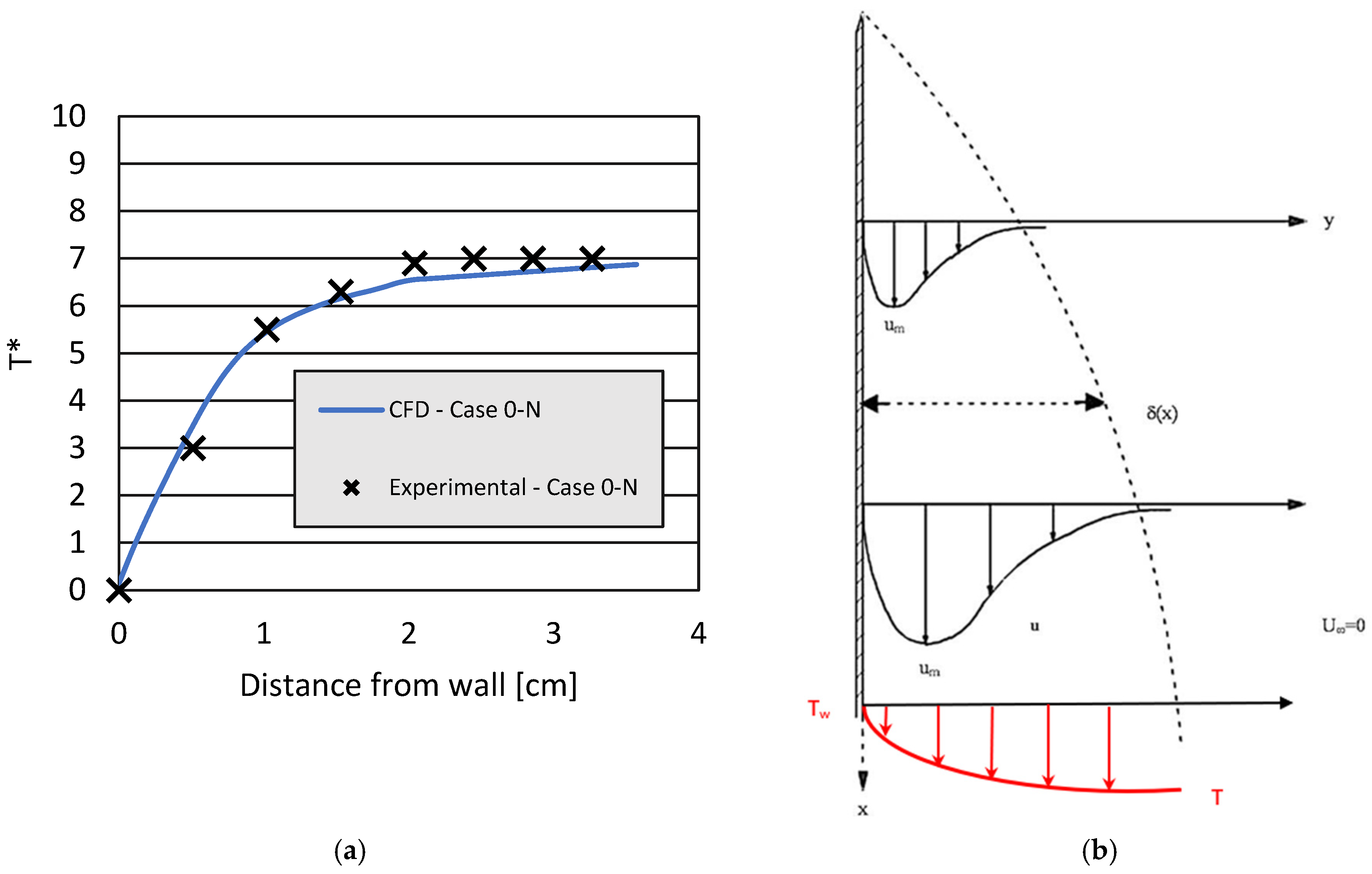
The influence of the boundary layer is also noticeable in the profiles of Figure 3 and resembles the theoretical thermal boundary layer profile when natural convection is present in the vicinity of a cold wall (Figure 4b). The temperature distribution close to the wall can be seen in Figure 4a. In this chart, the dimensionless value T* is used instead of the absolute temperature. It is given by the following:
T = T T c T a m b T c
In Equation (5), Tc is the interior temperature used in tests, i.e., 0 or −10 °C, Tamb is the lab temperature, 20 in the experiments, and T is the experimental temperature measurement.
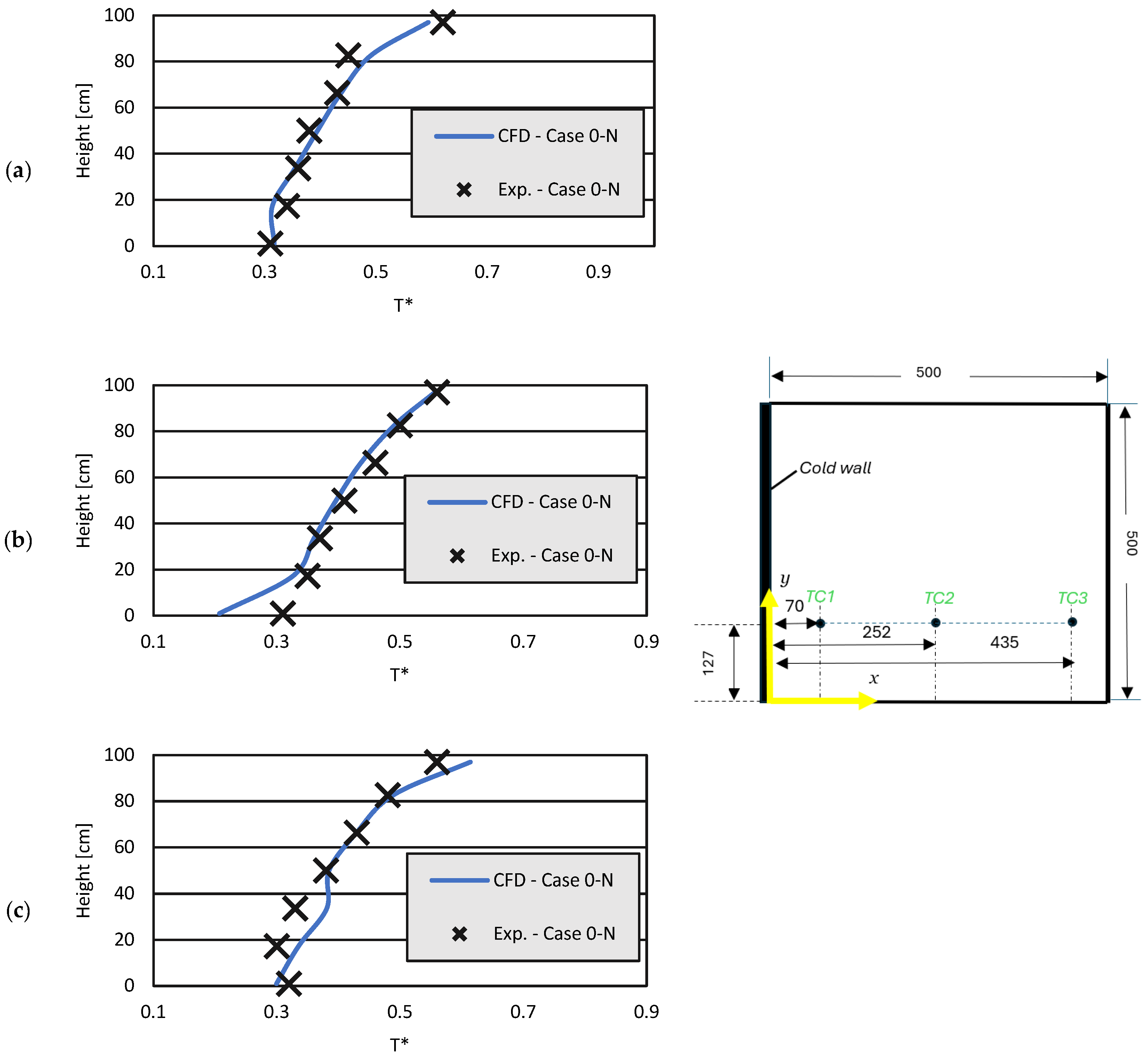
The predicted temperature profiles, as well as the measurements, are shown in Figure 5 for case 0-N along thermocouple columns 1, 2 and 3. The profiles show that a stratification is present inside the compartment of the refrigerator in case 0-N, as expected, as in the presence of natural convection inside a cavity. The non-dimensional air temperature differences between the top and the bottom of the refrigerator ranged between 0.7 and near 0.2, respectively. These differences may be attributed to air recirculation and air stagnation near the top of the compartment. A good correlation between the measured and simulated results is found in case 0-N. Absolute temperatures of 12.3 °C are found in thermocouple column nº 3 inside the refrigerator box near its ceiling, which may not be acceptable for food preservation.
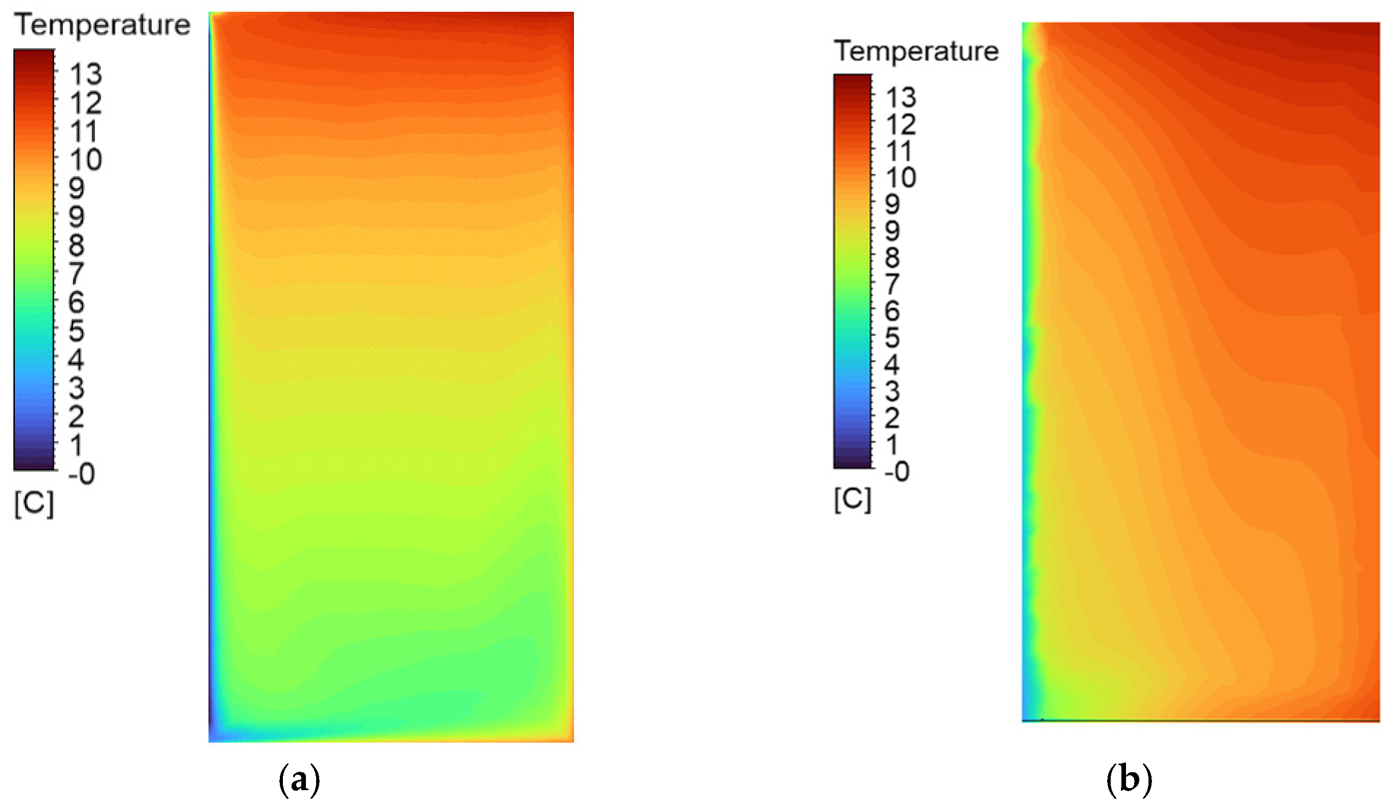
Figure 6 shows the air temperature contours of air at a plane of y = 250 mm and in a side wall at y = 0. In Figure 6a, the boundary layer near the cold wall can be spotted. It is growing in thickness towards the end of the wall, as expected. Stratification can be clearly noticed on the upper half of the compartment. Temperatures between 8 and 12 °C are reported in the top region and the lower half, with a more uniform temperature of around 5–6 °C. An impinging jet is also noticed when the cold air, which is descending from the plate, strikes the bottom of the refrigerator. Figure 6b shows the temperature contours on a side wall. Temperatures in this solid region are far more homogeneous compared to the air values. Most of the surface portion reaches around 10–11 °C. The influence of the cold wall is noticeable, as can be seen from the thin layer on the left side of the picture, next to it.

3.1.2. Air Velocity

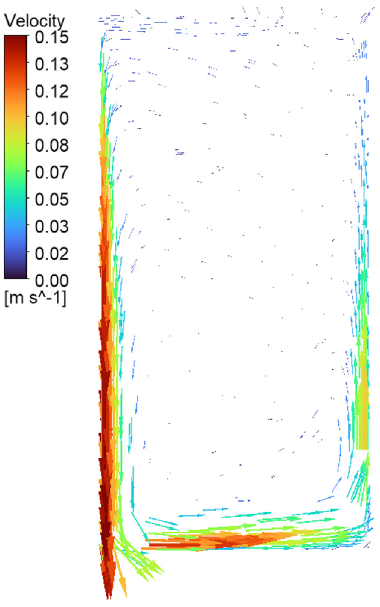
Figure 7 shows the predicted velocity vectors and magnitudes. A recirculation pattern is found by looking at velocity vectors, which are pointing down near the cold wall and pointing up at the opposite wall. This finding supports the previously discussed fact of non-uniform temperature distribution inside the food compartment. Zones near the cold wall show much higher velocities compared to the central zone. Not-so-high velocities are also encountered close to the other walls and near the floor of the refrigerator. The highest velocity gradients are clearly happening next to the cold wall. Magnitudes between 0.10 and 0.15 m/s are encountered in this region.
Natural convection heat transfer in a closed, small cavity like the one studied in case 0-N, aside from radiation heat transfer, is unlikely to provide a uniform distribution of air temperatures.

3.2. Case −10-N

3.2.1. Temperatures

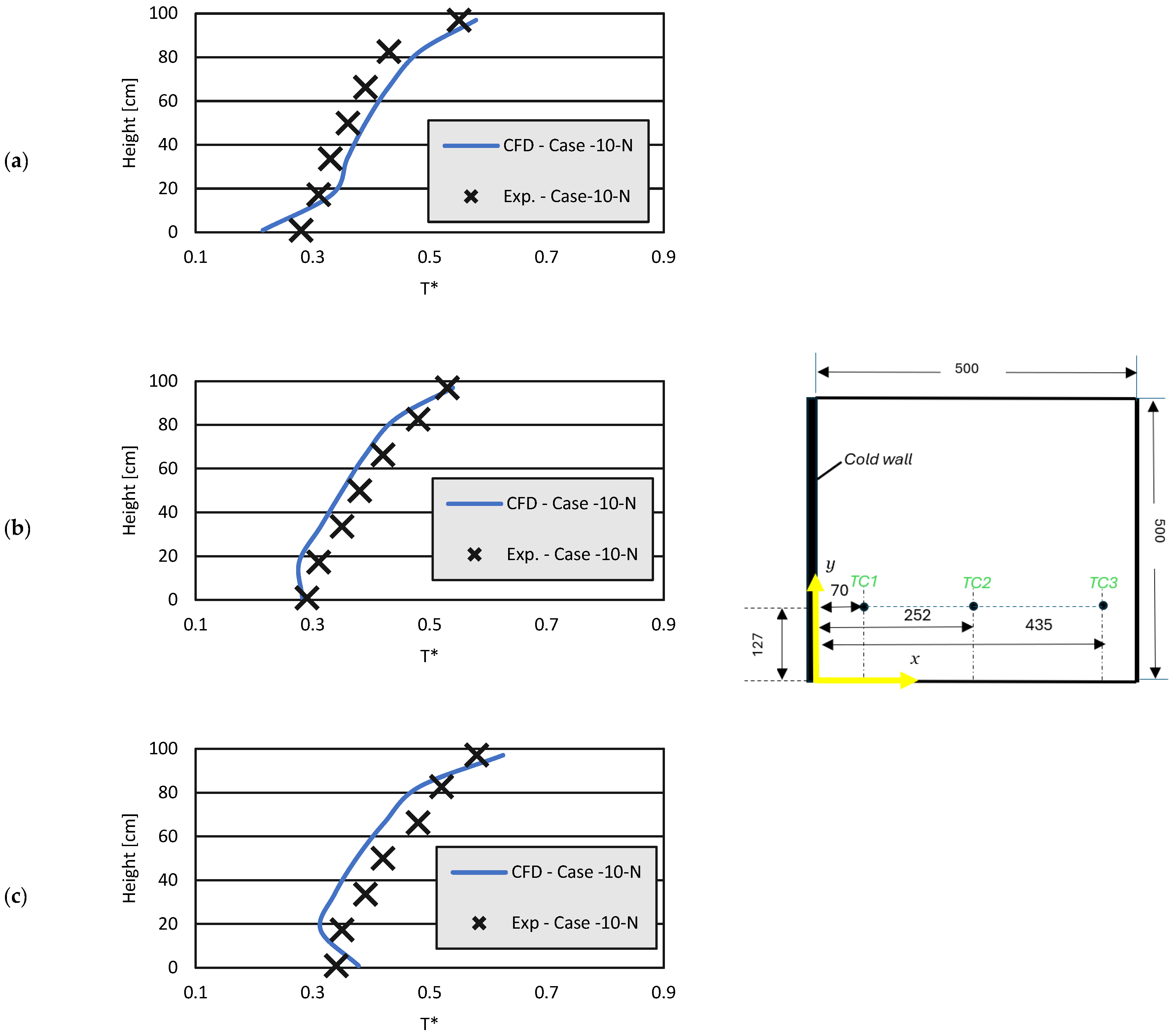
In case −10-N, the cold wall is maintained at −10 °C, representing the end of the compressor-on cycle. Figure 8 shows the calculated and measured temperature profiles for case −10-N over thermocouple columns 1, 2 and 3.
Lower air temperatures are found when comparing this to the 0-N case, as expected. Non-dimensional temperatures, T*, range from 0.2 at the bottom of the compartment to 0.5 at TC column number 1. TC column number 2 presents non-dimensional temperatures of 0.3 near the floor and around 0.5 at the top of the compartment. Looking at the lower half of profile (c), an inflexion is present in the temperature. Air, which tends to be cold near the floor, is showing that this is no longer the case in this TC column. Column 3 is placed on the opposite side of the cold wall. Air that is descending mixes with the air near the floor, elevating the temperature in this region. This fact is more notorious in TC column 3 than in columns 1 and 2 because of its proximity to the opposite wall. However, generally, stratification is still present in this case. Maximum absolute temperatures of 8.7 °C are found in thermocouple column nº 3, which may still not be acceptable for food preservation.
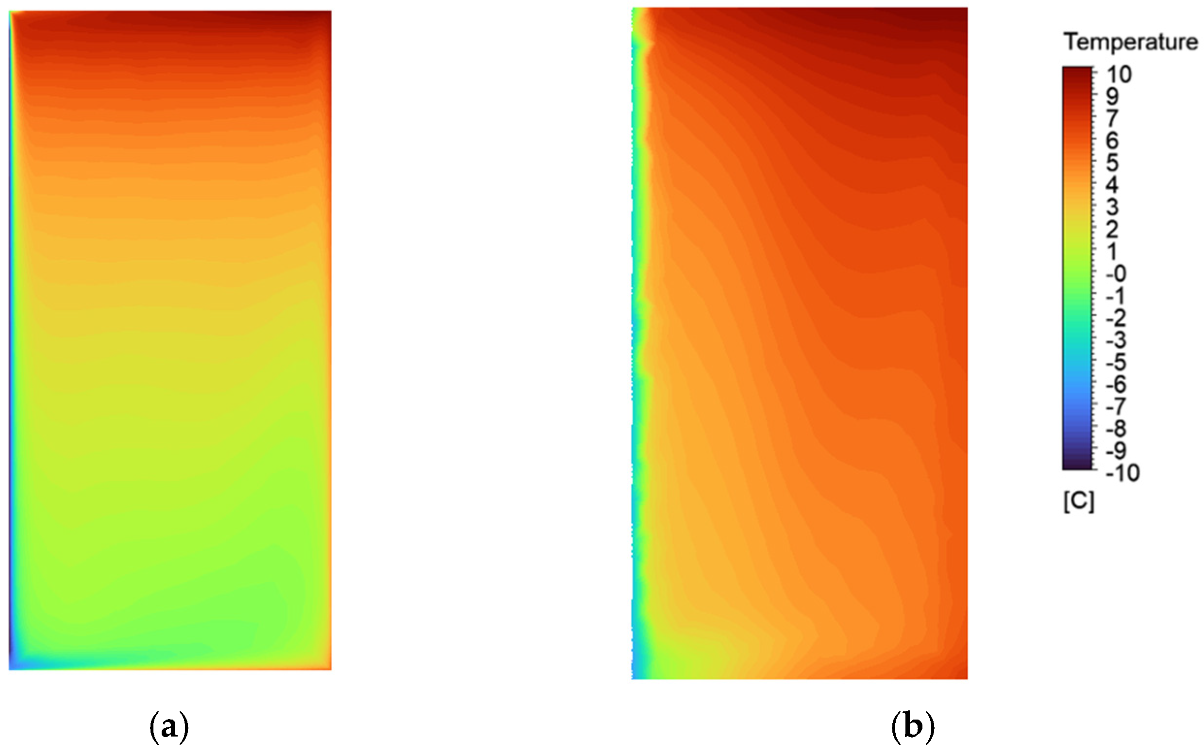
Figure 9 shows the air temperature contours of air at a plane of y = 250 mm and a side wall at y = 0. In Figure 9a, the temperature distribution is like case 0-N, discarding the difference in the magnitudes.
Figure 9b presents the temperature contours in a side wall. The diffusion of temperature in this solid region resembles the previous case 0-N, the main difference being the magnitude of the values. Here, the wall reaches around 5–6 °C on most of its surface.

3.2.2. Air Velocity

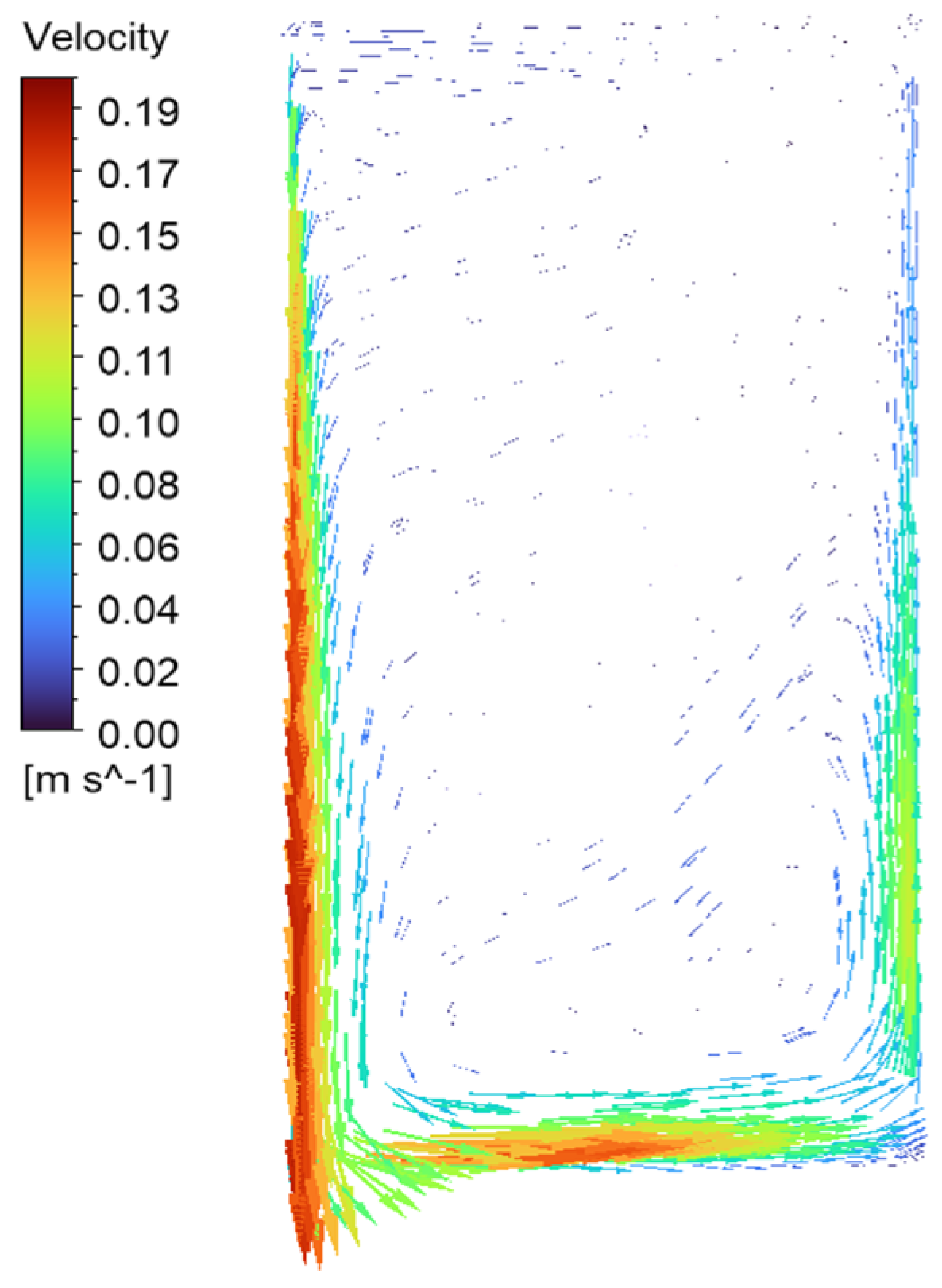
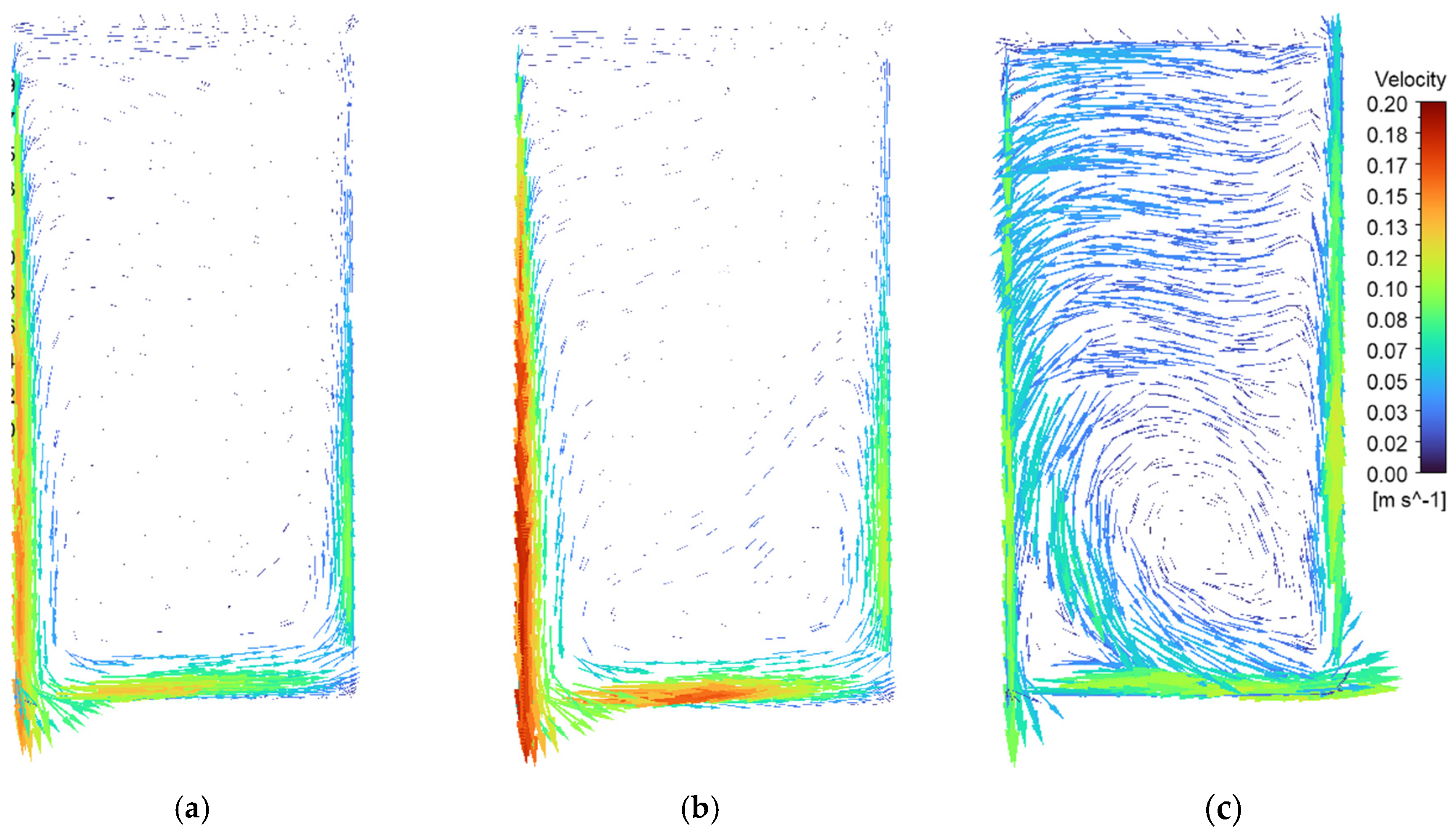
Figure 10 presents the velocity vectors and magnitudes for case −10-N. A circular pattern of flow, like that happening in an empty cavity, is observed. Comparing case 0-N and case −10-N, it can be noted that in both the velocity magnitude assumes higher values on the walls and is much smaller at the center of the cavity. The difference between magnitudes is also significant. Case −10-N presents maximum values of 0.19 m/s versus 0.15 m/s in the previous case. This has to do with the intensity of the temperature gradient between the wall and the air. However, stronger gradients have an impact on the velocity magnitude. Ra = 7.4 × 10⁸ is expected in this case, which characterizes the flow as laminar. In case 0-N, Ra = 5.1 × 10⁸ is predicted, which presents lower maximum velocities.

3.3. Case 0-Y

3.3.1. Temperatures

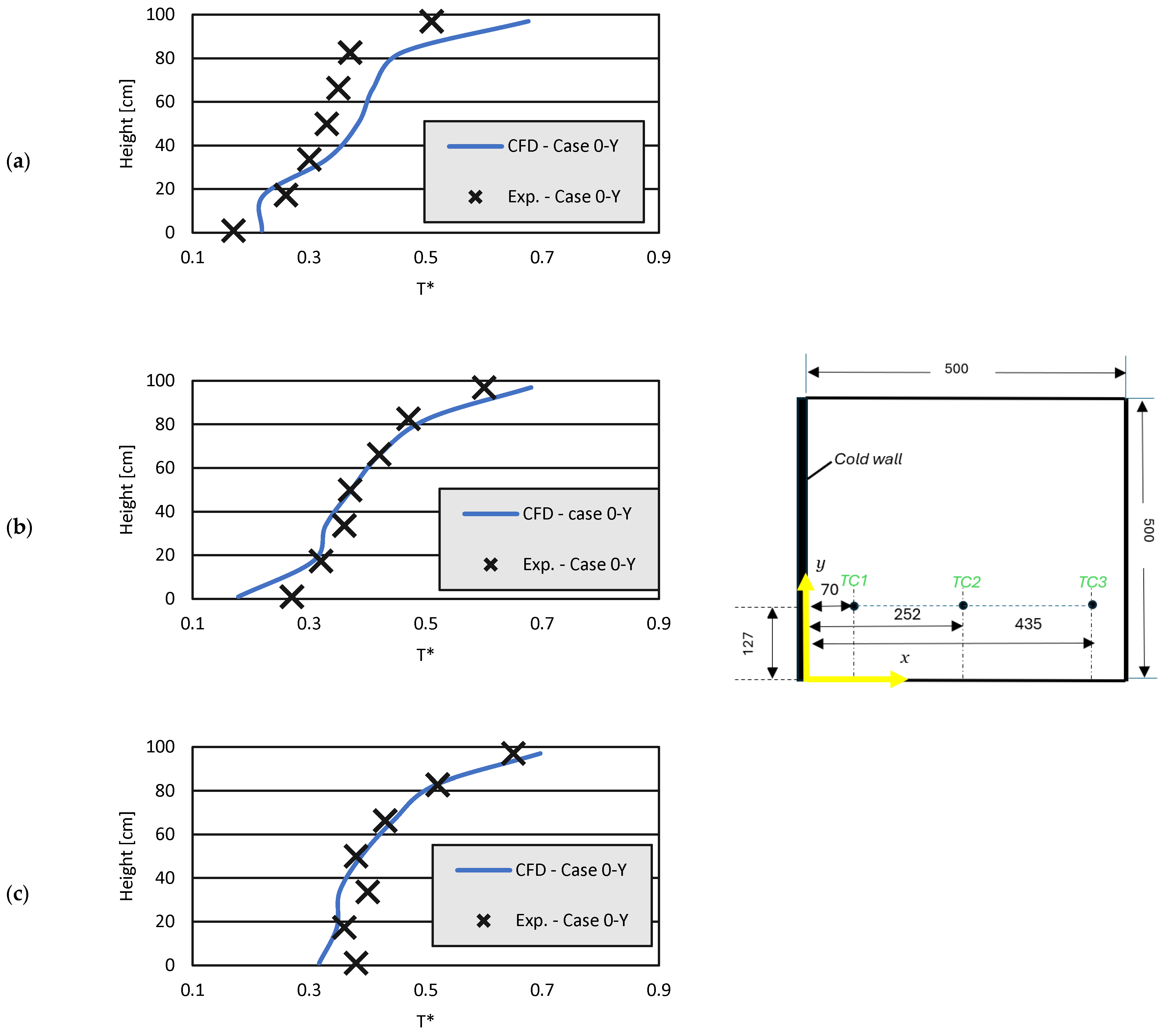
Case 0-Y represents an approach to a more realistic scenario and mimics the refrigerator compartment loaded with food. The cold wall is maintained at 0 °C. Figure 11 shows the calculated and measured temperature profiles for case 0-Y along thermocouple columns 1, 2 and 3.
Higher air temperatures are found on the top of the cavity compared to case 0-N. This is due to the barrier created by the spheres inside. Otherwise, temperatures are quite similar between the two cases at the remaining locations. A good agreement between CFD simulations and experiments is generally achieved. However, CFD is shown to struggle with the prediction in temperatures in thermocouple column number 1, namely on the top half of this column.
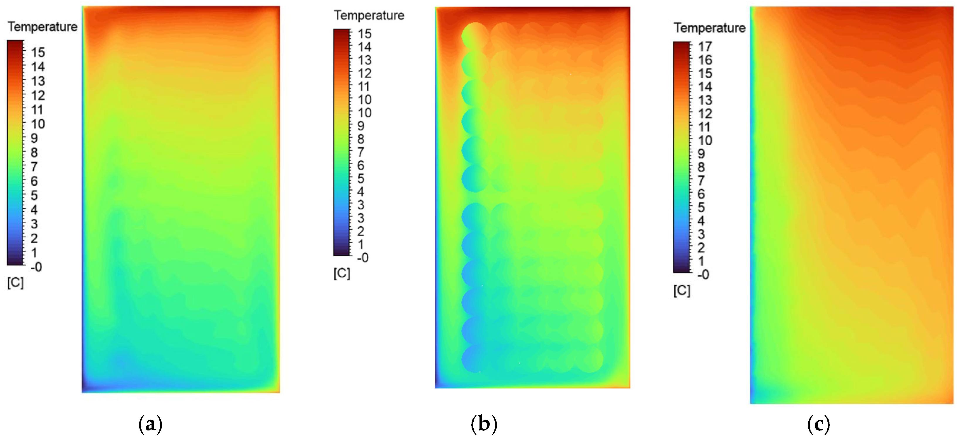
Figure 12 shows the air temperature contours of air at a plane of y = 250 mm and a side wall at y = 0. In Figure 12a, stratification is clearly more pronounced than in case 0-N, the cold wall being maintained at the same temperature of 0 °C in both cases. Differences of almost 14 °C are found between the top and the bottom of the compartment.
Figure 12b shows the temperature contours at a plane of y = 130 mm. Although the temperature magnitudes are similar to the previous discussed location (at y = 250 mm), in this region, the distribution of temperature reveals the concentration of a hotter spot in the upper half of the refrigerator. This might indicate that the cold air has more difficulty passing through the spheres, which leads to a less uniform distribution of temperature.
Figure 12c presents the temperature contours on a side wall. The distribution of temperatures is different compared to case 0-N, being less uniform here. The empty space between the spheres and the cold wall seems to provide room for air to descend along the cold wall, which causes lower temperatures at the wall.

3.3.2. Air Velocity

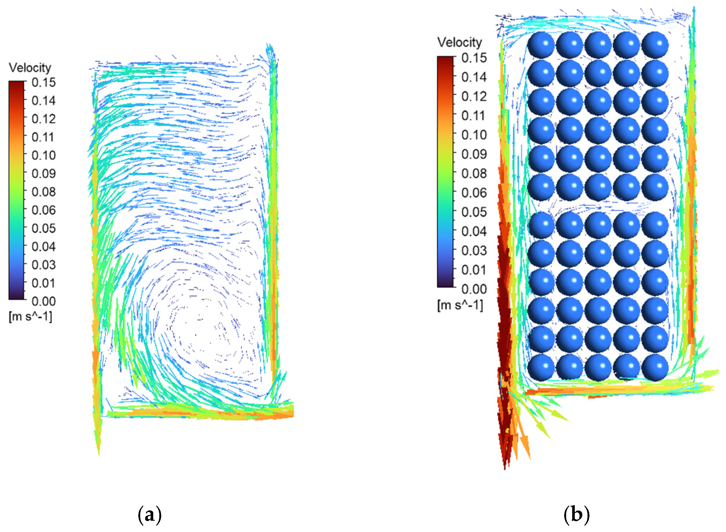
Figure 13a shows the velocity vectors and magnitudes in case 0-Y. Interestingly, air velocity distribution is far more uniform in the presence of obstacles inside the compartment. Compared to the empty cavity experiments, this arrangement results in lower velocities close to the walls and much higher speeds in the central zone. However, the velocity magnitude is typical of buoyancy-driven flows, since there is no forced mechanism in the case of static refrigerators. In Figure 13b, the velocity vectors are sketched in a selected plane located at y = 130 mm. In this section, the velocity vectors reach higher velocities next to the floor on the lower half of the cold wall. This is due to the fact that, in the space between the spheres and the cold wall, air has less room to pass through. In Figure 13b, it can also be noticed that, for the residual air speed magnitude around the spheres and in some of the spaces around them, the air is practically stagnated. Figure 14 shows the results in a unified scale of velocity for the three cases studied placed side-by-side for comparison purposes.

3.4. Heat Transfer

This study will also cover a heat transfer analysis for the three cases presented using a previously validated CFD model. The variables of interest in this discussion are the heat transfer coefficient and the heat flux rate. These two quantities are to be evaluated at the cold wall surface for cases 0-N, −10-N and 0-Y. Both radiation and convective components will be considered in the analysis. Several expressions are available for the estimation of the natural convection heat transfer coefficient in a cold vertical wall and are usually a function of Nu and Ra for the convective heat transfer. On the other hand, the temperatures of the cold and hot surfaces are normally defined for the calculation of the radiation heat transfer coefficient.
This study also analyzes the heat flux rate at the cold wall. Both radiant and convective components are included. The convective component was calculated using the heat transfer coefficient and the temperature difference between the wall and the air bulk. The radiant heat flux was computed with the radiant heat transfer coefficient and the wall temperatures of the cold wall and surrounding walls obtained from the CFD simulation. The heat flux rate estimated using the CFD code is also discussed.

Reference Temperatures

The selection of temperatures is critical for the calculation of the heat transfer coefficient. An improperly assigned reference temperature can result in a significant error. This is particularly true for the CFD model’s prediction of heat transfer because the code’s default reference temperature may not be accurate (e.g., too close to the wall) and is, therefore, not indicative of the bulk fluid temperature.
According to Laguerre and Flick [31], the thickness of the thermal laminar boundary layer in the vicinity of a cold wall in a non-ventilated refrigerator is given by the following:
δ T = k h e v a p
where k is the thermal conductivity of air and hevap is the heat transfer coefficient at the cold wall. Ref. [31] estimated a thickness of 8 mm in experimental conditions similar to this study. When selecting the distance to the wall for bulk temperature calculations, it should be ensured that it is sufficiently far away from it to avoid strong gradients and lower temperatures. For the determination of the heat transfer coefficient, a bulk temperature was obtained by taking an average of the simulated results of TC1. This rake of points is installed 7 mm apart from the cold wall, and thus is considered to be representative of the bulk temperature.
In radiation heat transfer, surfaces exchange heat according to their optical properties, view factors and temperatures. To establish a reference temperature for the cold wall to be used in the radiation heat transfer coefficient, the prescribed value was adopted, since this variable is kept constant in the tests and simulations. Thus, 0 °C was used in cases 0-N and 0-Y, and −10 °C in case −10-N. For the surrounding surfaces, an area-weighted average temperature was calculated with the CFD code using Equation (1). In this study, air is considered a non-participant medium for radiation heat transfer.
Table 7 shows the results for the heat transfer coefficient, heat flux rates and reference temperature obtained using several expressions in the literature and reported by CFD simulations for each case considered. The Nu data presented in Table 7 refers to an average Nusselt number over the wall given by heat transfer empirical expressions from the literature. Regarding the results calculated using the CFD code, according to the Ansys Theory guide, the Nu number is a local number which, in Table 7, is a weighted average just like TAWA, calculated using Equation (1) but replacing ϕ with Nu.
The convection heat transfer coefficients show disparities among the expressions from the literature. Differences of more than 50% are reported between methods. It should be noted that the expressions used in this study are derived from the case of a vertical plate. This approximation may not be accurate in some cases, since the refrigerator is more likely to be considered an enclosure. In fact, for the suggested expression for vertical rectangular enclosures, Qiu et al. [19] predicted 1.6 W/m2 °C for case 0-N, i.e., half of the figure calculated by other expressions for flat plates and predicted by CFD simulations. This might indicate that the choice of the air bulk temperature is detrimental for accurate results when calculating relevant heat transfer parameters like the heat transfer coefficient and heat flux rate in static refrigerators.
The recommended ASHRAE heat transfer coefficient used to estimate the heat load gain through the walls in cold rooms tends to underpredict this parameter. On the contrary, CFD shows a slight overprediction tendency compared to empirical expressions.
The radiant heat transfer coefficients calculated using the expressions given by the authors exhibit a good correlation between them. The CFD predictions also go in line with the estimations from the empirical expressions. In cases 0-N and −10-N, the radiation heat transfer accounts for nearly the same amount of the heat transferred from the cold wall to the air by convection. However, when the refrigerator is loaded with food, the radiant heat transfer is less than in previous cases. This is because spheres are representative of the load, which acts like a thermal shield to radiant heat transfer between surfaces.

4. Tools for Estimating Heat Loads in Cold Rooms

The calculation of heat gains in cold rooms is a necessary step to achieve the required cooling capacity and will have an impact on the selection of cooling equipment [38]. A proper cold room heat load estimation ensures that the refrigeration system operates efficiently, reducing operational costs and environmental impact while keeping the desired temperature consistently, preventing the spoilage of stored goods.
Many software tools incorporate industry standards and regulations, such as the methodology recommended in ASHRAE [35]. When this is the case, the software meets the necessary compliance requirements. However, the information about the methodology used in the calculations is not always available from the software developers.
The main structure of heat gains consists of the following components [39]:
  • Enclosure surfaces;
  • Product cooling;
  • Product respiration;
  • Infiltration of surrounding air;
  • Electric lighting;
  • Heat of people;
  • Fans of air coolers.
Some parameters considered in the calculation are easily quantifiable, like the number of people or lights or the fan power. However, differences in the heat load estimation by software packages may arise due to uncertainty in the assumed insulation material properties, the infiltration airflow amount or incorrect heat transfer coefficients used in the calculation algorithm.
According to ASHRAE [35], the overall coefficient of heat transfer U of the wall can be calculated using the following equation:
U = 1 1 h i + x k + 1 h o
in which x is the wall thickness, k is the thermal conductivity and hi and ho are the interior and exterior convection coefficients, respectively. A value of 1.6 W/m2 °C is suggested for still air. The results from this study have shown a great disparity in heat transfer coefficient differences depending on the method used for its calculation. This finding will have an impact on the heat flux calculation ultimately influencing the heat load estimation.
This section of the study aims to compare the heat load estimations given by refrigeration software with the results from validated CFD simulations. These will serve as a benchmark for the performance assessment of the five software packages available online. The variable being studied in this comparison is the evaporator refrigeration capacity in Watt. This capacity is the amount of heat to be removed by the evaporator for the cold room to maintain the design temperature.

4.1. Considered Software for Heat Load Estimation

Three software packages were evaluated for heat load calculations and compared with CFD results: HVACR WICF [40], KR LoadCalc [41] and Intarcon Client360 [42].
HVACR WICF is specifically designed for walk-in coolers and freezers. It is frequently used to evaluate systems that control temperature in these applications, particularly those subject to energy efficiency standards established by the U.S. Department of Energy (DOE). The software enables users to estimate heat gains through walls, doors and infiltration, as well as internal loads from products and equipment.
KR LoadCalc, developed by KeepRite Refrigeration, a North American manufacturer of commercial refrigeration products, is a calculation tool for refrigerated spaces such as walk-in coolers and cold warehouses. It assists designers and contractors in estimating cooling loads and selecting appropriate refrigeration equipment to meet the calculated demand.
Intarcon Client360 is a design and calculation platform developed by Intarcon to streamline the design of refrigeration systems for a wide range of applications. The platform offers an intuitive interface and enables equipment selection, system performance optimization and compliance verification with applicable regulations.
Table 8 summarizes the main characteristics of the five software packages considered for heat load calculations. In this table, the level of detail refers to the depth of calculation: basic software performs a global heat balance, while advanced tools allow for component-level analysis. Some software (e.g., Intarcon Client360) provide capabilities for energy efficiency assessment and component optimization, while others focus primarily on general heat load estimation. Tools linked to specific manufacturers (KR LoadCalc and Intarcon Client360) may also limit equipment selection to their respective product portfolios.

4.2. Limitations of Heat Load Calculation Software Compared to CFD

Although conventional heat load calculation software provides quick and practical estimates for refrigeration system design, it presents several limitations when compared to CFD analysis:
Simplified boundary conditions and assumptions
Most software packages rely on steady-state, one-dimensional or lumped-parameter models, assuming a uniform air temperature and humidity within the refrigerated space. CFD analysis, on the other hand, resolves three-dimensional flow fields and accounts for non-uniformities caused by air stratification, localized infiltration and equipment operation.
Limited treatment of dynamic phenomena
Conventional software generally performs static calculations and does not capture the transient effects of door openings, product loading/unloading or variable external weather conditions. CFD allows for time-dependent simulations that can quantify thermal fluctuations and peak loads.
Neglect of airflow distribution and local heat transfer variations
Heat load software often assumes average convection coefficients and ideal air circulation, overlooking the impact of obstructions, shelving, fans and evaporator positioning. CFD can resolve detailed airflow patterns and local temperature gradients, improving prediction accuracy.
Simplified infiltration models
Infiltration loads are typically estimated using empirical correlations or fixed air change rates. CFD can model infiltration dynamically, including turbulence, pressure differentials and door-opening frequency [43].
Limited capability to assess energy efficiency and comfort conditions
While some tools provide approximate energy consumption estimations, they cannot evaluate detailed system performance, energy losses through recirculation or cold-air spillage. CFD can identify these inefficiencies and suggest design improvements [44,45].
Despite these limitations, conventional heat load calculation software remains a valuable tool in refrigeration system design, as it allows for rapid estimates of thermal loads and facilitates equipment selection with relatively simple input data. These tools are user-friendly, require minimal computational resources and are particularly well suited for preliminary design and routine engineering tasks. Nevertheless, there are inherent differences when compared to CFD analysis. Heat load software generally uses simplified models based on steady-state conditions, assuming a uniform air temperature and humidity and applying average convection coefficients. This approach is effective for typical cold rooms and standard operating conditions, but it may not fully capture local variations in airflow, temperature gradients or transient phenomena. CFD, in contrast, provides a more detailed three-dimensional representation of airflow and heat transfer, allowing for the analysis of dynamic effects such as door openings, product loading and energy losses.
In this specific case study, two additional aspects are worth highlighting. First, most software assumes a forced convection airflow from evaporators to ensure a uniform air distribution, while the system under analysis operates under natural convection, where temperature stratification and localized gradients are more likely to occur. Second, these tools are typically designed for cold rooms with a minimum volume of about 8 m3, whereas the refrigerated enclosure studied here has an internal volume of only 0.25 m3. Although the simplified models provide useful approximations, they may be less accurate for such small-scale configurations, which are more sensitive to boundary effects and rapid thermal variations.

4.3. Software Heat Load Calculations

Operating conditions were entered into the software according to the experimental test conditions, i.e., indoor temperature, outdoor temperature, insulation thickness and insulation material. Some programs allow for a more detailed set of inputs, such as the definition of the product load density and temperature and the quantification of miscellaneous loads (e.g., lighting power density, fan electrical power, defrost power and duration). When such parameters were requested, they were not included in the software calculations. Only the heat gains through wall, floor and ceiling transmission were extracted from the reports generated by the programs. This approach was adopted to align the calculations with the CFD model, which does not account for infiltration, product heat loads, lighting, fan motors or other internal loads.
Case 0-N was selected for the comparison. The indoor temperature of 8.2 °C, measured during the experiments, was used as input for all software tools. The convection and radiation heat fluxes from the CFD simulations were summed to obtain the total heat flux rate, which represents the total heat load that the evaporator must compensate for through its cooling capacity.
Table 9 shows the input parameters in each program.
Table 10 presents the evaporator cooling capacities calculated using the different software packages and the corresponding total heat flux rate at the cold surfaces as determined by the CFD simulations.
The results show differences in the estimation of the heat load using different software. These discrepancies might be explained by the algorithm used in the calculations of each software. The heat transfer coefficient chosen, for instance, can lead to significant disparities in the calculation. This premise is based on the previous analysis of the method used for the estimation of the heat transfer coefficients, since differences as high as 55% were observed between methods. Also, the selection of the bulk/reference temperature will influence the heat flux rate calculation considerably.

5. Conclusions

This study analyzes numerically the temperature distribution and velocity of the air, as well as the heat transfer phenomena in a loaded and unloaded static cooled refrigerator.
The following conclusions may be drawn from the simulations carried out:
  • Case 0-N shows an air temperature difference of 54% between the top and bottom zones of the refrigerator and velocities of 0.15 m/s near to the cold wall. Strong velocity gradients are found between the peripheral zones and the central zone where the air is nearly stagnated.
  • Case 10-N presents a maximum temperature of 8.7 °C, which is lower than the 12.3 °C found in case 0-N but still unacceptable for the conservation of sensitive foods like dairy products, for example. Air velocities are 26% higher than in case 0-N at the same zone near the cold wall. Despite the great Ra compared to case 0-N, a laminar flow regime still holds in this case.
  • The highest air temperatures are observed in case 0-Y, with 14 °C being found at the top of the cavity.
  • The prediction of heat transfer coefficients is strongly dependent on the expression used for its calculation. Convection coefficients oscillate between 1.3 and 2.8 W/m2 °C for case 0-N. The calculated radiation coefficients appear to show more consistent results among the different expression methods used. Figures between 4.2 and 4.4 W/m2 °C are reported for the same case.
  • When comparing the results for the heat gain estimation from software normally used for cold room design, high discrepancies are shown. Percentage differences of 102% were found when comparing one of these tools with CFD simulations. This discrepancy in simulation results may introduce a considerable amount of uncertainty in the process of sizing an evaporator.
The complexity of heat transfer phenomena in cold rooms calls for additional studies on the following:
-
Experimental Validation of CFD Results
To strengthen the reliability of the numerical simulations, future work could include experiments also on velocity fields inside the refrigerator. This would help validate the CFD models and refine assumptions, especially regarding boundary conditions and turbulence models.
-
Humidity and Moisture Transfer Analysis
Extending the CFD model to include condensation on the evaporator and moisture transfer from infiltrations could provide insights into heat transfer modeling and food preservation conditions, especially for sensitive products like dairy.
-
Optimization of Airflow and Evaporator Placement
Given the observed stagnation zones and uneven temperature distribution, further studies could explore optimized designs for airflow paths, fan placement or evaporator positioning to improve uniformity and reduce temperature gradients.
Cold rooms are complex systems normally having many factors influencing heat transfer, including radiation, turbulence and the presence of products. An incorrect sizing of evaporators and condensing units can lead to a poorly designed refrigeration system, which may be too large or too small for the cold room’s actual needs. This will have an impact on the conservation conditions, including higher temperatures and/or lower relative humidity. These issues can result in product spoilage and ultimately financial losses. Energy efficiency, operational costs and system lifespan may also be affected by carrying out calculations using incorrect heat transfer coefficients.
CFD proved to be a robust tool for the heat transfer analysis of a refrigerator. This research highlights the importance of detailed calculation algorithms for refrigeration simulation tools to ensure more accurate predictions.

Author Contributions

Conceptualization, M.L.; methodology, M.L. and J.G. (João Garcia); software, M.L. and J.G. (João Garcia); validation, M.L.; formal analysis, M.L., J.G. (João Garcia) and J.G. (João Gomes); writing—original draft preparation, M.L. and J.G. (João Garcia); writing—review and editing, M.L., J.G. (João Garcia) and J.G. (João Gomes); funding acquisition, J.G. (João Gomes). All authors have read and agreed to the published version of the manuscript.

Funding

This research was funded by TechUPGRADE, Thermochemical Heat Recovery & Upgrade for the Industrial Landscape. Grant agreement ID: 101103966.

Data Availability Statement

The raw data supporting the conclusions of this article will be made available by the authors on request.

Conflicts of Interest

The authors declare no conflicts of interest.

Abbreviations

The following abbreviations are used in this manuscript:
ASHRAEThe American Society of Heating, Refrigerating, and Air-Conditioning Engineers
CFDComputational Fluid Dynamics
TAWATemperature Area-Weighted Average
TCThermocouple
HVACHeating, Ventilation and Air-Conditioning

References

  1. Laguerre, O.; Ben Amara, S.; Flick, D. Experimental Study of Heat Transfer by Natural Convection in a Closed Cavity: Application in a Domestic Refrigerator. J. Food Eng. 2004, 70, 523–537. [Google Scholar] [CrossRef]
  2. Laurence, E. Why Identifying the Warm and Cold Zones in Your Fridge is the Actual Key to Meal Prep Success. Available online: https://www.wellandgood.com/food/fridge-warm-cold-zones (accessed on 28 October 2025).
  3. Kinoshita, D.; Gashe, J. 21st Brazilian Congress of Mechanical Engineering. In COBEM 2011; ABCM: Natal, Brazil, 2011. [Google Scholar]
  4. Kumar, H. CFD simulation of velocity and temperature distribution inside refrigerator compartment. Int. J. Eng. Adv. Technol. 2019, 8, 4199–4207. [Google Scholar] [CrossRef]
  5. Bejan, A. Convection Heat Transfer; John Wiley & Sons, Incorporated: Newark, NJ, USA, 2013. [Google Scholar]
  6. De Vahl Davis, G. Natural convection of air in a square cavity: A bench Mark Numerical Solution. Int. J. Numer. Methods Fluids 1983, 3, 249–264. [Google Scholar] [CrossRef]
  7. Ben Amara, S.; Laguerre, O.; Charrier-Mojtabi, M.-C.; Lartigue, B.; Flick, D. Piv measurement of the flow field in a domestic refrigerator model: Comparison with 3D simulations. Int. J. Refrig. 2008, 31, 1328–1340. [Google Scholar] [CrossRef]
  8. Laguerre, O. Heat transfer and air flow in a domestic refrigerator. In Mathematical Modeling of Food Processing; CRC Press: Boca Raton, FL, USA, 2010; pp. 453–482. [Google Scholar] [CrossRef]
  9. Logeshwaran, S.; Chandrasekaran, P. CFD analysis of natural convection heat transfer in a static domestic refrigerator. IOP Conf. Ser. Mater. Sci. Eng. 2021, 1130, 012014. [Google Scholar] [CrossRef]
  10. Chowdhury, I.A. State-of-the-art CFD simulation: A review of techniques, validation methods, and application scenarios. J. Recent Trends Mech. 2024, 9, 45–53. [Google Scholar] [CrossRef]
  11. Boeng, J.; Gonçalves, J.M. Theoretical and Experimental Analysis of Heat Storage Material Integration in Household Refrigerators. Int. J. Refrig. 2025, 173, 153–166. [Google Scholar] [CrossRef]
  12. Gowreesunker, L.; Tassou, S.; Raeisi, A. Numerical study of the thermal performance of well freezer cabinets. Refrig. Sci. Technol. 2014, 351–358. [Google Scholar]
  13. Zhang, C.; Lian, Y. Numerical Investigation of Heat Transfer and Flow Field in Domestic Refrigerators. Am. Soc. Mech. Eng. 2013, 55546, V01AT03A003. [Google Scholar]
  14. Muneeshwaran, M.; Yang, C.-M.; Nawaz, K.; Wang, C.-C. Understanding Airflow Pattern and Temperature Distribution in Domestic Refrigerators–A Review Analyzing Recent Developments and Bridging Knowledge Gaps. Sustain. Energy Technol. Assess. 2023, 57, 103171. [Google Scholar] [CrossRef]
  15. Dhiwar, A.; Khute, N. Cooling load calculation of a room with different design temperature by analytical method and analysed by ANSYS (fluent). Int. J. Sci. Res. Eng. Manag. 2025, 9, 1–9. [Google Scholar] [CrossRef]
  16. Tore, H.; Kilicarslan, A. Numerical and experimental investigation of condensation phenomenon in a commercial condenser with different outdoor air temperatures and refrigerants. J. Therm. Anal. Calorim. 2025, 1–8. [Google Scholar] [CrossRef]
  17. Jahnig, D.; Reindl, D.; Klein, S.A. Semi-empirical method for representing domestic refrigerator/freezer compressor calorimeter test data. ASHRAE Trans. 2000, 106 Pt 2. [Google Scholar]
  18. Javed, H.; Armstrong, P. Reciprocating and screw compressor semi-empirical models for establishing Minimum Energy Performance Standards. IOP Conf. Ser. Mater. Sci. Eng. 2015, 90, 012077. [Google Scholar] [CrossRef]
  19. Wang, C.; Sun, Q.; Al-Abadi, A.; Wu, W.A. Combined Computational Fluid Dynamics and Thermal–Hydraulic Modeling Approach for Improving the Thermal Performance of Corrugated Tank Transformers: A Comparative Study. Energies 2024, 17, 1802. [Google Scholar] [CrossRef]
  20. Wang, H.; Zhu, J.; Dai, Y.; Hu, H.A. Simplified Cooling Load Calculation Method Based on Equivalent Heat Transfer Coefficient for Large Space Buildings with a Stratified Air-Conditioning System. Energy Build. 2023, 293, 113370. [Google Scholar] [CrossRef]
  21. Nkwocha, C.L.; Tsige, A.A.; Fadiji, T.; Opara, U.L. CFD-Based Analysis of the Cooling Capacity of a Refrigerated Container as a Function of Produce Loading Temperature. Acta Hortic. 2022, 1349, 435–442. [Google Scholar] [CrossRef]
  22. Marques, A.C.; Davies, G.F.; Evans, J.A.; Maidment, G.G.; Wood, I.D. Theoretical Modelling and Experimental Investigation of a Thermal Energy Storage Refrigerator. Energy 2013, 55, 457–465. [Google Scholar] [CrossRef]
  23. Del Ama Gonzalo, F.; Santamaria, B.; Burgos, M.J.M. Assessment of Building Energy Simulation Tools for Heating and Cooling Load Predictions: Annual, Monthly and Hourly Comparisons. Sustainability 2023, 15, 1920. [Google Scholar] [CrossRef]
  24. Beghelli, J.M.; Nascimento, A.A.; Mariano, F.P. Thermal Comfort Analysis of HVAC Systems Using Full CFD Open-Source Software. Preprints 2024, 2024102385. [Google Scholar] [CrossRef]
  25. Chowdhury, A.A.; Rasul, M.G.; Khan, M.M.K. Thermal Performance Assessment of a Retrofitted Building Using an Integrated Energy and Computational Fluid Dynamics (IE-CFD) Approach. Energy Rep. 2022, 8 (Suppl. S16), 709–717. [Google Scholar] [CrossRef]
  26. Çengel, Y.A. Heat Transfer: A Practical Approach; McGraw-Hill: Columbus, OH, USA, 2003. [Google Scholar]
  27. Hickel, S.; Salvetti, M.V.; Rodriguez, I.; Lehmkuhl, O. Progress in engineering turbulence modelling and measurement. Flow Turbul. Combust. 2025, 115, 1–2. [Google Scholar] [CrossRef]
  28. Vivoli, R.; Pugh, D.; Goktepe, B.; Bowen, P.J. Modeling of Roughness Effects on Generic Gas Turbine Swirler via a Detached Eddy Simulation Low-y+ Approach. Energies 2025, 18, 5240. [Google Scholar] [CrossRef]
  29. Latif, H.; Hultmark, G.; Rahnama, S.; Maccarini, A.; Afshari, A. Performance Evaluation of Active Chilled Beam Systems for Office Buildings–A Literature Review. Sustain. Energy Technol. Assess. 2022, 52, 101999. [Google Scholar] [CrossRef]
  30. Lança, M.; Cabral, D.; Gomes, J. Thermal Performance of Three Concentrating Collectors with Bifacial Photovoltaic Cells Part I–Experimental and Computational Fluid Dynamics Study. Proc. Inst. Mech. Eng. Part A J. Power Energy 2023, 238, 140–156. [Google Scholar] [CrossRef]
  31. Laguerre, O.; Flick, D. Heat Transfer by Natural Convection in Domestic Refrigerators. J. Food Eng. 2003, 62, 79–88. [Google Scholar] [CrossRef]
  32. Bergman, T.L.; Incropera, F.P. Fund. of Heat and Mass Transfer, 7th ed.; Wiley: Hoboken, NJ, USA, 2011. [Google Scholar]
  33. Qiu, H.; Lage, J.L.; Junqueira, S.L.M.; Franco, A.T. Berkovsky-Polevikov Correlations for Natural Convection in a Nonhomogeneous Enclosure Filled With a Fluid and Disconnected-Conducting Solid Particles. Am. Soc. Mech. Eng. 2012, 44779, 609–615. [Google Scholar]
  34. Hasanuzzaman, M.; Saidur, R.; Masjuki, H.H. Effects of operating variables on heat transfer and energy consumption of a household refrigerator-freezer during closed door operation. Energy 2009, 34, 196–198. [Google Scholar] [CrossRef]
  35. ASHRAE. Handbook-Refrigeration; ASHRAE: Atlanta, GA, USA, 2014. [Google Scholar]
  36. Tosun, I. 3-Interphase Transport and Transfer Coefficients. In Modelling in Transport Phenomena; Elsevier: Amsterdam, The Netherlands, 2007; pp. 35–57. ISBN 9780444530219. [Google Scholar]
  37. Acikgoz, O.; Kincay, O. Experimental and Numerical Investigation of the Correlation between Radiative and Convective Heat-Transfer Coefficients at the Cooled Wall of a Real-Sized Room. Energy Build. 2015, 108, 257–266. [Google Scholar] [CrossRef]
  38. Ricardo Costa, N.; Garcia, J. Applying design of experiments to a compression refrigeration cycle. Cogent Eng. 2015, 2, 992216. [Google Scholar] [CrossRef]
  39. Ciconkov, R. Computer Program for Load Calculation of Coldrooms, with Incorporated Databases and Recommendations. J. Hyg. Eng. Des. 2020, UDC 664.045.5, 101–104. [Google Scholar]
  40. HVACR Advisors. Available online: https://hvacradvisors.com/Home/Apps (accessed on 15 July 2025).
  41. KeepRite Refrigeration. Available online: https://loadcalc.k-rp.com/ (accessed on 15 July 2025).
  42. Intarcon. Available online: https://client360.intarcon.com/en (accessed on 15 July 2025).
  43. Foster, A.M.; Barrett, R.; James, S.J.; Swain, M.J. Measurement and prediction of air movement through doorways in refrigerated rooms. Int. J. Refrig. 2002, 25, 1102–1109. [Google Scholar] [CrossRef]
  44. Tian, S.; Gao, Y.; Shao, S.; Xu, H.; Tian, C. Development of an unsteady analytical model for predicting infiltration flow rate through the doorway of refrigerated rooms. Appl. Therm. Eng. 2018, 129, 179–186. [Google Scholar] [CrossRef]
  45. Carneiro, R.; Gaspar, P.D.; Silva, P.D. 3D and transient numerical modelling of door opening and closing processes and its influence on thermal performance of Cold Rooms. Appl. Therm. Eng. 2017, 113, 585–600. [Google Scholar] [CrossRef]
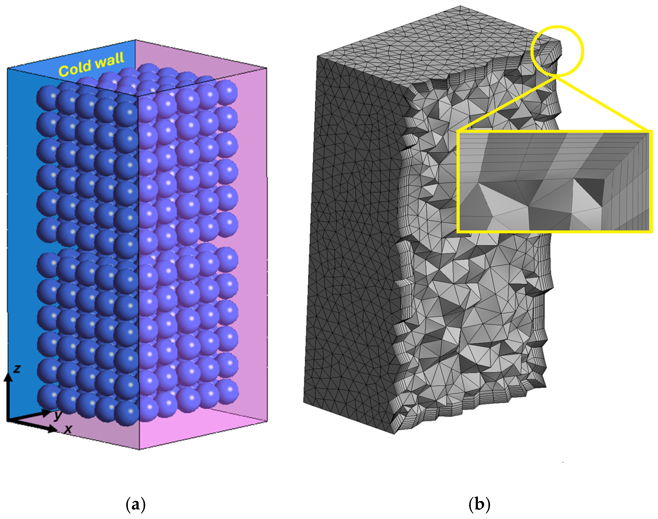
Figure 1. Refrigerator model (a) and the detail of the mesh used in the simulations (b).
Energies 18 06280 g001
Figure 2. Wall parameters, non-dimensional velocity and distance to the wall of the simulations and the representation of the log-law.
Energies 18 06280 g002
Figure 3. Horizontal temperature profile over three heights on the symmetry plane for case 0-N, and the location of the last five thermocouples in a top-view drawing.
Energies 18 06280 g003
Figure 4. (a) Air temperature near the cold wall for case 0-N. (b) Thermal and velocity profiles expected to occur in the wall region in natural convection. Note: (b) is schematic displayed here for illustrating purposes only.
Energies 18 06280 g004
Figure 5. Calculated and measured vertical air temperature profiles in case 0-N for thermocouple columns TC1 (a); TC2 (b); and TC3 (c).
Energies 18 06280 g005
Figure 6. Calculated temperature contours for case 0-N of (a) air at a plane of y = 250 mm and (b) a side wall at y = 0.
Energies 18 06280 g006
Figure 7. Calculated velocity vectors for case 0-N at a plane of y = 250 mm.
Energies 18 06280 g007
Figure 8. Calculated and measured vertical air temperature profiles in case −10-N for thermocouple columns TC1 (a); TC2 (b); and TC3 (c).
Energies 18 06280 g008
Figure 9. Calculated temperature contours for the case −10-N of (a) air at a plane of y = 250 mm and (b) a side wall at y = 0.
Energies 18 06280 g009
Figure 10. Calculated velocity vectors for the case −10-N at a plane of y = 250 mm.
Energies 18 06280 g010
Figure 11. Calculated and measured vertical air temperature profiles in case 0-Y for thermocouple columns TC1 (a); TC2 (b); and TC3 (c).
Energies 18 06280 g011
Figure 12. Calculated temperature contours for case 0-Y of (a) air at a plane of y = 250 mm, (b) air at a plane of y = 130 mm and (c) a side wall at y = 0.
Energies 18 06280 g012
Figure 13. Calculated velocity vectors for case 0-Y of (a) air at a plane of y = 250 mm and (b) air at a plane of y = 130 mm.
Energies 18 06280 g013
Figure 14. Calculated velocity vectors for cases 0-N (a), −10-N (b) and 0-Y (c) at a plane of y = 250 mm.
Energies 18 06280 g014
Table 1. Summary of cases tested and specification of each test.
Case CodeCold Wall TemperatureExistence of Spheres Inside
the Model?
Case 0-N0 °CNo
Case −10-N−10 °CNo
Case 0-Y0 °CYes
Table 2. Dimensions of the model and the locations of the thermocouples.
DimensionsTC Column 1TC Column 2TC Column 3TC Row 4TC Row 5TC Row 6Plane 1
x0–50072524355;10;15;20;25;30;35;40;45;150;300;400;450;500-
y0–500127127127250250250y = 250
z0–10002;17;34;50;66;83;97100500900-
Dimensions are in mm. TC stands for thermocouple.
Table 3. List of boundary conditions assigned to each surface of the model for the momentum equation.
ZoneCase 0-N/Case −10-N/Case 0-Y
Cold wallNWT/NWT/NWT
Side wallsNWT/NWT/NWT
Top and bottom wallsNWT/NWT/NWT
Spheresn.a./n.a./NWT
NWT—Near wall treatment. n.a.—not applicable.
Table 4. List of boundary conditions assigned to each surface of the model for the energy equation.
ZoneCase 0-N/Case −10-N/Case 0-Y
Cold wallPrescribed wall temperature + convection + radiation/Prescribed wall temperature + convection + radiation/Prescribed wall temperature + convection + radiation
Side wallsConvection + radiation/Convection + radiation/Convection + radiation
Top and bottom wallsConvection + radiation/Convection + radiation/Convection + radiation
SpheresAdiabatic/Adiabatic/Adiabatic
Table 5. Specifications of the walls employed on the model.
Wall TypeMaterialHeat Transfer Coefficient (Outer Surface) [W/m2 °C]Emissivity
(Inner Surface)
Emissivity
(Outer Surface)
Thermal Conductivity [W/m °C]
Side wallsXPS + Glass3.50.850.80.09
Top and bottom wallXPS + PVC2.50.900.80.08
Cold wallAluminum + XPSCalculated0.310.80.07
Table 6. Predicted air area-weighted average temperature for four grid sizes. Results were evaluated at a mid-plane of x = 250 mm. TAWA stands for temperature area-weighted average and ΔTAWA for the difference with the finest mesh TAWA.
Number of ElementsElement Max Size [m]TAWA [°C]
CFDExperimentalΔTAWA [°C]
181,4420.027.828.010
72,7340.037.81−0.01
55,4560.047.75−0.07
24,2540.067.64−0.18
Table 7. Convection and radiation heat transfer parameters of each case simulated, obtained from expressions in the literature and predicted using CFD calculations.
Case 0-N
Author(s)/methodRaNuHeat transfer coefficient
[W/(m2 °C)]
Heat flux rate [W]Reference temperature [°C]
Conv.Rad.Conv.Rad.Conv.Rad.
ConvectionIncropera and Dewitt [32]5.16 × 108782.2-9.1-8.2-
Vertical flat plates5.16 × 108892.5-10.2-8.2-
Çengel [26]5.16 × 1081002.8-11.5-8.2-
Qiu et al. [33]5.16 × 108561.6-6.5-8.2-
Hasanuzzaman et al. [34]n.a.331.3-5.3-8.2-
ASHRAE [35]n.a.n.a.1.6-14.2 (a)-8.2-
CFD predictionn.a.n.a.3.2-13.1-8.2-
RadiationLaguerre and Flick [1]n.a.n.a.-4.2-22.9-11.2
Tosun [36]n.a.n.a.-4.4-24.2-11.2
Acikgoz and Kincay [37]n.a.n.a.-4.3-23.7-11.2
CFD predictionn.a.n.a.-3.8-21.2-11.2
Case −10-N
Author(s)/methodRaNuHeat transfer coefficient
[W/(m2 °C)]
Heat flux rate [W]Reference temperature [°C]
Conv.Rad.Conv.Rad.Conv.Rad.
ConvectionIncropera and Dewitt [32]7.43 × 108862.4-14.1-1.8-
Vertical flat plates7.43 × 108972.7-16.1-1.8-
Çengel [26]7.43 × 1081113.1-18.4-1.8-
Qiu et al. [33]7.43 × 108631.8-10.3-1.8-
Hasanuzzaman et al. [34]n.a.331.3-7.7-1.8-
ASHRAE [35]n.a.n.a.1.6-21.8 (a)-1.8-
CFD predictionn.a.n.a.4.2-25.1-1.8-
RadiationLaguerre and Flick [1]n.a.n.a.-3.8-26.5-5.4
Tosun [36]n.a.n.a.-4.1-28.1-5.4
Acikgoz and Kincay [37]n.a.n.a.-4.3-29.8-5.4
CFD predictionn.a.n.a.-3.8-29.4-5.4
Case 0-Y
Author(s)/methodRaNuHeat transfer coefficient
[W/(m2 °C)]
Heat flux rate [W]Reference temperature [°C]
Conv.Rad.Conv.Rad.Conv.Rad.
ConvectionIncropera and Dewitt [32]4.91 × 108772.2-8.4-7.8-
Vertical flat plates4.91 × 108882.5-9.6-7.8-
Çengel [26]4.91 × 108982.8-10.7-7.8-
Qiu et al. [33]4.91 × 108551.6-6.0-7.8-
Hasanuzzaman et al. [34]n.a.331.3-5.1-7.8-
ASHRAE [35]n.a.n.a.1.6-9.76 (a)-7.8-
CFD predictionn.a.n.a.5.7-22.4-7.8-
RadiationLaguerre and Flick [1]n.a.n.a.-4.4-22.9-11.5
Tosun [36]n.a.n.a.-4.4-22.9-11.5
Acikgoz and Kincay [37]n.a.n.a.-4.3-22.2-11.5
CFD predictionn.a.n.a.-3.1-17.8-11.5
(a) This figure accounts for the heat gains through the walls, floor and ceiling of the refrigerator. n.a. stands for not applicable.
Table 8. Summary of the main characteristics of the software packages considered.
SoftwareMain ApplicationType of CalculationLevel of DetailEquipment SelectionCostAdditional Notes
HVACR WICFWalk-in coolers and freezers (small and medium cold rooms)Total heat load (transmission, infiltration, product)Basic to intermediateYes, based on generic dataUsually paidComplies with DOE (USA) standards; recommended for quick design of cold rooms.
KR LoadCalcCold rooms and refrigerated warehousesTotal heat loadBasicYes, linked to KeepRite productsFree (with registration)Aimed at contractors; limited to the brand’s equipment portfolio.
Intarcon Client360Commercial and industrial refrigeration systemsTotal heat load + system optimizationIntermediate to advancedYes, within Intarcon’s portfolioFree (for clients)User-friendly interface; integrated with European regulations.
Table 9. Comparison of the selected input variables by software.
ParametersHVACR WICFKR LoadCalcIntarcon
Floor typeOn-gradeOn-gradeOn-grade
Exterior temperature (°C)202020
Indoor temperature (°C)8.28.28.2
Insulation thermal conductivity [W/m °C]0.07 to 0.090.07 to 0.090.07 to 0.09
Product weight (kg/24 h)n.a.n.a.n.a.
Internal load (W)000
Operation time (h)181818
Table 10. Comparison of evaporator cooling capacity estimated by the selected software and calculated using the CFD model for Case 0-N.
Software/MethodHVACR WICFKR LoadCalcIntarconCFD
Heat flux rate [W]26.011.022.634.3
Percentage difference [%]24.5102.941.10
Disclaimer/Publisher’s Note: The statements, opinions and data contained in all publications are solely those of the individual author(s) and contributor(s) and not of MDPI and/or the editor(s). MDPI and/or the editor(s) disclaim responsibility for any injury to people or property resulting from any ideas, methods, instructions or products referred to in the content.