Article

Influence of Surface Complexity and Atmospheric Stability on Wind Shear and Turbulence in a Peri-Urban Wind Energy Site

1
National Wind Institute, Civil, Environmental and Construction Engineering, Texas Tech University, Lubbock, TX 79409, USA
2
Department of Mathematics, Texas Tech University, Lubbock, TX 79409, USA
3
IIHR-Hydroscience and Engineering, The University of Iowa, Iowa City, IA 52242, USA
4
Civil and Environmental Engineering, The University of Iowa, Iowa City, IA 52242, USA
*
Author to whom correspondence should be addressed.
Energies 2025, 18(19), 5211; https://doi.org/10.3390/en18195211
Submission received: 4 August 2025 / Revised: 12 September 2025 / Accepted: 19 September 2025 / Published: 30 September 2025

Abstract

The large-scale deployment of wind energy underscores the critical need for accurate resource characterization to reduce uncertainty in power estimates and to enable the installation of wind farms in increasingly complex terrains. Accurate wind resource assessment in peri-urban and moderately complex terrains remains a significant challenge due to spatial heterogeneity in surface terrain features and atmospheric thermal stability. This study investigates the influence of surface complexity and atmospheric stratification on vertical wind profiles at a utility-scale wind turbine site in Cedar Rapids, Iowa. One year of multi-level wind data from a 106-meter-tall meteorological tower were analyzed to quantify variations in the wind shear exponent α , wind direction veer, and horizontal turbulence intensity (TI) across open-field and complex-surface wind sectors and four thermal stability classes, defined by the bulk Richardson number R i b . The results show that the wind shear exponent α increases systematically with atmospheric stability. Over the open-field terrain, α ranges from 0.11 in unstable conditions to 0.45 in strongly stable conditions, compared to 0.17 and 0.40 over the complex surface. A pronounced diurnal variation in α was observed, particularly during the summer months. Wind veer was greatest and exceeded 30° under strongly stable conditions over open terrain. Elevated TI values peaked at 32 m in height due to flow separation and wake turbulence from nearby vegetation and sloping terrain. These findings highlight the importance of incorporating terrain-induced and thermally driven variability into wind resource assessments to improve power prediction and turbine siting in complex heterogeneous terrain environments.

1. Introduction

As a key driver in the global energy transition, wind energy plays a crucial role in reducing reliance on fossil fuels and meeting decarbonization targets. Projections suggest that between 70% and 90% of new renewable energy development will come from wind and solar sources [1,2,3]. The large-scale deployment of wind energy highlights the need for reliable wind resource characterization, since accurately representing wind conditions reduces uncertainty in power production forecasts and improves both the efficiency and cost-effectiveness of energy system integration [4,5]. As deployment accelerates, wind turbines and wind farms are increasingly being installed in more complex terrains—extending beyond flat, homogeneous landscapes to regions characterized by hills, escarpments, slopes, vegetation, water bodies, and scattered surface obstacles [6,7,8,9,10]. These complex settings present significant challenges for accurately predicting wind speed, wind direction, and turbulence, which are critical for wind resource assessment and turbine performance evaluation. Even in moderately complex inland environments—such as semi-open areas near urban boundaries—accurate modeling of wind profiles remains difficult. In such settings, the atmospheric boundary layer (ABL) is highly dynamic, continually responding to surface heterogeneity, generating turbulent wakes, and forming internal boundary layers, often without achieving equilibrium. Despite these complexities, there remains a lack of widely accepted analytical models capable of capturing atmospheric boundary layer (ABL) wind dynamics under non-equilibrium conditions [11]. In parallel with these challenges, wind turbine design continues to evolve.
Wind turbine hub heights have increased significantly in recent decades, both onshore and offshore. According to the International Energy Agency (IEA) Wind TCP Task 26 report [12], the average onshore hub height in Germany rose from 101 m in 2010 to 141 m in 2018, with tip heights now frequently exceeding 200 m. Offshore installations have followed a similar trajectory, with average hub heights increasing from approximately 83 m in 2010 to 108 m by 2019. Reflecting the trend toward larger machines, the GE Haliade-X turbine features a hub height of 156 m and a tip height of 276 m [13]. As turbines increase in height and rotor-swept area, atmospheric thermal stability—driven by diurnal heating and cooling—becomes an increasingly influential factor in turbine performance. This trend underscores the growing importance of accurately representing both surface complexity and atmospheric stability, further complicating wind resource assessment. Variation in surface features and atmospheric stability introduces substantial spatial and temporal variability in wind fields, which remains a leading source of uncertainty in the wind energy sector. Even small errors—on the order of 1 m/s in mean wind speed estimates—can result in millions of dollars in annual revenue losses for utility-scale wind farms [4]. While wind resource assessments typically emphasize mean wind speed and air density, other atmospheric parameters—such as wind shear, veer, and turbulence intensity—are less frequently included in standard modeling frameworks. However, these factors can significantly influence turbine power output, contributing up to 10% variation even when wind speed and density are accurately accounted for [14]. For example, a recent study conducted at a utility-scale turbine located at Kirkwood Community College (KCC) in Cedar Rapids, Iowa, demonstrated that incorporating air density, wind shear, veer, and turbulence intensity into the wind profile model markedly improved power prediction accuracy [15].
Another critical atmospheric variable for wind turbine performance and control is wind direction. Wind direction is a critical factor in determining the design wind speed for structural loading and for enabling real-time control of wind turbines to optimize power production [7,16]. Wind direction varies significantly in space and time and must be accounted for in yaw control systems that orient the nacelle and blades toward the prevailing wind. Effective yaw alignment is particularly important in the presence of wind veer—vertical variation in wind direction—which can reduce power output and increase asymmetric loading on turbine blades [17,18]. Advanced turbine control strategies are increasingly designed to mitigate the effects of wind shear, veer, and turbulence, especially under unstable atmospheric conditions [15,19]. In complex terrains composed of significant surface topography (hills/mountains, escarpments, ridges, valleys, forests, or abrupt surface changes), flow unsteadiness and elevated turbulence intensities significantly increase structural loading and fatigue, resulting in increased maintenance and reducing turbine lifespan [7,16]. These effects underscore the importance of accurate modeling and prediction of local turbulent wind fields, particularly over heterogeneous surfaces and topography [20]. Reliable simulations and measurements of these wind fields are essential for wind resource assessment, optimizing wind turbine micro-siting, and informing the design and operation of control systems in modern wind energy projects [19].
Due to the high costs associated with tall meteorological masts and ground-based Lidar systems, wind measurements are often limited to heights below those most relevant for wind turbine operation. In many regions, wind data are most readily available at a standard height of 10 m, such as those provided by Mesonet stations. Consequently, reliable and robust extrapolation models are essential for accurately predicting wind conditions at turbine-relevant heights and for enabling effective turbine control. However, this reliance on extrapolation introduces challenges to wind resource assessment, as critical parameters—such as wind speed, direction, and turbulence—must be estimated at heights spanning the rotor-swept area, often well above the available measurements. To estimate winds at operational heights, measurements are commonly taken at two or three levels—e.g., 2 m, 6 m, and 10 m using a met tower. These near-surface data are then used in extrapolation techniques, such as power-law or logarithmic wind profiles, to estimate wind speeds at greater heights. However, the accuracy of these methods can be significantly influenced by atmospheric stability, surface complexity, and the availability of vertical profile data. It remains an open question whether wind and turbulence information at the rotor plane can be obtained via extrapolation from near-ground measurements. Previous research suggests that specific prediction models should be developed for a site [21,22], ideally based on wind data measured at multiple heights.
Over homogeneous rough surfaces and under neutral stratification conditions, the logarithmic wind profile—derived from fundamental turbulence scaling theory—relates the vertical gradient of wind speed to the friction velocity u * , the von Karman constant κ , and the height above the surface z. Upon integration, the mean wind speed profile U ( z ) becomes a logarithmic function of the height, the aerodynamic roughness length z 0 , and u * . This formulation serves as the foundation for many wind profile extrapolation methods in neutral stability conditions. To account for the effects of thermal stability on the shape of wind profiles, Monin–Obukhov Similarity Theory (MOST) introduces a stability correction with a function ψ m ( z / L ), where L is the Obukhov length. Under stable or unstable stratification, this correction modifies the shape of the logarithmic wind profile to reflect the influence of buoyancy on turbulent mixing [23,24]:
U z = u * κ ln z z d z 0 ψ m z L .
MOST is applicable for representing wind profiles within the surface layer of the ABL, approximately the lowest 10% or up to about 100 m above the ground level. For winds over clusters of buildings and trees forming a so-called urban canopy, the zero-plane displacement height z d is used to account for the fact that the logarithmic law is shifted upwards due to the roughness sub-layer (RSL). Even for a steady, fully-developed turbulent wind flow of neutral stability, determining these three parameters z 0 , z d , and u * based on a best fit to field measurements can introduce large uncertainties [25,26]. Alternatively, the empirical power law is commonly used in wind engineering applications to define vertical wind profiles [27] and for resource assessment of wind energy (see International Electrotechnical Commission (IEC) standards: (IEC61400-1, 2019, IEC61400-2, 2013) [28,29]):
U ( z ) U ( z r e f ) = z z r e f α ,
where z r e f is the reference height, U ( z r e f ) is the mean wind speed at the reference height, and α is the power-law exponent or the wind shear exponent. In fact, the log-law and power-law models can be related by setting the vertical gradient forms equal at a given height z for neutral stability conditions, resulting in a relationship α = ln [ z z r e f ] . The advantage of the power-law model is that it only requires determining one parameter, the exponent α for the wind profile.
The power-law exponent of 1/7 is well established for turbulent boundary layer winds over flat, horizontally homogeneous surfaces. However, it has been found to typically vary from 0.1 over a smooth surface ( z 0 = 0.001 m) to 0.4 over rough surfaces ( z 0 = 3 m) [30]. Using these values often assumes a reference height of 10 m above the ground level, which is the international standard height for weather stations. Note, however, that the value of the shear exponent α is dependent on the specific height of the reference measurement and therefore should be interpreted carefully. As the RSL of the urban canopy is three to five times the height of buildings and trees, reference measurements made within the RSL can lead to significant errors. Drew et al. [31] and Lange et al. [32] demonstrated that wind prediction methods that assume uniformly flat terrain can result in an error of up to 20% when applied to complex heterogeneous terrain.
With the trend toward larger turbines, the wind energy community has investigated how atmospheric stability influences the shear exponent α [33,34,35]. Several studies have reported its dependence on atmospheric stability over flat, open-terrain sites. For example, Newman and Klein [35] investigated α values for different stability regimes at the Cheyenne Mesonet site in August 2009. The 10 m and 80 m wind speed data measured by cup anemometers from a nearby tall tower were used to obtain the shear exponent α . Gualtieri [36] studied power-law mean wind profiles using the 10 min averaged data of three years by a met mast at Cabauw, Netherlands. The site is characterized as flat with an estimated roughness length of 0.02 m. Gualtieri [37] examined the dependence of α on Pasquill classes of thermal stability. The results show that whereas α (of 0.2) does not vary significantly for unstable cases of various strengths, it monotonically increases from 0.2 to 0.47 for the neutral and stable cases.
Fewer studies of the shear exponent α have been reported over moderately complex peri-urban sites, like the site of Cedar Rapids, Iowa, where we have access to comprehensive datasets at a multi-level met tower for a duration of a year. These data provide an excellent opportunity to address the effects of the atmospheric thermal stability on wind profiles (via the power-law shear exponent α and wind direction) and turbulence intensity for a realistic site of moderately complex surface landscapes. Therefore, the objectives of this research are as follows: (1) to characterize the mean wind speed and direction at several elevations corresponding to two distinct surface features—open field and more complex surface; (2) to examine the range and statistical characteristics of the wind shear exponent α to clarify the effects of the thermal stability coupled with the moderately complex surface landscapes; and (3) to determine the horizontal turbulence intensities and understand the wind flow regimes over heterogeneous surfaces under atmospheric thermal stability conditions. This study is a continuation of our earlier work, with preliminary analysis presented in Ahlman et al. [38]. The results will clarify the effect of atmospheric thermal stability and heterogeneous surface features on wind field characteristics and improve the prediction of wind profiles at wind-turbine relevant heights from the measurements at lower levels.

2. Data Acquisition and Analysis Methodology

2.1. Field Site, Equipment, and Data Collection

A year of data, used in this study, were collected on a 106 m tall telecommunications tower on the campus of Kirkwood Community College in southwest Cedar Rapids, Iowa (latitude, 41 ° 54 33 N; longitude, 91 ° 39 18 W). The tower was instrumented with meteorological sensors at six heights (met tower). The data were collected from September 2017 to September 2018. A 2.5-MW Clipper Liberty C96 turbine is located approximately 900 m NNE of the tower, with the Cedar Rapids urban core 8 km to the north and rural land directly to the south and east. As shown in Figure 1, the spatial distribution of civil structures exhibits heterogeneous features. In the NW direction, the urban canopy is characterized by a forest of trees beginning roughly 200 m upwind of the tower. Beyond that, low-density residential housing of one- and two-story homes appears around 400 m upwind, followed by a city block of three-story apartments at about 600 m (see 2D transect of topography in Figure 2). The forest trees are primarily deciduous trees between 15 and 20 m tall, which would be considered aerodynamically dense with a nominal displacement height Z d between 70% and 80% of the total height [23].
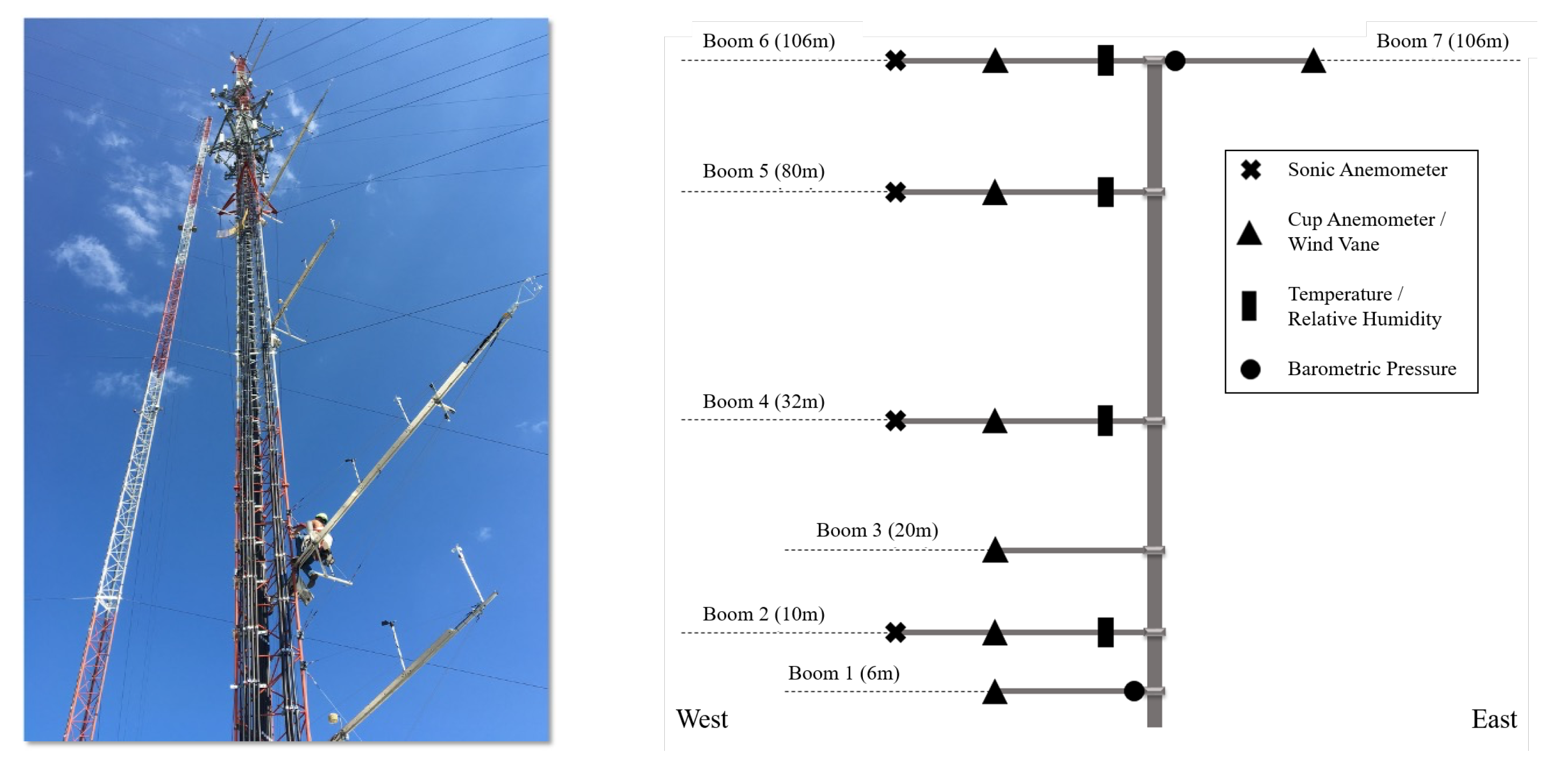
The meteorological tower is instrumented with cup and sonic anemometers, barometers, and temperature and relative humidity sensors, as summarized in Table 1. A schematic of the tower and sensor arrangement is shown in Figure 3, with icons indicating the instruments mounted on each of the seven booms. Booms 1–6 extend westward, while Boom 7 extends eastward. Boom 4 ( Z = 32 m) aligns with the lower tip of the nearby wind turbine rotor, Boom 5 ( Z = 80 m) corresponds to hub height, and Booms 6 and 7 ( Z = 106 m) are positioned at the top of the tower. Sonic anemometers are installed on Booms 2, 4, 5, and 6, and were operated during specific periods for the studies on how different levels of turbulence affect wind turbine performance in [15,20]. To minimize tower interference, these booms are 6.4 m (21 ft) long, compared to 3.66 m (12 ft) for the others. The cup anemometers used are A100LK models from Campbell Scientific (Logan, UT, USA), and the wind vanes are NRG 200P models from NRG Systems (Hinesburg, VT, USA). According to the NRG 200P specifications, potentiometer linearity is within 1%. The wind vanes meet IEC 61400-12-1 Sec. 6.3 standards [39], and the combined uncertainty in calibration, operation, and orientation for wind direction measurements is less than 5°. Data from the cup anemometers, temperature sensors, wind vanes, and pressure sensors are used primarily to characterize boundary-layer winds in this study.

2.2. Data Quality Assessment

Field measurements of the atmospheric boundary layer (ABL) are inherently complex due to the dynamic nature of atmospheric processes, making data analysis a nontrivial task. Furthermore, data collection can be interrupted by sensor malfunctions or unforeseen environmental influences, such as heavy precipitation and icing conditions, introducing uncertainty. Therefore, a rigorous data quality assessment is essential prior to any analysis. In this study, several measures were implemented to evaluate the quality of the 1-year data set. These included evaluating data completeness at each boom level, verifying consistency with meteorological observations from the nearby weather station at Cedar Rapids Airport (CID, ASOS), and examining potential tower shadowing effects on wind speed measurements. All sensors were new and calibrated by the manufacturer just prior to deployment.
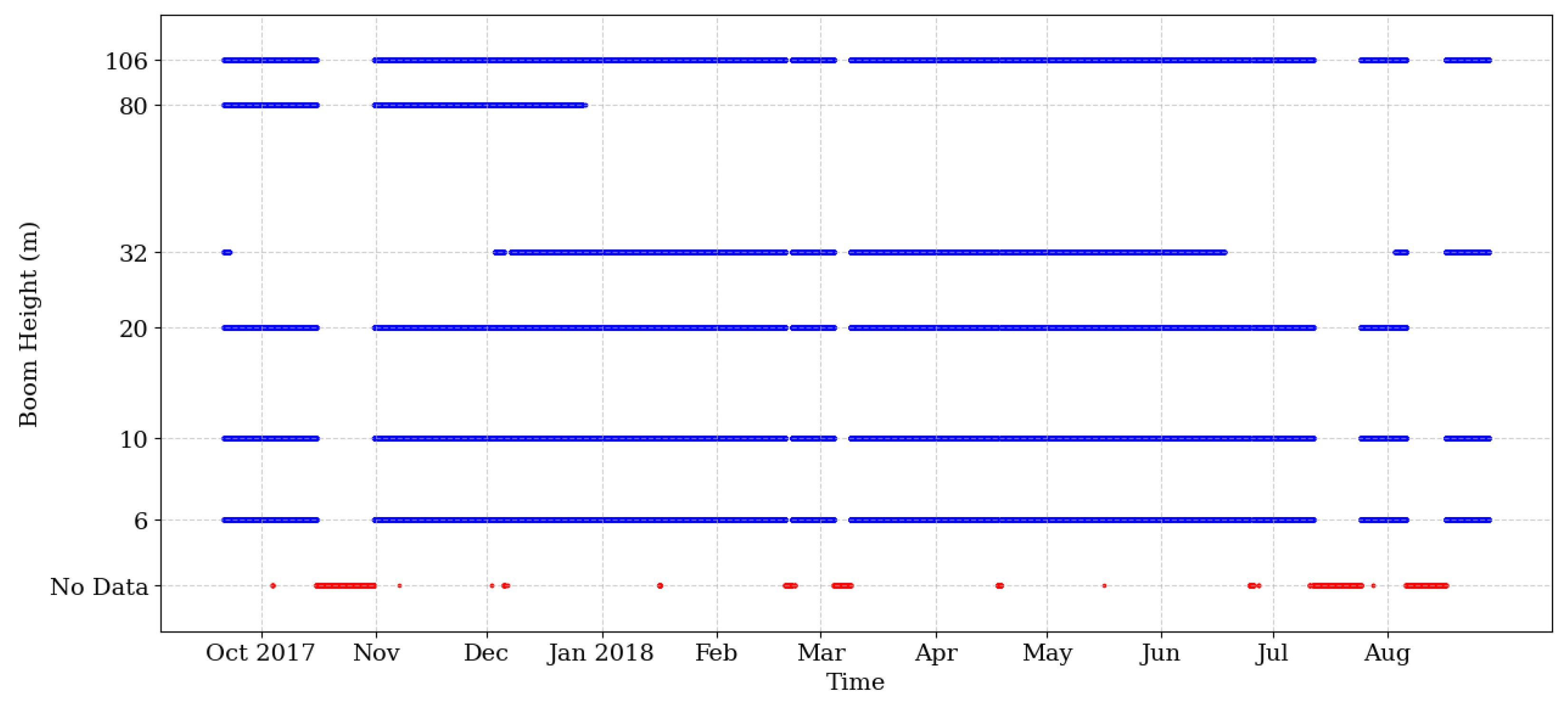
The data collected by each sensor was first assessed for completeness and continuity in various inspection periods. This revealed that a large part of the data was missing from Boom 5 ( Z = 80 m), which did not record after the end of 2017 due to interference, from a newly installed radio communication antenna, with data transfer (Figure 4). As a result, the Boom 5 data were excluded from the analysis. In addition, there are brief gaps in the data at all booms due to periods of tower maintenance. Otherwise, the data are complete from the cup anemometers, wind vanes, and temperature sensors mounted on all the other booms. Subsequently, outliers were identified as data that deviated by more than five standard deviations from a 30-min running mean, and these were removed, following Vahidzadeh and Markfort [15]. The outlier removal procedure resulted in the elimination of approximately 0.01% of the total data. The data were then resampled from their original 1-min intervals into 10-min averaged points. Care was taken to ensure that wind vectors were averaged using true (i.e., rectangular form) vector averaging, for maximum accuracy in the resampled data. Furthermore, since the bulk Richardson number calculations require data at 6, 10, and 106 m, data missing at timestamps for any of these were excluded from the analysis. After resampling and removal of incomplete data, there were 42,740 data points in 10-min increments, which is equivalent to 296 total days of coverage. The time periods of the remaining data after the quality control steps are shown in Figure 4. All the data shown were used in the analysis, except for the incomplete data from Boom 5 at Z = 80 m.
The direction of the wind varies both in time and in space. To minimize shadowing effects on the data, the booms and sensor mounting were designed in accordance with IEC 61400-12 guidelines, ensuring that the sensors were spaced approximately 6.5 tower diameters apart. As shown in Figure 3, Booms 6 and 7 are oriented in opposite directions on top of the met tower ( Z = 106 m). The wind speed recorded from the cup anemometers at booms 6 and 7 was compared to assess any potential impact from shadowing. It was observed that when winds were blowing within 15° of due east (90°) or west (270°), there were clear discrepancies between the measurements of the two booms. This is due to Boom 6, located on the west side of the tower, experiencing shadowing when the wind blows from the east, and Boom 7 experiencing similar effects when the wind comes from the west. To resolve this issue, when one boom was deemed shadowed (i.e., the wind direction was within 15° of its shadowing direction), the wind speed and direction of the unshadowed boom were taken as representative values at 106 m; otherwise, when neither boom was shadowed, the vector-average wind reading between the two measurements was used. It is important to note that this shadowing-merge procedure does not affect the subsequent analyses presented in this text, since the open-field and complex-surface sectors defined in Section 2.3 do not overlap with these shadowing zones. Therefore, for the remainder of this document, a simple vector averaging between the two booms may be assumed.
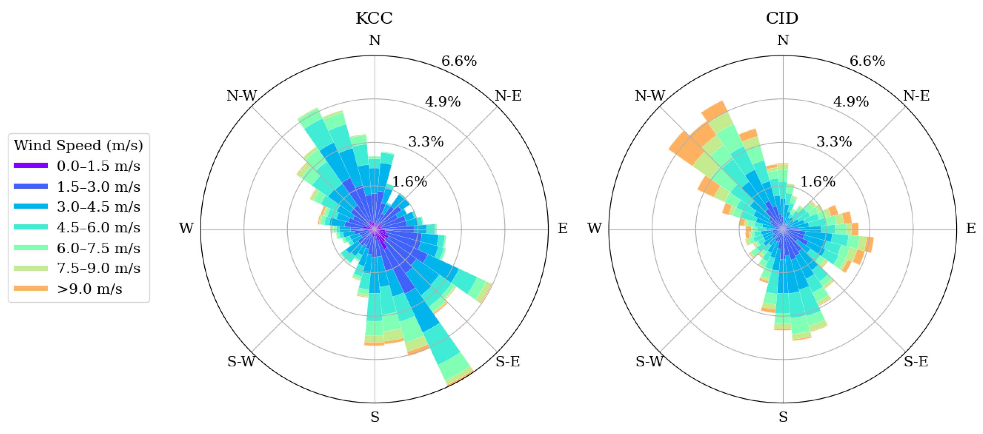
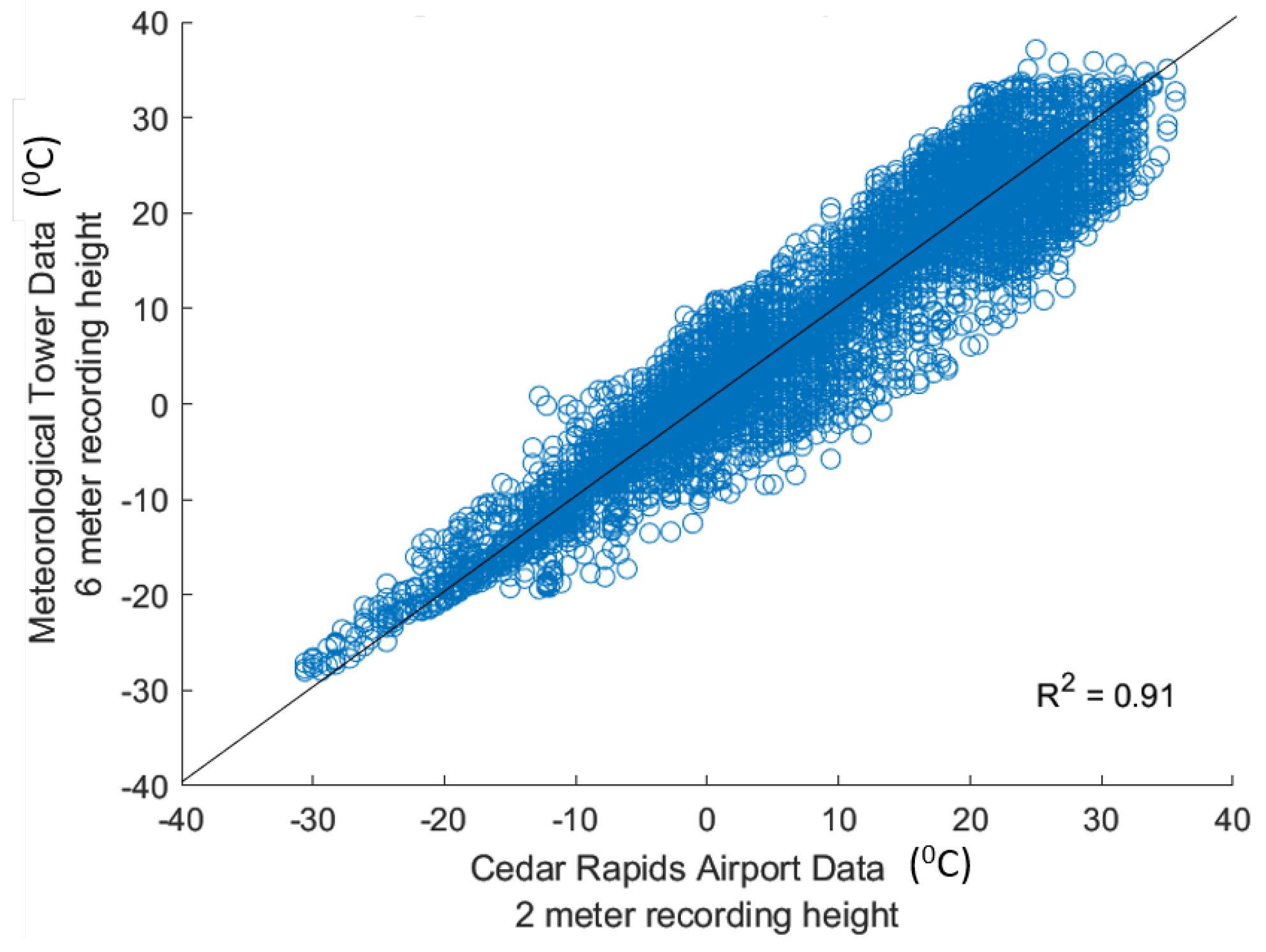
Wind direction and temperature data recorded at the Cedar Rapids Airport (CID) weather station, located 6.46 km (4.01 miles) southwest of the 106 m met tower, were acquired from the Iowa Environmental Mesonet (IEM) to evaluate the consistency of the data between the two sites. Wind roses were generated using measurements of wind speed and direction from Boom 2 ( Z = 10 m) on the met tower, and from the same 10 m height at CID (Figure 5). In both cases, the dominant wind directions were from the northwest and the southeast, consistent with typical seasonal patterns in the Midwestern United States—northwesterly winds during winter and southeasterly during summer. While the wind direction patterns were similar between the two sites, the wind speed magnitudes differed, likely due to variations in surface roughness and local terrain characteristics. The airport is located in a relatively open environment, whereas the meteorological tower is located in a peri-urban area with nearby buildings and urban forests, which likely induce greater flow disruption and attenuation. Furthermore, the near-surface air temperatures recorded at Boom 1 ( Z = 6 m) on the met tower were compared with those recorded at 2 m above ground level at CID (Figure 6). The comparison demonstrates strong agreement, with a correlation coefficient of R 2 = 0.91 , indicating reliable consistency in temperature measurements between the two sites. In general, the wind and temperature measurements from the meteorological tower are consistent with those obtained from the airport weather station, providing additional confidence in the tower data for the subsequent analysis.

2.3. Classification of Terrain Features and Atmospheric Thermal Stability

In analyzing wind data acquired from a met tower, which inherently reflect the combined effects of various environmental factors, a common strategy is to first identify relatively clean conditions and then categorize the data based on dominant influences. The vertical structure of the ABL is primarily influenced by terrain and surface roughness characteristics, along with atmospheric thermal stability. While civil structures (e.g., buildings) remain relatively constant year-round, vegetation such as trees and crops shows marked seasonal variability. To account for these influences, met tower data are often analyzed in 30°- or 60°-directional sectors to assess terrain and roughness effects. The predominant wind directions are observed to be from the northwest (285°–345°) and southeast (105°–165°), as shown by the wind rose (Figure 5). In addition, the surface features of the northwest and southeast wind sectors are distinctly different. The northwest sector is characterized by clusters of one- and two-story residential buildings having a dense tree canopy, while the southeast sector is characterized by a relatively open agricultural area, with a few scattered low-rise buildings several hundred meters from the met tower. The alignment of different surface features with predominant wind directions suggests that wind data can be categorized into “open-field” and “complex-surface” sectors. Specifically, by including only wind data from the northwest direction (285°–345°), we can focus on the wind profiles developed over the surface of greater heterogeneity. Wind profiles over a relatively open field are constructed from wind data of the southeast direction (105°–165°). After this final step of filtering the data set for wind direction, brief periods of heavy precipitation and snow/ice conditions were also removed. After quality control and filtering for wind sectors, the final data set was reduced to 42,265, or about 98.9% of the original data collected (see Figure 4).
Researchers have used different measures and criteria to classify atmospheric thermal stability, creating challenges when comparing results between studies and implementing wind speed extrapolation schemes [40]. For example, Pasquill atmospheric stability classes are based on surface wind speed, temperature change, daytime insulation, and nighttime overcast conditions, which need engineering judgment when assigning a specific stability class. The gradient Richardson number and the bulk Richardson number R i b can be estimated to classify the thermal stability strength using data collected at different heights [21,35,37]. In this study, we used R i b based on the data collected for temperature, humidity, and pressure, as well as cup anemometers and wind vanes. The bulk Richardson number is preferred because it measures the ratio of buoyancy-associated effects on turbulence to shear-generated turbulence. Negative values of R i b indicate stronger vertical mixing due to surface heating, values near zero indicate entirely shear-driven turbulence, and positive values indicate suppression of turbulence due to stratification. The bulk Richardson number R i b was calculated for 10-min averaged periods using the following expression:
R i b = g Δ θ v ¯ Δ z θ v ¯ [ ( Δ U ¯ ) 2 + ( Δ V ¯ ) 2 ] ,
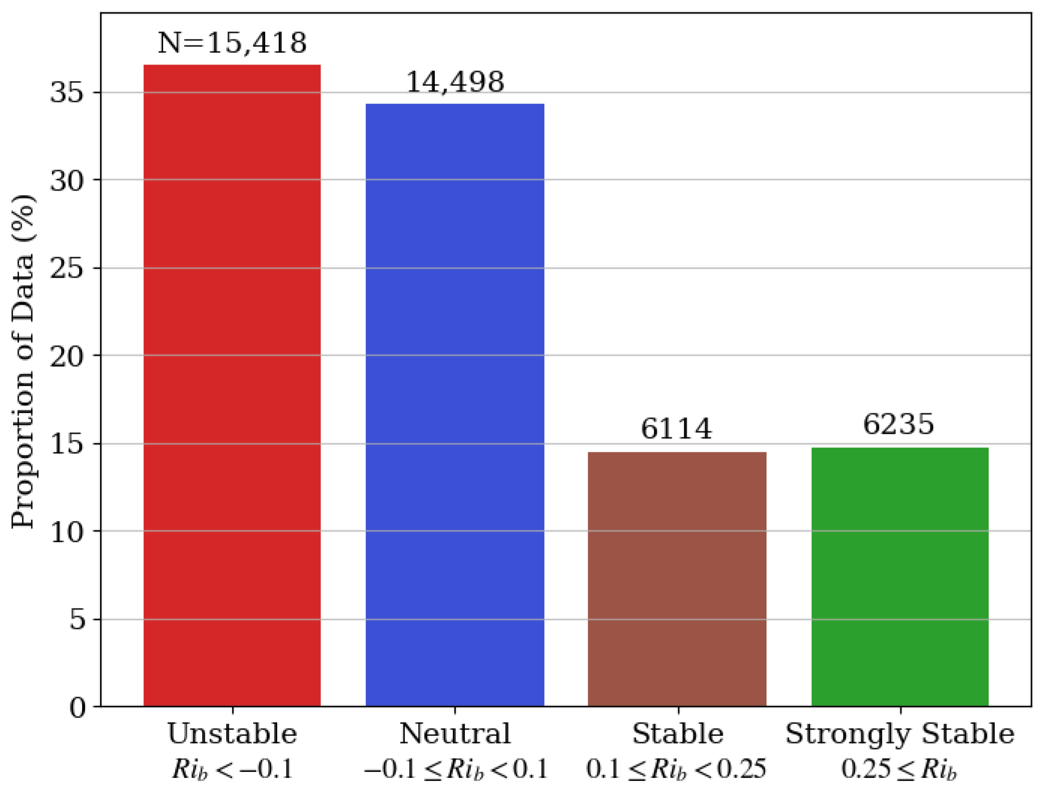
where θ v is the virtual potential temperature, Δ z is the difference in measurement heights, g is gravitational acceleration, and U and V are the horizontal velocity components of the wind, respectively [24]. Overbars on variables indicate time averaging. Data from Boom 6 ( Z = 106 m) and Boom 2 ( Z = 10 m) were used to calculate the Richardson number. Among all booms, Booms 2 and 6 provided the most comprehensive and reliable data. Compared to Boom 1, the data from Boom 2 were used because the measurements were less variable, presumably due to the closer proximity of Boom 1 to the ground. Various classification criteria have been proposed in prior research, using three to five categories of stability. In this study, classification of thermal stability was determined based on the specific ranges proposed in [35,41]. Specifically, atmospheric stability is classified into four categories: Unstable ( R i b < 0.1 ), Neutral ( 0.1 R i b < 0.1 ), Stable ( 0.1 R i b < 0.25 ), and Strongly Stable ( R i b 0.25 ). Following this classification, the wind data for the entire year were segmented as shown in Figure 7. The Unstable cases account for approximately 37% of the total data, Neutral cases for 34%, Stable cases for 14%, and Strongly Stable cases for 15%.
The virtual potential temperatures θ v at Booms 2 and 6 are needed to compute R i b in Equation (3). The data acquired at Booms 2 and 6 include the relative humidity fraction R H , temperature T (K), and barometric pressure P (kPa). Because Boom 2 ( Z = 10 m) was not equipped with a barometer, pressure readings from Boom 1 ( Z = 6 m) were used. We first compute the vapor pressure P v a p as
P v a p = R H · P s a t ( T ) ,
where P s a t is approximated using Tetens’ Equation following [42],
P s a t ( T ) ( 0.6113 kPa ) exp 17.2694 T 273.15 K T 35.86 K .
We then compute the potential temperature θ as
θ = T 100 kPa P R / C p ,
where R / C p 0.286 is the gas constant of air divided by its specific heat capacity. The water–air mixing ratio w is calculated as
w = 0.622 P v a p P P v a p ,
and finally we compute θ v by
θ v = θ 1 + w / 0.622 1 + w .

2.4. Power-Law Model of Mean Wind Profiles

As the only parameter to be determined in the power-law model, the exponent α varies with time and depends on land cover and terrain characteristics. The value of α is also affected by the specific method of analyzing the raw data. In a recent review, Gualtieri [43] summarized various ways to assess the power-law exponent α . Among them, the PL( α )- α model considers an overall yearly averaged value using data at two elevations. The PL( α )- α (t) model is based on measured overall mean α values varying by hour of day and/or month of year. The PL( α )- α s t a b model employs the measured overall mean α values sorted by stability class, i.e., stability-averaged α values. The PL( α )- α w s model uses the overall mean α values sorted by wind sectors, i.e., sector-averaged measured α values. The form of the power-law function used for the regression analysis is
U ( z ) = β z α .
The coefficient β represents the magnitude of the wind speed, while the wind shear exponent α depends on the shape of the wind profile, which is equivalent to that of Equation (2). Wind direction sectors and the bulk Richardson number serve as the primary means of segmentation for the data in this study. The power-law model was obtained by fitting the 10-min average wind speed at each height for β and α . Since the quality control confirmed that data are available at 6, 10, and 106 m, the power law fits use data from at least three heights. In over 99.9% of the time, data were also available at 20 m or 32 m, allowing for at least four and often five heights to be included in the regression. Sensitivity tests were performed, and it was found that removing portions of the data from Boom 4 did not significantly affect the results.

3. Results and Discussion

3.1. Variation of Mean Wind Speed Profiles with Height

The distributions of wind speeds at each height for the open-field and complex-surface sectors are examined in Figure 8. These were found to be described by Weibull distributions, with shape parameter k and scale parameter λ [44]. Wind speeds are generally higher and more consistent at higher altitudes, especially above 20 m. The complex-surface sector shows slightly higher mean wind speeds (higher λ values) at most heights. At the lower levels of 6 m and 10 m, wind speed distributions are more skewed towards lower magnitudes (with k less than 2) and thus wind speeds appear stronger over complex surfaces. The impacts of different surface, open field (105°–165°) or complex surface (285°–345°), on the Weibull distribution tend to decrease while moving away from the ground level.
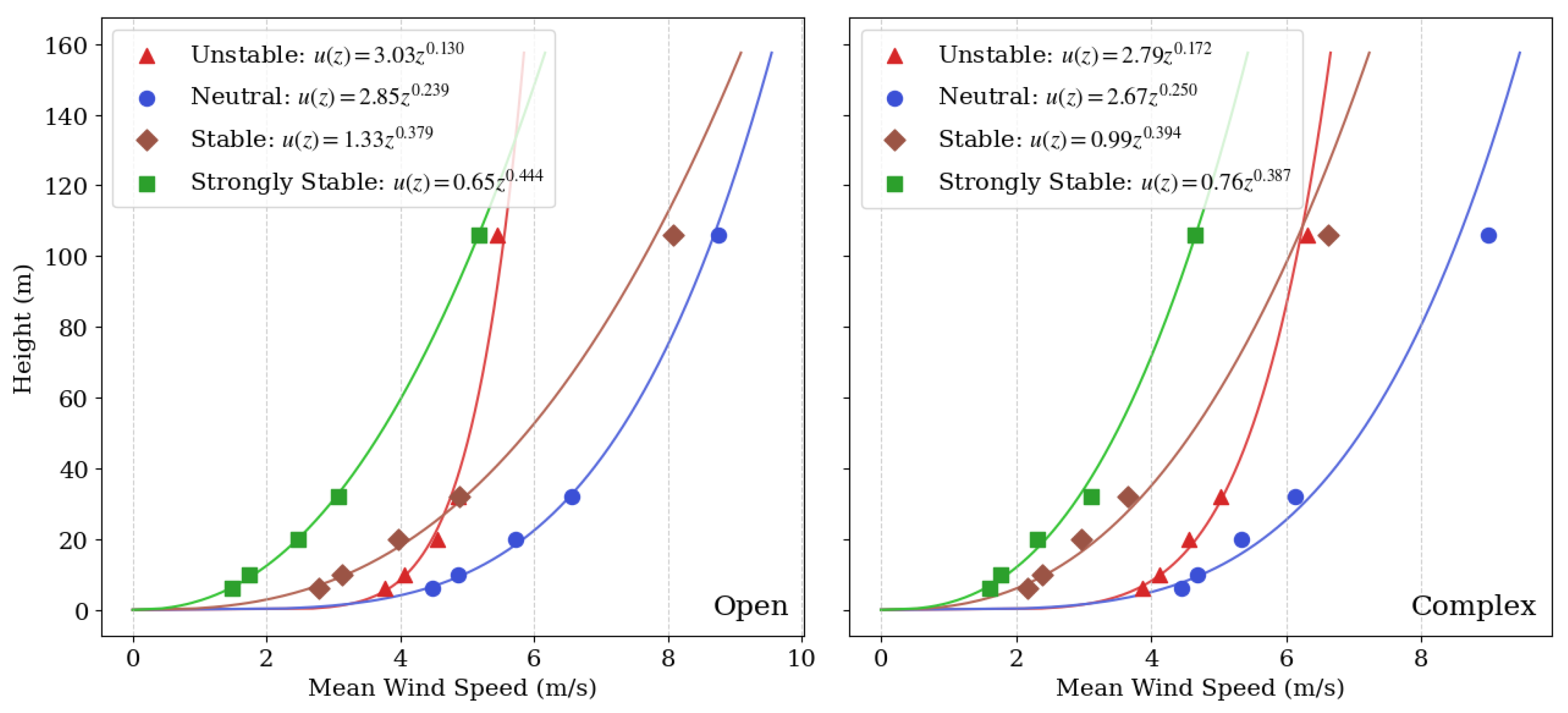
Typically, the vertical profiles of annual mean wind speeds are used to generate the power-law model. These mean wind speeds for specific cases of thermal stability and terrain are shown in Figure 9. Over the open field, and for neutral stability, the wind shear exponent α is approximately 0.24, nearly twice as large as the commonly assumed value of 1/7, based on idealized experiments. The deviation indicates that the “open-field” wind sector of the field site cannot be assumed to be an idealized horizontally homogeneous rough surface. Instead, the increased roughness is primarily due to surface heterogeneity from the agricultural landscape, scattered low-rise commercial buildings, and possibly the sparse rows of trees along the nearby roadway, and this effect should be considered significant. Interestingly, under neutral conditions, α is 0.25 for the complex surface sector, which is comparable to that for the open field.
Mean wind speeds are generally higher at all heights under neutral stability compared to stable or unstable thermal conditions. This is expected since R i b approaches zero for stronger winds and explains why wind loading standards for civil structures typically ignore atmospheric thermal stability. However, thermal stability significantly influences the shape of mean wind profiles and, consequently, the wind shear exponent α , as shown in Figure 9. The unstable case exhibits weaker shear with a lower α , while stable and strongly stable cases show stronger shear with higher α . Overall, α increases with R i b for both the open-field and complex-surface sectors at this site, except in the strongly stable class, where α is slightly lower than in the stable class.
As pointed out by Gualtieri [43], the values of the wind shear exponent α determined using different methods do not necessarily yield the same results. An alternative approach is to obtain the α of each 10 min segment of wind profiles; thus, a database of α values based on different stability classes and two terrain features is built for statistical analysis. Figure 10 illustrates the distribution of α for different thermal stability and terrain classes, similar to Sathe and Bierbooms [33]. The median and mean values of α are approximately the same, which increase as R i b increases. In the unstable and strongly stable stability cases, the median/mean values of α show a significant difference between the two terrains. It is noted that there is more variation in α values for the stable and strongly stable classes, with the standard deviation of the strongly stable case being 0.21, roughly triple that of the unstable case for the complex surface. The skewness of the α distributions also varies with thermal stability. In particular, for the unstable and strongly stable cases, the distribution shift is opposite for the open-field and complex-surface sectors.
Median and mean wind shear exponent α values corresponding to specific thermal stability and terrain features are summarized in Table 2. For a given thermal stability class and terrain feature, the values of α show consistency from two approaches. The first approach is based on an overall vertical profile of mean wind speed by 10 min segment of wind data sorted with specific thermal stability and terrain feature (Figure 9). The second approach is to obtain the α of each 10 min segment of wind profiles, and thus a database of α values based on different stability classes and two terrain features is built for statistical analysis (Figure 10). Although α is almost the same over the open-field and complex-surface sectors for the neutral, stable, and strongly stable cases, in unstable cases, α over the open field (0.12) is approximately 29% lower than that over the complex-surface sector (0.17). We compared α values over the open terrain for different stability cases with Newman and Klein [35] and Gualtieri [37]. The values of α reported in Newman and Klein [35] are noticeably less than those obtained for the open-field terrain and the neutral, stable and strongly stable cases (except the unstable case) at the Cedar Rapids, Iowa, site. Our data are aligned with the α values in Gualtieri [37] in the neutral, stable, and strongly stable cases, but are only about half of that in the unstable case. Compared with data at multiple sites in Touma [21], the α values of this study fall in the reported range and show a similar increasing trend with increasing R i b . Given the different methods of determining the stability classes and the variation of surface terrain in these works, it seems that the α values exhibit greater variation for the unstable case compared with those in the neutral or stable and strongly stable cases. Irwin [45] concluded that “during stable conditions the power-law exponent is mostly a function of stability and only a weak function of surface roughness. During unstable conditions, however, the power-law exponent is mostly a function of surface roughness and only a weak function of stability.” Our results generally agree with Irwin [45], but the results here suggest that the exponent α in neutral stability is not very sensitive to the terrain. Overall, the discrepancies in α values between our results and prior studies may arise from differences in land surface heterogeneity, measures for defining atmospheric stability classes and how they are being calculated, and the procedures used to evaluate α values.
Some wind profiles generate negative wind shear exponents, as shown in Figure 10. The frequency of such negative values of α is below 3% in each thermal stability case; thus, we determine that they do not significantly affect the mean and median values of α . Negative values of α were rarely reported in the literature, although their occurrence during the daytime was commented on by Smith et al. [47].

3.2. Seasonal and Daily Variation of Wind Shear Exponent

The wind shear exponent α exhibits an evident variation corresponding to the diurnal cycle, as illustrated in Figure 11. During the winter, spring, and summer months, α tends to reach lower values during the daytime and increases overnight and during early morning. The reason for this diurnal variation is the impact of solar surface heating on the boundary layer: during the day, surface heating generates a convective boundary layer, which transitions to a stable nocturnal boundary layer after sunset. The diurnal effect changes seasonally, being strongest during the summer months and weakest in the winter months. As the winter months have a lower solar incidence angle, the destabilizing impacts of surface heating are decreased, leading to weaker diurnal effects on stability and hence wind shear. This weakening is further exacerbated by the shorter day length lessening the duration of surface heating effects. Indeed, we see a lower overall frequency of unstable conditions in the winter months (30.8% of data) compared to the summer months (44.8% of data). A similar trend of diurnal variation of α was observed in [48], highlighting a sharper gradient of α change during the transition.
Using a sine function to fit the trend of α , the amplitude of the diurnal variation is found to be significantly greater over the open-field compared to that over the complex-surface sector, with an increase of 50% to 100% across all four seasons. This indicates that the variation of α is more sensitive to the open field than to the complex surface.

3.3. Variation of Mean Wind Direction with Height

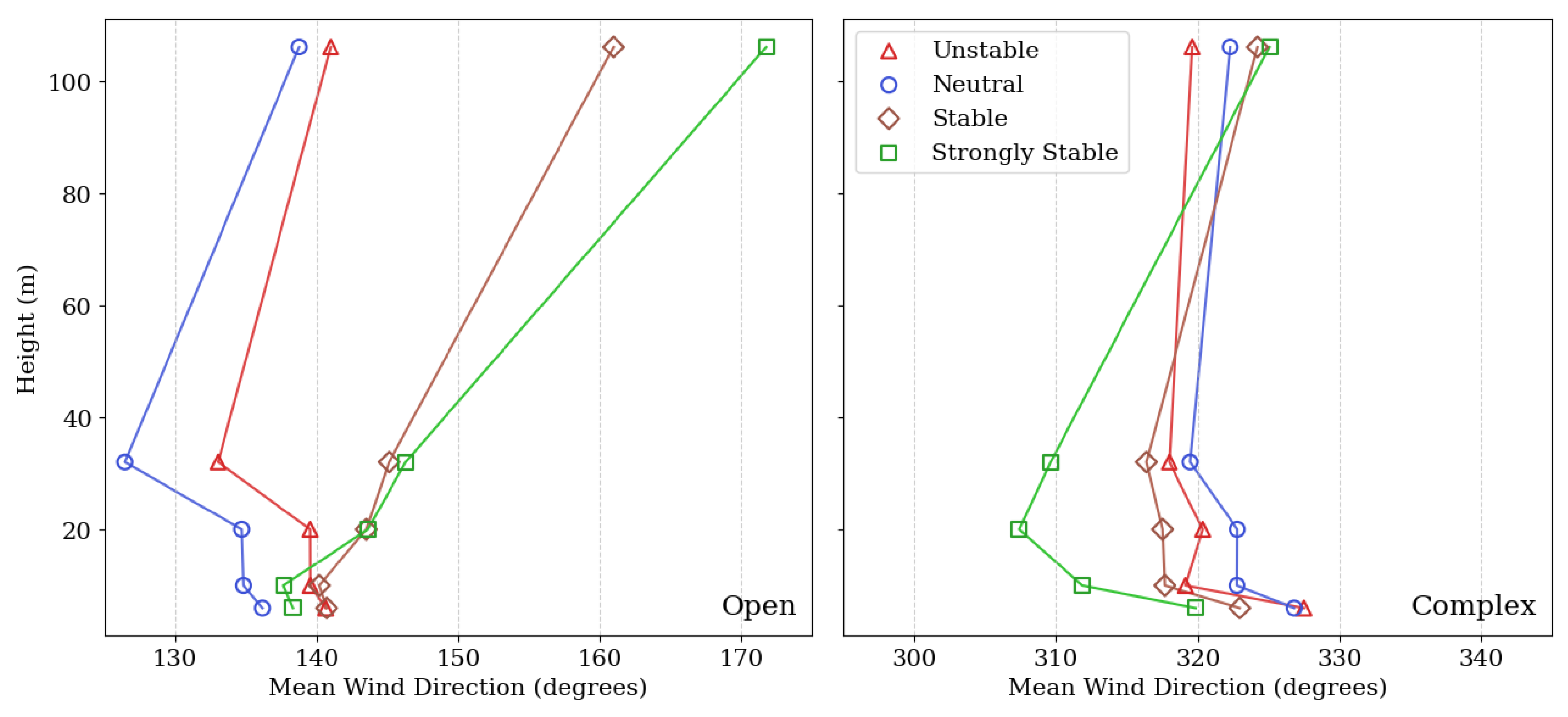
Wind direction is a key factor for optimizing the wind power production. The vertical profiles of mean wind direction, using Z = 10 m as the reference, are shown for different stability classes on the open-field and complex-surface sectors (Figure 12). For the open-field sector (left panel) with unstable and neutral stability, it is interesting that the wind direction is consistent over the height, except at Z = 32 m where wind direction is reduced by 8 degrees. In contrast, for the stable and strongly stable cases, wind direction increases more linearly away from the surface, exhibiting a significant veer. The largest veer is more than 30° in the strongly stable stability class over the open-field terrain. This observation aligns with the results of [46], which documented pronounced wind veer over flat terrain in a stable ABL. Significant veer is rare under neutral stability conditions. For the complex-surface sector (right panel), the wind direction is constant with height for unstable, neutral, and stable stability, except just above the ground. However, under strongly stable condition, wind directions are reduced by around 10° at Z = 10, 20, and 32 m. We suspected that the weaker veer over the complex-surface sector may be due to enhanced turbulence and wakes from local roughness elements (e.g., buildings and trees), which increase vertical mixing and reduce directional variability. Because the directions at greater heights remain generally consistent (relative to the sector size) to those at 10 m, the choice of 60° for open-field or complex-surface wind sectors is confirmed to be reasonable.

3.4. Variation of Horizontal Wind Turbulence Intensity with Height

We have looked at mean wind profiles that are reasonably described using the power-law formulation for two terrains and several thermal stability cases. This section focuses on the turbulence intensity profiles for these terrain and stability conditions and identifies associated fluid flow mechanisms. The horizontal turbulence intensity TI was estimated based on 10 min averaged cup anemometer data, following [49]:
T I = u r m s ( z ) U ( z ) ,
where U ( z ) is the mean wind speed measured at height z, and u r m s is the root-mean-square of the horizontal velocity fluctuations:
u r m s = u ( t ) 2 ¯ .
Due to the low response rate (1 Hz) of a cup anemometer, smaller-scale turbulence would not be captured in the data, which leads to an underestimation of the actual turbulence intensity [50]. Also, the cup data only considers the horizontal components of the wind. In addition, in neutral and unstable cases, the large-scale turbulence captured by cup anemometers is not necessarily of the same scale. Cup anemometers primarily measure the horizontal wind speed fluctuations, neglecting the vertical component of turbulence, which can be significant during unstable conditions.
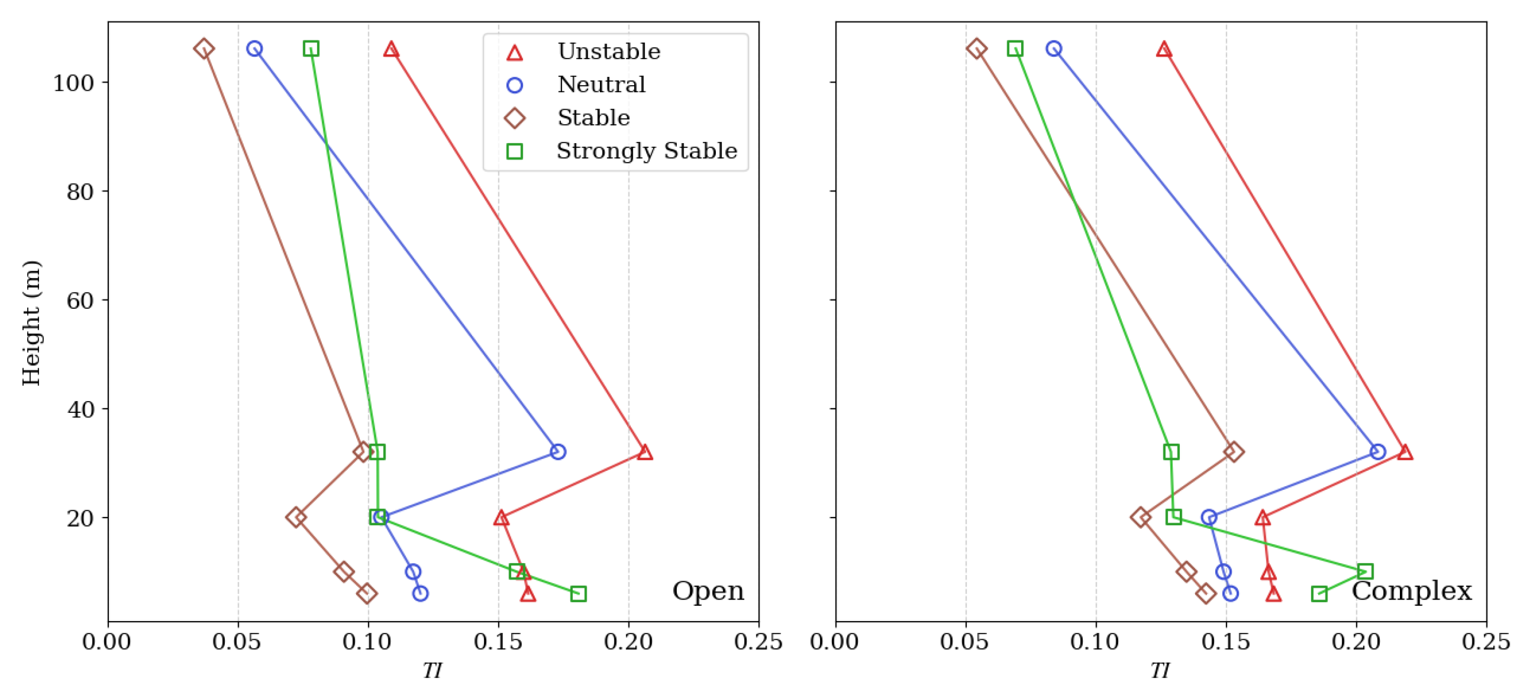
Vertical profiles of horizontal turbulence intensity for the open-field and complex-surface sectors and for each thermal stability condition are shown in Figure 13. Across the different stability cases, the T I magnitude is generally greater over the complex-surface sector than over the open field. The thermal stability effects on the T I magnitude are pronounced. For example, at the lowest altitude (Z = 6 m), T I is about 17% for unstable conditions over open terrain, while it is reduced to 12% and 10% for the neutral and stable conditions, respectively. The remarkable difference in turbulence intensities near the ground reflects the enhanced or suppressed mixing affected by heating or cooling of the surface. For the complex-surface sector, a similar trend is observed. Another observation is that the magnitude of T I over the open and complex-surface sectors is greatest for the strongly stable class, in contrast with other stability classes. This might be explained by the boundary-layer turbulence being developed aloft, away from the surface, and therefore “decoupled” from near-surface structures that are affected more directly by interaction with surface features.
For the unstable, neutral, and stable stability cases, T I displays a maximum at Z = 32 m—well above ground level—deviating from the typical turbulent boundary layer, for which turbulence intensity decreases with height, with the highest value near the surface [24,51]. Typical vertical profiles of T I have been documented in other field studies [36,46,48,52]. The elevated maximum T I at Z = 32 m suggests an influence of local surface features near the met tower. Analysis of the wind sector over the complex surface—including topography and land cover—points to the tree canopy as likely the primary contributor. The 2D elevation transect (see Figure 2) maps topography and surface features up to 500 m along the centerline of the complex-surface sector (northwest, 285°–345°). The oak and maple trees, approximately 15–20 m tall, form a distinct tree line with a terminus about 10 times the canopy height upwind of the met tower.
Prior studies show such abrupt canopy edges can cause flow separation and enhance turbulence up to 15 canopy heights downwind [51,53]. Wind tunnel experiments confirm that canopy-induced wakes produce a sheltered low-speed zone followed by an internal boundary layer (IBL) extending four to six canopy heights downstream [54]. Boom 4 (Z = 32 m), located within this IBL, at roughly twice the canopy height, detects elevated TI likely due to Kelvin–Helmholtz instabilities and IBL development [55]. The shallow hill beneath the trees may further amplify turbulence via slope effects. However, this interpretation remains qualitative, as turbulence is influenced by several factors, including canopy characteristics such as species, porosity, stiffness, and wind reactivity.
Enhanced turbulence intensity is also observed at the height of 32 m above the surface for the open-field sector. This was unexpected, but may be attributed to a row of trees along the adjacent east-to-west roadway, beginning about 30 m south of the met tower and continuing along the road to the east. The row of trees acts as a windbreaks, which could induce significant turbulence due to the high shear between the upper accelerated wind and the lower slowed-down wake region [56,57]. Distributions of annual T I data at each boom and wind sector, as well as variations of T I as a function of wind speed at each boom are provided in the Supplementary Materials. These additional details provide further support for the observed enhancement of turbulence over the complex surface and the pronounced increase at 32 m.

4. Conclusions and Outlook

Accurate characterization of ABL wind profiles—particularly mean wind speed, direction, and turbulence intensity—is critical for the effective deployment and operation of wind energy systems. While numerous studies have examined the wind shear exponent α over relatively flat terrain, its behavior in moderately complex peri-urban landscapes remains less well understood. In particular, the combined effects of terrain complexity and atmospheric thermal stability on α have not been comprehensively explored. To address this gap, the present study investigates how α varies with terrain features and atmospheric stability near the city of Cedar Rapids, Iowa, using 1 year of multiple-level wind measurements from a 106-m meteorological tower.
The power-law model provides a reasonable fit for mean wind profiles at the site. The results show that the wind shear exponent α exhibits more sensitivity to atmospheric stability than to terrain complexity. In general, α increases with increasing bulk Richardson number R i b , reflecting weaker vertical shear under unstable conditions and stronger shear under more stable conditions. Under stable and neutral conditions, the α values were similar across both open-field and complex-surface sectors, but they diverged under unstable and strongly stable conditions. The statistical distribution of α is non-Gaussian across stability regimes, with greater skewness observed for neutral and unstable periods. Median values of α , computed from these distributions, appear to provide a consistent characterization of wind shear and are relatively insensitive to terrain effects. A clear diurnal variation of α was observed, particularly in the summer months, with larger amplitude over open terrain. The variation was less pronounced during the winter months and over the complex-surface sector. Additionally, under strongly stable conditions, profiles of wind direction exhibited significant veer regardless of surface—exceeding 30° over open terrain.
Horizontal turbulence intensity also varied with both the open-field and complex-surface wind sectors and atmospheric stability. Turbulence intensities were generally greater over the complex-surface sector and increased progressively from stable to unstable conditions. Interestingly, the maximum turbulence intensity did not occur near the surface but rather aloft at Z = 32 m, under all stability regimes except the strongly stable case. This turbulence enhancement is attributed to wake turbulence and the associated IBL generated downwind of the tree canopy and terrain features—particularly from the oak and maple trees located several hundred meters upwind in the prevailing northwest sector. Note that the peak turbulence is observed at Boom 4 (32 m). The true location of maximum turbulence may lie above or below 32 m, but it is certainly above 20 m at Boom 3. However, no measurements were taken between Boom 4 and Boom 5 (32–80 m). Future studies could improve the spatial resolution of tower-mounted wind sensors and incorporate remote sensing instruments, such as Doppler wind Lidar, to better resolve turbulence intensity within this region.
The findings underscore the significant influence of local topography and moderate surface heterogeneity on near-surface turbulence. They highlight the need for site-specific evaluation of wind speed and turbulence profiles, especially in peri-urban environments where wake turbulence and the formation of IBLs are common features of the flow. Fixed-location meteorological towers in such settings are inherently limited by spatial variability in boundary layer structure. Therefore, both the measurement height and the tower’s position relative to nearby roughness elements must be carefully considered when analyzing wind data. The wind data at this site could be more valuable when combined with other field datasets for comprehensive studies of winds across varying surface heterogeneity and atmospheric thermal stability. Such integration may help identify general trends and provide insights into theory and unified models for wind energy applications. The goal of this work is to enhance full-scale wind measurement practices, improve interpretation of near-surface wind data, and strengthen predictions of urban and peri-urban wind flow for wind energy applications. The present work contributes to advancing the broader objectives of the energy transition by enabling more efficient, reliable, and sustainable expansion of wind energy. Future research incorporating high-frequency, three-dimensional wind velocity data from sonic anemometers mounted on the same meteorological tower could offer additional insights into small-scale turbulence dynamics.

Supplementary Materials

The following supporting information can be downloaded at: https://www.mdpi.com/article/10.3390/en18195211/s1, Figure S1. Distributions of turbulence intensity at each boom height. Means are shown with vertical lines; Figure S2. Turbulence intensity as a function of wind speed at each boom height (using 0.5 m/s bins).; Data used to plot profiles shown in the figures are included: Table S1. annual_profiles_fig9; Table S2. tod_wse_fig11; Table S3. veer_profiles_fig12; Table S4. ti_profiles_fig13. Reference [58] is cited in the Supplementary Materials.

Author Contributions

Conceptualization, W.Z. and C.D.M.; methodology, W.Z., E.W. and C.D.M.; software, E.W.; formal analysis, W.Z., E.W. and C.D.M.; investigation, W.Z., E.W. and C.D.M.; resources, W.Z. and C.D.M.; data curation, W.Z., E.W. and C.D.M.; writing—original draft preparation, W.Z. and E.W.; writing—review and editing, W.Z., E.W. and C.D.M.; visualization, W.Z., E.W. and C.D.M.; supervision, W.Z. and C.D.M.; project administration, W.Z. and C.D.M.; funding acquisition, W.Z. and C.D.M. All authors have read and agreed to the published version of the manuscript.

Funding

This research was funded by the National Science Foundation (NSF) CAREER [Award #2533282]; NSF Great Lakes Wind Energy Challenges REU Site [Award #215000]; NSF Iowa EPSCoR [Award #1101284]; and the Center For Global & Regional Environmental Research (CGRER), University of Iowa.

Data Availability Statement

Data is contained within the article or Supplementary Materials.

Acknowledgments

The authors thank Kirkwood Community College for providing access to the transmission tower and wind turbine as well as providing assistance with instrument deployment. We also acknowledge the Iowa Environmental Mesonet (https://mesonet.agron.iastate.edu/, accessed on 27 January 2025) for making the CID airport data available. W. Zhang acknowledges the support of the National Science Foundation (NSF) CAREER grant (Award #2533282). E. Walker acknowledges the support of the NSF Great Lakes Wind Energy Challenges REU Site (Award #215000). C. D. Markfort acknowledges funding from NSF Iowa EPSCoR (Award #1101284) and the Center For Global & Regional Environmental Research (CGRER), University of Iowa.

Conflicts of Interest

The authors declare no conflicts of interest.

References

  1. Cole, W.J.; Greer, D.; Denholm, P.; Frazier, A.W.; Machen, S.; Mai, T.; Vincent, N.; Baldwin, S.F. Quantifying the challenge of reaching a 100% renewable energy power system for the United States. Joule 2021, 5, 1732–1748. [Google Scholar] [CrossRef]
  2. Denholm, P.; Arent, D.J.; Baldwin, S.F.; Bilello, D.E.; Brinkman, G.L.; Cochran, J.M.; Cole, W.J.; Frew, B.; Gevorgian, V.; Heeter, J.; et al. The challenges of achieving a 100% renewable electricity system in the United States. Joule 2021, 5, 1331–1352. [Google Scholar] [CrossRef]
  3. Larson, E. Net-Zero America: Potential Pathways, Infrastructure, and Impacts; Princeton University: Princeton, NJ, USA, 2020. [Google Scholar]
  4. Banta, R.; Pichugina, Y.; Kelley, N.; Michael Hardesty, R.; Alan Brewer, W. Wind Energy Meteorology: Insight into Wind Properties in the Turbine-Rotor Layer of the Atmosphere from High-Resolution Doppler Lidar. Bull. Am. Meteorol. Soc. 2013, 94, 883–902. [Google Scholar] [CrossRef]
  5. Dechamps, P. The IEA World Energy Outlook 2022—A brief analysis and implications. Eur. Energy Clim. J. 2023, 11, 100–103. [Google Scholar] [CrossRef]
  6. Veers, P.; Dykes, K.; Lantz, E.; Barth, S.; Bottasso, C.L.; Carlson, O.; Clifton, A.; Green, J.; Green, P.; Holttinen, H.; et al. Grand challenges in the science of wind energy. Science 2019, 366, eaau2027. [Google Scholar] [CrossRef]
  7. Porté-Agel, F.; Bastankhah, M.; Shamsoddin, S. Wind-Turbine and Wind-farm Flows: A review. Bound.-Layer Meteorol. 2020, 174, 1–59. [Google Scholar] [CrossRef]
  8. Clifton, A.; Barber, S.; Stökl, A.; Frank, H.; Karlsson, T. Research challenges and needs for the deployment of wind energy in hilly and mountainous regions. Wind. Energy Sci. 2022, 7, 2231–2254. [Google Scholar] [CrossRef]
  9. Zhang, W.; Markfort, C.D.; Porté-Agel, F. Wind-tunnel experiments of turbulent wind fields over a two-dimensional (2d) steep hill: Effects of the stable boundary layer. Bound.-Layer Meteorol. 2023, 188, 441–461. [Google Scholar] [CrossRef]
  10. Revaz, T.; Porté-Agel, F. Effect of hills on wind turbine flow and power efficiency: A large-eddy simulation study. Phys. Fluids 2024, 36, 95180. [Google Scholar] [CrossRef]
  11. Markfort, C.D.; Zhang, W.; Porté-Agel, F. Analytical Model for Mean Flow and Fluxes of Momentum and Energy in Very Large Wind Farms. Bound.-Layer Meteorol. 2018, 166, 31–49. [Google Scholar] [CrossRef]
  12. Riva, A.D.; Hethey, J.; Lüers, S.; Wallasch, A.K.; Rehfeldt, K.; Duffy, A.; Weir, D.E.; Stenkvist, M.; Uihlein, A.; Stehly, T.J.; et al. IEA Wind TCP Task 26—Wind Technology, Cost, and Performance Trends in Denmark, Germany, Ireland, Norway, Sweden, the European Union, and the United States: 2008–2016; Technical Report; National Renewable Energy Laboratory (NREL): Golden, CO, USA, 2018. [Google Scholar]
  13. Bilgili, M.; Alphan, H. Global growth in offshore wind turbine technology. Clean Technol. Environ. Policy 2022, 24, 2215–2227. [Google Scholar] [CrossRef]
  14. Saint-Drenan, Y.M.; Besseau, R.; Jansen, M.; Staffell, I.; Troccoli, A.; Dubus, L.; Schmidt, J.; Gruber, K.; Simões, S.G.; Heier, S. A parametric model for wind turbine power curves incorporating environmental conditions. Renew. Energy 2020, 157, 754–768. [Google Scholar] [CrossRef]
  15. Vahidzadeh, M.; Markfort, C.D. Modified power curves for prediction of power output of wind farms. Energies 2019, 12, 1805. [Google Scholar] [CrossRef]
  16. Wagner, R.; Courtney, M.; Gottschall, J.; Lindelöw-Marsden, P. Accounting for the speed shear in wind turbine power performance measurement. Wind Energy 2011, 14, 993–1004. [Google Scholar] [CrossRef]
  17. Choukulkar, A.; Pichugina, Y.; Clack, C.T.; Calhoun, R.; Banta, R.; Brewer, A.; Hardesty, M. A new formulation for rotor equivalent wind speed for wind resource assessment and wind power forecasting. Wind Energy 2016, 19, 1439–1452. [Google Scholar] [CrossRef]
  18. Howland, M.F.; Lele, S.K.; Dabiri, J.O. Wind farm power optimization through wake steering. Proc. Natl. Acad. Sci. USA 2019, 116, 14495–14500. [Google Scholar] [CrossRef]
  19. Kosović, B.; Basu, S.; Berg, J.; Berg, L.K.; Haupt, S.E.; Larsén, X.G.; Peinke, J.; Stevens, R.J.; Veers, P.; Watson, S. Impact of atmospheric turbulence on performance and loads of wind turbines: Knowledge gaps and research challenges. Wind. Energy Sci. Discuss. 2025, 2025, 1–67. [Google Scholar]
  20. Vahidzadeh, M.; Markfort, C.D. An induction curve model for prediction of power output of wind turbines in complex conditions. Energies 2020, 13, 891. [Google Scholar] [CrossRef]
  21. Touma, J.S. Dependence of the wind profile power law on stability for various locations. J. Air Pollut. Control. Assoc. 1977, 27, 863–866. [Google Scholar] [CrossRef]
  22. Fernando, H.J.S. Fluid Dynamics of Urban Atmospheres in Complex Terrain. Annu. Rev. Fluid Mech. 2010, 42, 365–389. [Google Scholar] [CrossRef]
  23. Kaimal, J.K.; Finnigan, J. Atmospheric Boundary Layer Flows: Their Structure and Measurement; Oxford University Press: Oxford, UK, 1994. [Google Scholar]
  24. Stull, R.B. An Introduction to Boundary Layer Meteorology; Kluwer Academic Publishers: Dordrecht, The Netherlands, 1988. [Google Scholar]
  25. Grimmond, C.; Oke, T. Aerodynamic Properties of Urban Areas Derived from Analysis of Surface Form. J. Appl. Meteorol. Climatol. 1999, 38, 1262–1291. [Google Scholar] [CrossRef]
  26. Giometto, M.G.; Christen, A.; Egli, P.E.; Schmid, M.F.; Tooke, R.T.; Coops, N.C.; Parlange, M.B. Effects of trees on mean wind, turbulence and momentum exchange within and above a real urban environment. Adv. Water Resour. 2017, 106, 154–168. [Google Scholar] [CrossRef]
  27. Lopez-Villalobos, C.A.; Martinez-Alvarado, O.; Rodriguez-Hernandez, O.; Romero-Centeno, R. Analysis of the influence of the wind speed profile on wind power production. Energy Rep. 2022, 8, 8079–8092. [Google Scholar] [CrossRef]
  28. IEC 61400-1:2019; Wind Energy Generation Systems—Part 1: Design Requirements. International Electrotechnical Commission: Geneva, Switzerland, 2019.
  29. IEC 61400-2:2013; Wind Energy Generation Systems—Part 2: Design Requirements for Small Wind Turbines. International Electrotechnical Commission: Geneva, Switzerland, 2013.
  30. Davenport, A. The Relationship of Wind Structure to Wind Loading. In Proceedings of the National Physical Laboratory, Symposium No. 16, Wind Effects on Buildings and Structures, London, UK, 26–28 June 1963; pp. 54–102. [Google Scholar]
  31. Drew, D.; Barlow, J.; Cockerill, T. Estimating the potential yield of small wind turbines in urban areas: A case study for Greater London, UK. J. Wind. Eng. Ind. Aerodyn. 2013, 115, 104–111. [Google Scholar] [CrossRef]
  32. Lange, J.; Mann, J.; Berg, J.; Parvu, D.; Kilpatrick, R.; Costache, A.; Chowdhury, J.; Siddiqui, K.; Hangan, H. For wind turbines in complex terrain, the devil is in the detail. Environ. Res. Lett. 2017, 12, 094020. [Google Scholar] [CrossRef]
  33. Sathe, A.; Bierbooms, W. Influence of different wind profiles due to varying atmospheric stability on the fatigue life of wind turbines. J. Phys. Conf. Ser. 2007, 75, 12056. [Google Scholar] [CrossRef]
  34. Honrubia, A.; Vingueras-Rodriguez, A.; Lazaro, E.G.; Rodríguez, D.; Mejias, M.; Lainez, I. The influence of wind shear in wind turbine power estimation. Measurements 2010, 2, 9. [Google Scholar]
  35. Newman, J.F.; Klein, P.M. The impacts of atmospheric stability on the accuracy of wind speed extrapolation methods. Resources 2014, 3, 81–105. [Google Scholar] [CrossRef]
  36. Gualtieri, G. Surface turbulence intensity as a predictor of extrapolated wind resource to the turbine hub height. Renew. Energy 2015, 78, 68–81. [Google Scholar] [CrossRef]
  37. Gualtieri, G. Atmospheric stability varying wind shear coefficients to improve wind resource extrapolation: A temporal analysis. Renew. Energy 2016, 87, 376–390. [Google Scholar] [CrossRef]
  38. Ahlman, R.M.; Zhang, W.; Markfort, C.D. Effects of terrain and atmospheric thermal stability on wind velocity profiles. In ASTFE Digital Library; Begel House Inc.: Danbury, CT, USA, 2021. [Google Scholar]
  39. IEC 61400-12-1:2022; Wind Energy Generation Systems—Part 12-1: Power Performance Measurements of Electricity Producing Wind Turbines. International Electrotechnical Commission: Geneva, Switzerland, 2022.
  40. Albornoz, C.P.; Soberanis, M.E.; Rivera, V.R.; Rivero, M. Review of atmospheric stability estimations for wind power applications. Renew. Sustain. Energy Rev. 2022, 163, 112505. [Google Scholar] [CrossRef]
  41. Mauritsen, T.; Svensson, G. Observations of stably stratified shear-driven atmospheric turbulence at low and high Richardson numbers. J. Atmos. Sci. 2007, 64, 645–655. [Google Scholar] [CrossRef]
  42. Murray, F. On the Computation of Saturation Vapor Pressure. J. Appl. Meteorol. 1967, 6, 203–204. [Google Scholar] [CrossRef]
  43. Gualtieri, G. A comprehensive review on wind resource extrapolation models applied in wind energy. Renew. Sustain. Energy Rev. 2019, 102, 215–233. [Google Scholar] [CrossRef]
  44. Emeis, S. Wind Energy Meteorology: Atmospheric Physics for Wind Power Generation; Springer: Berlin/Heidelberg, Germany, 2018. [Google Scholar]
  45. Irwin, J. A theortical variation of the wind profile power-law exponent as a function of surface roughness and stability. Atmos. Environ. 1978, 13, 191–194. [Google Scholar] [CrossRef]
  46. Kelley, C.L.; Ennis, B.L. SWiFT Site Atmospheric Characterization; Technical Report; Sandia National Lab. (SNL-NM): Albuquerque, NM, USA, 2016. [Google Scholar]
  47. Smith, K.; Randall, G.; Malcom, D.; Kelley, N.; Smith, B. Evaluation of Wind Shear Patterns at Midwest Wind Energy Facilities (NREL/CP-500-32492); American Wind Energy Association (AWEA): Portland, OR, USA, 2002. [Google Scholar]
  48. Rehman, S.; Al-Abbadi, N.M. Wind shear coefficient, turbulence intensity and wind power potential assessment for Dhulom, Saudi Arabia. Renew. Energy 2008, 33, 2653–2660. [Google Scholar] [CrossRef]
  49. Clifton, A.; Schreck, S.; Scott, G.; Kelley, N.; Lundquist, J.K. Turbine inflow characterization at the national wind technology center. J. Sol. Energy Eng. 2013, 135, 031017. [Google Scholar] [CrossRef]
  50. Brock, F.V.; Richardson, S.J. Meteorological Measurement Systems; Oxford University Press: New York, NY, USA, 2001. [Google Scholar]
  51. Emeis, S. Current issues in wind energy meteorology. Meteorol. Appl. 2014, 21, 803–819. [Google Scholar] [CrossRef]
  52. Gao, L.; Yang, S.; Abraham, A.; Hong, J. Effects of inflow turbulence on structural response of wind turbine blades. J. Wind. Eng. Ind. Aerodyn. 2020, 199, 104137. [Google Scholar] [CrossRef]
  53. Träumner, K.; Wieser, A.; Ruck, B.; Frank, C.; Röhner, L.; Kottmeier, C. The suitability of Doppler lidar for characterizing the wind field above forest edges. Forestry 2012, 85, 399–411. [Google Scholar] [CrossRef]
  54. Markfort, C.D.; Porté-Agel, F.; Stefan, H.G. Canopy-wake dynamics and wind sheltering effects on Earth surface fluxes. Environ. Fluid Mech. 2014, 14, 663–697. [Google Scholar] [CrossRef]
  55. Kanani, F.; Träumner, K.; Ruck, B.; Raasch, S. What determines the differences found in forest edge flow between physical models and atmospheric measurements? An LES study. Meteorol. Z. 2014, 23, 33–49. [Google Scholar] [CrossRef]
  56. Wang, H.; Takle, E.S.; Shen, J. Shelterbelts and windbreaks: Mathematical modeling and computer simulations of turbulent flows. Annu. Rev. Fluid Mech. 2001, 33, 549–586. [Google Scholar] [CrossRef]
  57. McClure, S.; Kim, J.J.; Lee, S.J.; Zhang, W. Shelter effects of porous multi-scale fractal fences. J. Wind. Eng. Ind. Aerodyn. 2017, 163, 6–14. [Google Scholar] [CrossRef]
  58. Peña, A.; Mirocha, J.D. One-year-long turbulence measurements and modeling using large-eddy simulation domains in the Weather Research and Forecasting model. Appl. Energy 2024, 363, 123069. [Google Scholar] [CrossRef]
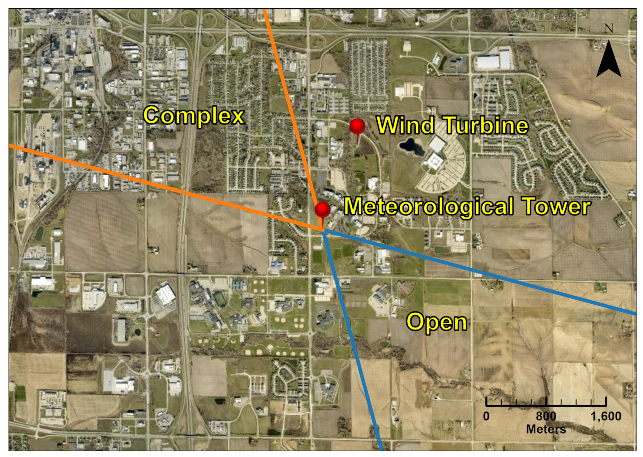
Figure 1. Aerial image showing the location of the meteorological tower and the wind turbine at the Kirkwood Community College in Cedar Rapids, Iowa, with 60°-wide wind sectors overlaid.
Energies 18 05211 g001
Figure 2. Schematic of the flow regimes induced by the tree canopies over the shallow hill along the center line of the northwest wind sector (i.e., complex surface) upwind of the met tower.
Energies 18 05211 g002
Figure 3. The meteorological tower at the Kirkwood Community College in Cedar Rapids, Iowa (left); schematic diagram of arrangement of various sensors on the met tower (right).
Energies 18 05211 g003
Figure 4. Wind speed and direction data availability at each boom (shown in blue) across a 1-year duration. Time periods without data are shown in red.
Energies 18 05211 g004
Figure 5. Wind roses generated from the data collected between Sept 2017 and Sept 2018 at 10 m above ground level at the KCC met tower (left) and the nearby CID airport (right).
Energies 18 05211 g005
Figure 6. Comparison of temperature recorded from the 106 m meteorological tower and Cedar Rapids Airport weather station, with data clustered about the 1:1 line.
Energies 18 05211 g006
Figure 7. Quantity of wind data sorted by thermal stability classification based on R i b .
Energies 18 05211 g007
Figure 8. Probability density distribution of annual wind speed over open-field and complex-surface sectors at various heights. Weibull distributions are overlaid, with shape parameter k and scale parameter λ indicated in the upper-right corner of each subplot.
Energies 18 05211 g008
Figure 9. Vertical profiles of the mean wind speed with best-fit power-law functions: Open-field sector (southeast 105°–165°, (left)) and complex-surface sector (northwest 285°–345°, (right)).
Energies 18 05211 g009
Figure 10. Probability density of the wind shear exponent α according to thermal stability and wind sectors. Medians are marked with dashed vertical lines.
Energies 18 05211 g010
Figure 11. Diurnal variation of wind shear exponent α according to season and direction classification. Error bars show the standard deviation of α across that same sample, and green dashed lines indicate local sunrise/sunset times at the middle (equinox or solstice) of each season for reference.
Energies 18 05211 g011
Figure 12. Vertical profiles of mean wind direction over open (left) and complex (right) terrain.
Energies 18 05211 g012
Figure 13. Vertical profiles of horizontal turbulence intensity T I , over open (left) and complex (right) terrain. Distributions of T I at each boom are included in the Supplementary Materials.
Energies 18 05211 g013
Table 1. List of instruments on the 106 m meteorological tower.
SensorMake/ModelQuantityHeights (m)Sampling Rate (Hz)
Barometric PressureSetra 27826, 1061
Temperature SensorNRG 110S26, 201
Wind VaneNRG 200P76, 10, 20, 32, 80, 1061
Cup AnemometerA100LK76, 10, 20, 32, 80, 1061
Temp./RH SensorVaisala-HMP 155410, 32, 80, 1061
Sonic AnemometerCampbell Scientific-CSAT3B410, 32, 80, 10620
Table 2. Wind shear exponent α for different thermal stability conditions and terrain cases. In Kelley and Ennis [46], neutral stability is defined for | R i b | < 0.02.
CaseUnstableNeutralStableStrongly Stable
Open Complex Open Complex Open Complex Open Complex
Median value of α (Figure 10)0.110.170.240.250.390.400.450.39
Mean value of α (Figure 10)0.120.170.250.260.400.410.450.41
α (mean profiles in Figure 9)0.130.170.240.250.380.390.440.39
α (Oklahoma Mesonet, [35])0.090.130.280.39
α (tall tower, [35])0.080.160.260.28
α (TTU 200 m tower, [46])0.050.1250.3
Median R i b −1.01−0.380.00−0.020.170.160.480.54
Disclaimer/Publisher’s Note: The statements, opinions and data contained in all publications are solely those of the individual author(s) and contributor(s) and not of MDPI and/or the editor(s). MDPI and/or the editor(s) disclaim responsibility for any injury to people or property resulting from any ideas, methods, instructions or products referred to in the content.