Large-Scale Transmission Expansion Planning with Network Synthesis Methods for Renewable-Heavy Synthetic Grids

Abstract

With increasing electrification and the connection of more renewable resources at the transmission level, bulk interconnected electric grids need to plan network expansion with new transmission facilities. The transmission expansion planning (TEP) problem is particularly challenging because of the combinatorial, integer optimization nature of the problem and the complexity of engineering analysis for any one possible solution. Network synthesis methods, that is, heuristic-based techniques for building synthetic electric grid models based on complex network properties, have been developed in recent years and have the capability of balancing multiple aspects of power system design while efficiently considering large numbers of candidate lines to add. This paper presents a methodology toward scalability in addressing the large-scale TEP problem by applying network synthesis methods. The algorithm works using a novel heuristic method, inspired by simulated annealing, which alternates probabilistic removal and targeted addition, balancing the fixed cost of transmission investment with objectives of resilience via power flow contingency robustness. The methodology is demonstrated in a test case that expands a 2000-bus interconnected synthetic test case on the footprint of Texas with new transmission to support 2025-level load and generation.

1. Introduction

Increased electrification and the interconnection of new renewable generation will require significant expansion of the electric transmission grid over the next 5–20 years [1]. Many regions worldwide are performing studies to explore potential expansion options, for example, in the US state of Texas, a recent study showed a variety of expansion options to the 345 kV network and a possible new 765 kV network [2], as the state expects a doubling of load over the next 5–10 years and a commensurate growth in generation. As another example, Australia has announced a major investment in the transmission network as part of the “Rewire the Nation” initiative [3].

There are several important challenges fundamental to transmission expansion planning (TEP) for practical, large-scale electric grid networks. The problem is inherently discrete—you cannot build a fraction of a transmission line—and the number of possibilities scales combinatorially. There are nearly uncountable possible transmission grids that could be built. On top of this challenge, investigating the viability of even one possible solution requires a thorough engineering analysis, considering the cost–benefit tradeoffs and ensuring grid robustness is adequate across a range of requirements and contingencies. For this reason, integer programming-based methods, as currently developed, have been applied very little in industry. Instead, a relatively small number of possibilities are selected by engineering judgment, and then a detailed analysis is made of each one [1,2].

Electric grids are complex networks, that is, large-scale graphs with emergent properties that can be associated with their function and performance. The complex network framework has applicability not only in the area of grid analysis, but also for grid design. Network synthesis methods, originally developed for use in building synthetic grids from scratch as test cases [4,5], have leveraged this paradigm to produce scalable branch selection algorithms incorporating numerous and varied constraints, including geographic features, geometric distances, power flow, contingency conditions, and graph properties. Such considerations are quite similar to the goals of the TEP problem. Therefore, the objective of this paper is to outline and demonstrate a new methodology based on network synthesis methods toward solving TEP problems for large-scale, renewable-heavy networks that need long-term expansion planning to meet new load and generation growth.

1.1. Literature Review on the TEP Problem and Research Gaps

TEP seeks to augment an already existing electric network with the optimal lowest-cost set of new transmission lines, transformers, and substations, which will sufficiently serve new generation and load with adequate reliability. This problem has been studied in various forms for several decades. The purpose of this subsection is to review the key features of state-of-the-art methods for TEP solving and explain how the proposed novel approach fits in. The reader is referred to [6,7] for a more comprehensive review.

The most natural formulation of the TEP is as a mixed integer linear programming (MILP) problem. Although the problem is not inherently linear, appropriate linearizations can generally be made, since the focus of the problem is on real power flows. The advantage of this approach is that state-of-the art, general-purpose MILP solvers can be employed. One example is [8], in which the authors included transmission contingencies into a MILP formulation to make decisions about 17 candidate lines to possibly be added to an IEEE 118-bus case. Another example is [9], which considered energy storage decisions and addressed losses with chord- and secant-based linear approximations. Other works have combined generation and transmission expansion [10,11] and specifically attempted to address nonlinearities in a MILP context with piecewise linear modeling [12].

To handle nonlinearities, check feasibility, and address scalability challenges, many TEP solution approaches involve a primary–secondary subproblem structure using, for instance, a generalized Benders decomposition [13,14]. An alternative strategy is to use an outer-loop nonlinear analysis that reformulates and corrects the inner MILP [15,16].

More complex structures similar to this one are necessary when the TEP formulation is designed to handle various modeling complexities. For example, in [17,18], multiple timepoints were considered in sequence, greatly expanding the scale of the problem, and hence outer-loop and more complex structures were required. Similarly, in [19,20,21] and many other similar works, the inherent stochasticity and uncertainty involved in wind, solar, and load also have the effect of adding additional variables and constraints to the multi-horizon TEP.

Of particular interest in this work is the impact of contingency constraints—the network structure is heavily impacted by these. Common methods for dealing with these include multi-level problem strategies [22] and adding reliability metrics as constraints [23]. In [24], the authors modeled potential operator actions in the third lowest-level problem and used robust optimization to account for the worst-case N–k conditions. An alternative method was given in [25], in which the contingency conditions were moved from constraints to the objective itself in the form of the risk of disconnecting the system—that is, the objective was to minimize the blackout probability. Interesting variations on this problem include the consideration of variable branch reactances [26] and dynamic transmission switching [27].

As mentioned, direct integer programming methods for finding the optimal solutions to the associated MILPs generally suffer from scalability challenges for the TEP problem. Hence, there are also many works utilizing metaheuristics [28], such as simulated annealing [29], particle swarm optimization [30,31,32], evolutionary algorithms [33,34], and others [35,36]. Some efforts have used nonlinear programming techniques directly, such as [37].

A continuing challenge in all of the literature reviewed is scalability. Generally, these frameworks have a pool of about 50 candidate lines, or, in some cases, much fewer.

Table 1. TEP problem scalability in the recent literature.

Reference	Buses in the Largest Case	Candidate Lines Considered in the Largest Case	Year
[22]	24	105	2023
[27]	24	123	2020
[32]	17	19	2021
[37]	93	24	2022
[39]	118	186	2020
[40]	271	376	2024

shows problem scalability in some of the more recent TEP papers from the literature. The complex network theory, which explores emergent graph properties of large-scale real-world networks, was applied in [38,39,40] to the TEP. These studies showed that complex network metrics can help with understanding a broader range of candidate lines, reducing the search space and helping to understand the impacts of particular candidate branches on objective components.

Geographically based network synthesis methods for power systems have emerged in recent years, applying both a range of complex metrics and geographic or geometric properties along with engineering analysis to make realistic test cases for research that match characteristics of realism better than traditional test cases, such as the IEEE test cases, but do not contain critical energy infrastructure information (CEII) as do real electric grid models [3,4,41,42,43]. While such network synthesis methods have, to this point, been applied primarily for creating realistic test cases, their ability to handle scalability and address various aspects of the network generation challenge made them well-suited for the present work, which sought to apply them to very large-scale transmission expansion problems.

The rest of the paper is organized as follows. In Section 2, the network expansion methodology is presented. First, the problem formulation is given, starting with the substation planning stage, load, and generation; then the transmission planning formulation follows. Second, the solution algorithm is derived based on network synthesis methods. Third, a mention of the impact on system dynamics is presented. In Section 3, there is a case study on the Texas2k synthetic grid, a realistic, large-scale test case on the footprint of the US state of Texas. This synthetic case serves to demonstrate the algorithm on a geographically embedded system with the size and detail of actual grid models and allows the final case as well as the problem data to be made available online. Finally, Section 4 concludes the paper.

1.2. Background: Network Synthesis in the Synthetic Grid Building Problem

The synthetic grid building problem [4,5,41,42,43] has many features in common with the TEP problem, but there are differences as well. Synthetic grids start from scratch; the task is to build an entire, fictitious network (on some realistic geography), making decisions about where all transmission facilities go. The TEP problem is, of course, making decisions about new transmission facilities, but the design is highly constrained by the existing network. Synthetic grids also have “realism” as their objective, a difficult-to-define target that essentially means statistical similarity to the existing actual grids (see [43]). Hence, in principle, synthetic grid building does not seek to produce the best and most efficient grid that could possibly be built—indeed, such a grid would be unrealistic, as many factors in the historical development of the actual grid make it sub-optimal when compared to a theoretical ground-up design. However, in the TEP problem, we do want the best possible design, subject to various constraints, including the existing infrastructure.

It is important to note at this point that the scope and focus of the TEP problem under consideration for this paper is early-stage, conceptual planning. These are the types of problems for which high scalability is of great value, and for which few adequate systematic methodologies have been produced. Planning of a large grid’s transmission network for the future begins by looking 10–20 years into the future and attempting to understand the issues that will be relevant and the types and locations of new transmission facilities that will be required. Then, in 1–3 years, the exact new transmission project selection must be made, requiring highly detailed analysis, which is out of scope of the present methodology.

2. Network Expansion Methodology

This section presents both the formulation and the solution algorithm for the network synthesis-based TEP solution methodology. In applying synthetic grid building to the TEP problem, it should be noted that synthetic grid building, at least as formulated in [4] and other studies, creates synthetic networks with a process that mimics the real-world process of transmission planning. The process begins with generation and substation planning—with synthetic grids, this involves using public data to place generators and loads, then clustering them into substations. Then, the second stage—of emphasis here—is transmission planning, focusing on the real power flow. Finally, a reactive power planning stage determines a good location for shunts and other reactive power resources so that there is good power flow convergence and voltage control, followed by additional features such as transient dynamic models.

2.1. Problem Formulation: Transmission Decisions and Objective

This subsection gives the TEP problem formulation as addressed by the methodology proposed in this paper. Following an assessment of generation, load, substation placement, and targeted voltage levels (depending on the specific scenario being studied), the TEP seeks to find the best set of connecting transmission lines that maximizes the ability to serve the electrical load in base and contingency conditions at the lowest possible investment cost. In particular, we defined nodes:

$$i\in \mathcal{N},$$

(1)

which are connected by edges, consisting both of the pre-existing and added transmission lines:

$$\mathcal{l}\in \mathcal{E}={\mathcal{E}}_0+{\mathcal{E}}_{+}$$

(2)

Then, we formed a graph $\mathcal{G}=<\mathcal{N},\mathcal{E}>$. The selected edges ${\mathcal{E}}_{+}$ are a subset of the candidate bank of transmission lines, predefined in some way. The selection of lines is indicated by a binary vector $u$ with length equal to $\left|{\mathcal{E}}_c\right|$, where $u_{\mathcal{l}}\in \left[\mathrm{0,1}\right]$:

$${\mathcal{E}}_{+}=\left\{\mathcal{l}\in {\mathcal{E}}_c|u_{\mathcal{l}}=1\right\}$$

(3)

Hence, by the line selection embedded in the decision variables $u$, the topology of $\mathcal{G}$ is changed.

For each candidate line $\mathcal{l}\in {\mathcal{E}}_c$, we can define several relevant parameters. First, $e_{\mathcal{l}}$ is a vector of length equal to $n=\left|\mathcal{N}\right|-1$, with a = 1 at the line’s associated “from node” and a = −1 at the line’s associated “to node,” the single slack node excepted. Scalar values $s_{lim,\mathcal{l}}$ and $b_{\mathcal{l}}$ are the maximum flow capability and the susceptance value, respectively. Additionally, the line has a fixed cost to construct, $f_{\mathcal{l}}$.

Topological analysis of the graph $\mathcal{G}$ can be performed with a simple depth-first search, to first determine if $\mathcal{G}$ is connected, second, to identify bridges ${\mathcal{E}}_h\subset \mathcal{E}$, and third, to identify radial buses ${\mathcal{N}}_r\subset \mathcal{N}.$ Bridges are lines in the network which, if removed, would divide the network into two components, so that the graph would no longer be connected. Radial buses are those nodes that do not have at least two edge-independent paths to the slack node. That is, with the removal of at least one bridge edge, the node in ${\mathcal{N}}_r$ would lack a path to the slack (root) node. We also would have non-bridges ${\mathcal{E}}_{h^{\prime }}+{\mathcal{E}}_h=\mathcal{E}$ and non-radial nodes ${\mathcal{N}}_{r^{\prime }}+{\mathcal{N}}_r=\mathcal{N}$.

Power flow analysis begins with the assumption of a power operation dispatch point, found from prior economic analysis of the system. This is defined by a vector $p$ of length $n$. The linearized power flow can be performed by solving the equation $B\theta =p$, to get $\theta$, also of length $n$, specifying bus angles in the given dispatch. Susceptance matrix $B$ depends on the graph and the scenario. For the base case, we define the following:

$$B_0=\sum _{\mathcal{l}\in {\mathcal{E}}_0}{e}_{\mathcal{l}}{e}_{\mathcal{l}}^T{b}_{\mathcal{l}}+\sum _{\mathcal{l}\in {\mathcal{E}}_c}{u}_{\mathcal{l}}{e}_{\mathcal{l}}{e}_{\mathcal{l}}^T{b}_{\mathcal{l}}=\sum _{\mathcal{l}\in \mathcal{E}}{e}_{\mathcal{l}}{e}_{\mathcal{l}}^T{b}_{\mathcal{l}}$$

(4)

We also define contingency conditions $k_{\mathcal{l}}$ as the outage of branch $\mathcal{l}$, defining contingency sets as follows:

$$k\in {\mathcal{K}}_{\mathcal{X}},$$

(5)

where $\mathcal{X}$ could be one of the specifications of an edge set, $0$, $+$, $c$, $h$, $h\prime$, etc. To get the susceptance matrix for contingency $k_{\mathcal{l}}$, we use the following Equation:

$$B_{\left(k_{\mathcal{l}}\right)}=B_0-e_{\mathcal{l}}{e}_{\mathcal{l}}^T{b}_{\mathcal{l}}$$

(6)

The angles in that contingency are defined as follows:

$${\theta }_k=B_k^{-1}p$$

(7)

The flows in a branch $\mathcal{l}$ in a contingency $k$ can be found as follows:

$$s_{k,\mathcal{l}}=\left|{\theta }_k^T{e}_{\mathcal{l}}{b}_{\mathcal{l}}\right|$$

(8)

The overload flows are defined as follows:

$$s_{ovr,k,\mathcal{l}}=\mathrm{m}\mathrm{a}\mathrm{x}(0,s_{k,\mathcal{l}}-s_{lim,\mathcal{l}})$$

(9)

Now the appropriate formulation is in place to begin to define the optimization problem for TEP that is addressed by this paper. The objective is to minimize the total cost, which has three parts. First, the total fixed cost $z_f$ is defined as follows:

$$z_f=u^{T}f$$

(10)

Recall that $f$ is a vector that defines the fixed cost for each candidate line, $f_{\mathcal{l}}$. This inner product with the decision variable sums the total fixed cost of all lines.

Second, the total cost of the radial load $z_r$, which depends on how the topology defines the radial set ${\mathcal{N}}_r$ (which varies with $u$) and the associated load at each bus. A scalar parameter $c_{rad}$ is used to define how important to the solution it is to remove the radial load, since the importance of this factor may vary relative to the system being designed and dimensional considerations:

$$z_r=c_{rad}\sum _{i\in {\mathcal{N}}_r}\mathrm{m}\mathrm{a}\mathrm{x}(0,p_i)$$

(11)

Third, the contingency overload costs $z_c$. Contingencies with bridge lines do not allow for a solved system, so only non-bridge contingencies are allowed. To better normalize for variation in the number of contingencies that may be available, the infinity norm is effectively used, measuring for each branch its maximum overload in any contingency. This factor is most influenced by $s_{ovr,k,\mathcal{l}}$, the overload of line $\mathcal{l}$ in contingency $k$. A scalar parameter $c_{over}$ is used to define how important to the solution it is to remove contingency overloads:

$$z_c=c_{ovr} \sum _{\mathcal{l}\in \mathcal{E}}\underset{k\in {\mathcal{K}}_{h^{\prime }}}{\max }\left(s_{ovr,k,\mathcal{l}}\right)$$

(12)

The only hard constraint on the problem is that $\mathcal{G}$ must be a connected graph, since all of the other elements are integrated into the objective. Hence, the full final formulation is as follows:

$$\underset{u}{\min }(z_f+z_r+z_c) s.t. \mathcal{G}\mathrm{connected}$$

(13)

2.2. Preparatory Steps: Managing Candidatates and Setting the Initial Conditions

The sequence of steps in the proposed solution methodology is given in the next subsection. However, this subsection gives some useful preparatory steps in relation to defining the parameters and the constants in the problem, as well as the search space and the initial conditions. These techniques are generally drawn from the synthetic grid building techniques of [4,5] and are used in the case studies for this paper.

First, as was demonstrated in [4], although the number of candidate lines could in principle be $n(n-1)/2$, in practice, the number that could reasonably be considered, due to geographical constraints, is much smaller. In most TEP solution methodologies, this fact is exploited to cull the candidate list down to an extremely small list of pre-selected options. This works well if one has a prior idea of the list of lines that might be considered, but for large-scale, very long-term system planning, this might not be the case. Nevertheless, reducing the candidate list somewhat is necessary. In [4], the approach taken was to utilize the geometric Delaunay triangulation, from computational geometry. This quick algorithm forms a graph with well-shaped triangles that is a good approximation for the geographic neighborhood. Studies of real grids were performed to show that in real systems, 99% of lines have a distance of three or fewer hops along the Delaunay triangulation. All the possible lines that are three or fewer hops on the Delaunay triangulation are on the order of 21$n$, more manageable than the $n^2$ complete line set but broad enough in scope to allow for the consideration of many possibilities for future transmission networks.

Because the problem is working with so many lines for which a detailed design or feasibility study has not been completed yet, preliminary electrical characteristics must be selected. These can be found from the statistical analysis of actual grids in studies such as [43]. For a given known nominal voltage level and geographic length, approximate impedance and current-carrying capacity can be determined.

One of the most significant design challenges in the problem is the determination of the vector $p$, which specifies the power injections, that is, the load and generation dispatch, for which the network is designed. Historically, it has been common to focus long-term planning efforts on the peak load conditions, while many modern TEP solutions involve consideration of many scenarios, including uncertainty in wind and solar generation, off-peak conditions, and variations in dispatch across multiple timepoints. One of the major challenges here is that the primary purpose of these long-range planning studies is to enable the usage of large amounts of new wind and solar generation; nevertheless, dispatching all of these to their maximum capacity is neither realistic nor feasible. Ultimately, the decision of $p$ depends on the application, and the methodology proposed by this paper is not strongly tied to any one framework. For the purposes of the test case later in the study, two dispatches were used, both considering the peak load, but with different generation dispatches, specifically varied so that each generator was dispatched to its maximum capacity in at least one scenario. This, of course, doubled the number of contingencies as the constraint (12) needed to be evaluated over both $p$ vector variations.

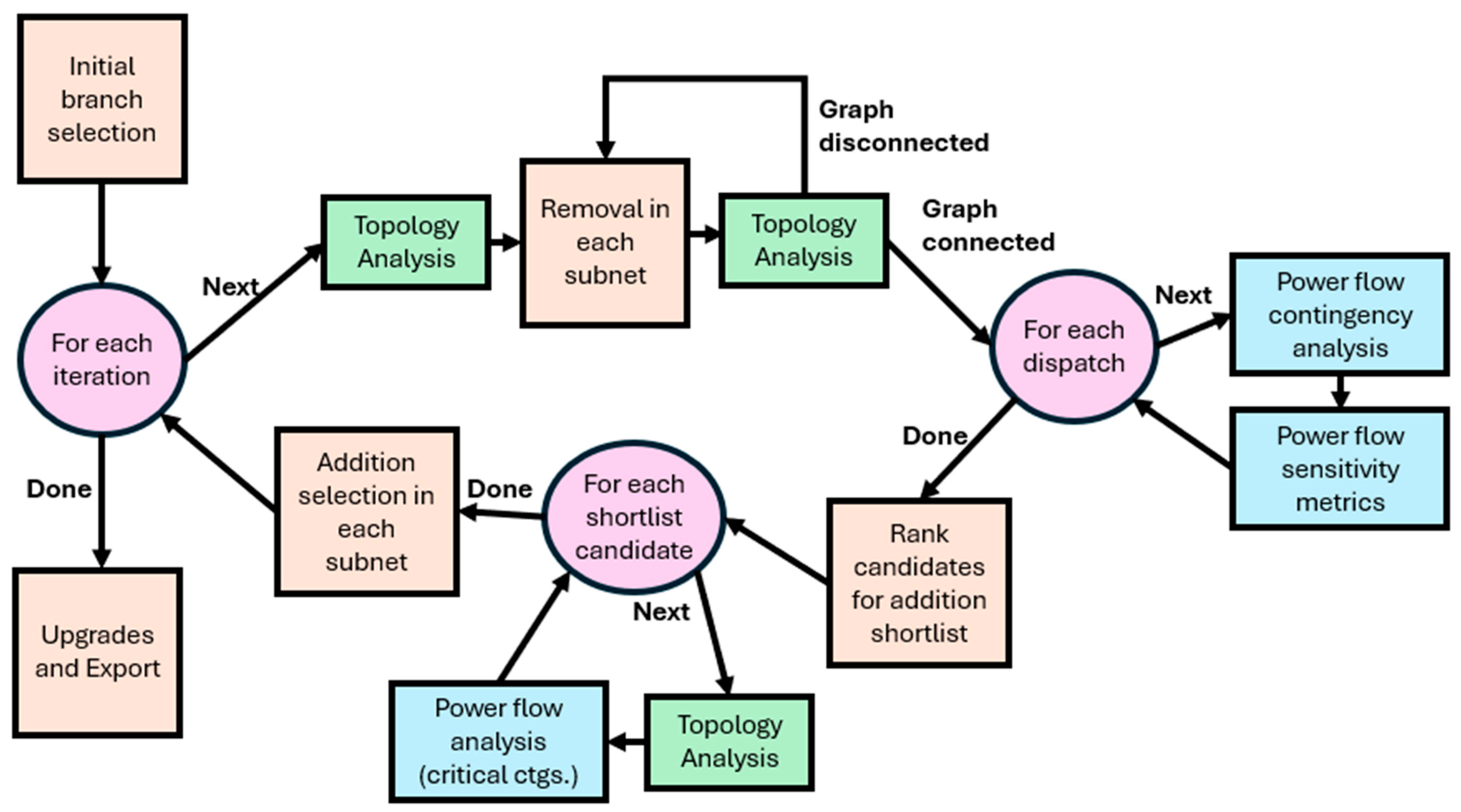
2.3. Solution Algorithm and Methodology for Network Expansion

This section gives the methodology followed for the solution of the TEP as proposed in this paper, with Figure 1 showing a flow chart of the algorithm. Below, each of the main boxes representing algorithm steps within the flow chart is explained in more detail.

Initial branch selection. The algorithm works on an iterative process that alternates between removal and addition. Therefore, the first step in this process is to do a preliminary selection of branches, i.e., the initial version of the vector $u$. Recall that the selection of $u$ only relates to the candidate lines for addition. The underlying grid that exists a priori is assumed to be in place, as represented by ${\mathcal{E}}_0$ (this is in contrast to the synthetic grid building process, in which no prior lines exist). There are two requirements on this selection for the algorithm, as formulated here. First, the graph $\mathcal{G}$ should be fully connected by its edge set $\mathcal{E}={\mathcal{E}}_{+}+{\mathcal{E}}_0$. This is required both to properly assess the topological constraints and to enable a convergent power flow solution. Second, the number of candidates selected (i.e., $\sum u$), must be equal to a predetermined number of branches to add. Since during the algorithm lines are added and removed in equal numbers, this initial decision is a parameter that can be tuned in an outer-loop iteration.

The following method is used to select $u$ initially for the purposes of this paper. First, add all branches of the substations’ Euclidean minimum spanning tree, which connect at least one new substation. This ensures the first requirement of a connected graph is met. Second, any additional branches can be added to meet the total requirement. We chose to select them uniformly at random from the first neighbors of the Delaunay triangulation to avoid starting with many extremely long lines.

Topology analysis. The second step to explain is the topology analysis subroutine, which is a core feature used in several places within the TEP solver. It performs two depth-first searches through the current selection of candidates (and prior branches) to collect three analyses: connectivity, bridge identification, and radial bus identification.

The first depth-first search traverses the full graph and determines two things: whether the graph is connected, as determined by whether every bus is reachable in the search, and which branches are “bridges” meaning they would separate the network. Branches can be shown to be bridges by keeping track of the lowest-rank bus that is reachable upstream of the branch, thus indicating any cycles the branch is part of. Branches that are part of a cycle cannot be bridges. Bridge identification is necessary because bridges correspond to contingencies that would isolate the system and preclude the solution of the contingency power flow with a single slack bus. Bridge identification is also necessary as a precursor to the third analysis, to identify radial buses, which are defined as buses that can be separated from the slack bus by the elimination of only one branch.

The second depth-first search identifies radial buses. This search is performed on the graph with bridges removed. Any bus not reachable in the search from the slack bus must be a radial bus. If the radial bus has any load, it will incur a penalty as defined in Equation (11).

Power flow contingency analysis. The third step for the algorithm, as shown in Figure 1, is the power flow contingency analysis. The power flow solution is solved as in Equation (7) for base and contingency conditions. As discussed above, the selection of $p$ in (7) for the generation and load profiles is an important consideration. The algorithm as described in Figure 1 allows for multiple dispatches (with two dispatches selected here). In contingency analysis with a large number of contingencies, the resulting outputs could potentially be large in terms of data volume. To address this, in line with the problem formulation, each branch retains only its maximum flow in any contingency, such that as each contingency is solved, it updates these values if the prior maximum is exceeded. A record is also kept of the contingency in which this maximum occurs.

Linearized, DC power flow solutions are used in this stage of the TEP solver for three reasons: (1) computational efficiency as opposed to an AC power flow solution, (2) difficulty in handling convergence and other aspects when not all reactive power resources have been determined yet, and (3) for the purposes of long-term transmission line planning, the primary consideration is in the flow of active (real) power.

Power flow sensitivity analysis. The fourth step to explain is the sensitivity metric calculation. This is important to the targeted addition step as it allows the prioritization of branches that would reduce contingency overloads. Line innage sensitivities were first applied to the creation of synthetic electric grids in [5], and here they were likewise applied to the TEP solution. These sensitivities are formulated as follows:

$${\displaystyle \frac{\partial {\varphi }_k}{\partial B_i}}=-{\varphi }_i{e}_i^T{B}^{-1}{e}_k,$$

(14)

where $\varphi$ represents the bus voltage angle difference, $e$ is the zero vector with +1 and −1 in the buses associated with a right-of-way, and rights-of-way $i$ and $k$ are the candidate and overload branches, respectively. Hence, once the sensitivity vector $B^{-1}{e}_k$ is calculated once for the most critical overload that is to be targeted, any number of candidate lines $i$ can have their impacts on that overload estimated with simply three floating point operations: a subtraction of angles to get ${\varphi }_i$, a subtraction of two elements of the sensitivity vector to get $e_i^T{B}^{-1}{e}_k$, and one multiplication to get the final sensitivity. The application of this sensitivity to the TEP problem is, first, through selecting the set of the most severe contingency overloads, and second, through calculating (via (14)) and recording each candidate branch’s most significant sensitivity toward reducing (or intensifying, if negative) that overload.

Subnet definition. For the purposes of this algorithm, the network being designed is divided into geographic areas, and each voltage level within an area is considered a subdivision of the overall grid, or a “subnet”. While the topological and power flow contingency analyses are performed at a full system level, subnets are used for the actual removal and addition decisions as described in this and the next two paragraphs. This allows a degree of parallelization under the assumption that there is reduced impact between different subnets.

Removal in each subnet. The algorithm proceeds in iterations. At the beginning of each iteration, a topological analysis is performed, primarily to verify connectedness and identify bridges. Then, each subnet removes a single line (candidate lines only, not previously existing branches). Hence, removal is the fifth step to explain for this methodology. Two removal strategies are considered here, random and sequential. In both cases, the removal is not as a result of analysis but is designed to mimic, in the flavor of simulated annealing, minor disturbances to the network topology that will be addressed in the addition stage (in some cases, lines are removed that did not have much benefit to the system anyway, in which case there is nothing to fix; in other cases, the removed line may be immediately added back).

Random removal is performed uniformly, picking one of the currently selected candidate lines. Sequential removal keeps track of ordering candidates and removes them one by one. This allows quicker cycling through the consideration of all line removals. However, the intended effect is essentially the same—an arbitrary, slight perturbation to the network. One important restriction to note in the removal is that bridges may not be removed; the graph can never become disconnected.

In rare cases, the removal of two non-bridges by different subnets can together isolate the overall grid. To address this issue, during the second topological analysis (necessary anyway for labeling new bridges and radial nodes), if the graph is found to be disconnected, the removed lines are restored, and new removals are chosen.

Ranking candidates for the addition shortlist. The core idea of the algorithm is randomized removal followed by targeted addition. The approach is motivated by common heuristics such as simulated annealing, which approaches large, difficult discrete problems with a balance of a stochastic process (randomized change) and a gradient-based process (targeted change). By slowly moving from more randomized changes to more targeted changes, the heuristic enables the solution to consider more possibilities and avoid getting stuck via more greedy approaches.

The addition part of the process is the sixth step. Following the topological analysis, it is fairly straightforward to approximate the impact any candidate may have on the radial load penalties. From the power flow contingency analysis followed by sensitivity calculations, it is possible to estimate the relative impact each candidate may have on significant contributions to the branch overload penalty.

Unfortunately, what is not easy to determine is the relative weighting that should be given to fixed cost and overload components of a candidate’s expected impacts, since the overload sensitivity indicates mainly the relative, rather than actual, power increases. To address this and to allow for a more targeted addition selection, the algorithm proceeds with selecting an addition shortlist for each subnet. This shortlist contains, in the example of this paper, 10 candidates. These are selected as (1) the removed line, which should be considered for restoration; (2–4) the three lowest fixed-cost candidates that connect directly to significant radial loads; (5–9) the lowest cost candidate, with the cost determined by the fixed cost plus the overload sensitivity scaled by five different ratios (${10}^{-4},{10}^{-2},{10}^0,{10}^2, {10}^4$). The rest of the shortlist candidates are randomly selected from the available candidates (at least one but may be more if the candidates in (1–9) have duplicates). These shortlists are shuffled into a randomized order for iterative, detailed analysis again.

Addition selection in each subnet. For 10 iterations (one for each item in each subnet’s shortlist), the topological and power flow analyses are repeated with the shortlist candidate added. The power flow analysis is shortened by focusing only on the critical contingencies—the ones that resulted in significant overloads in the original, full contingency set analysis. A very close approximation of the actual objective value of the network can now be determined for each shortlist candidate. The only inaccuracies are due to, first, interference between subnet candidates, and second, the reduced contingency set. Each subnet then simply picks the shortlist candidate that had the most positive impact on the objective.

Termination conditions, final upgrades, and exports. The iterations can continue as long as desired, with a recommended number of iterations 5–10 times the number of candidate branches to add. In practice, the process is limited by computation time, stopping after a designated wall clock period. Once the iterations are complete, the final network is exported. Optionally, there is an upgrade routine as well to address minor branch overloads by adjusting the assumed line design (and, hence, the limit).

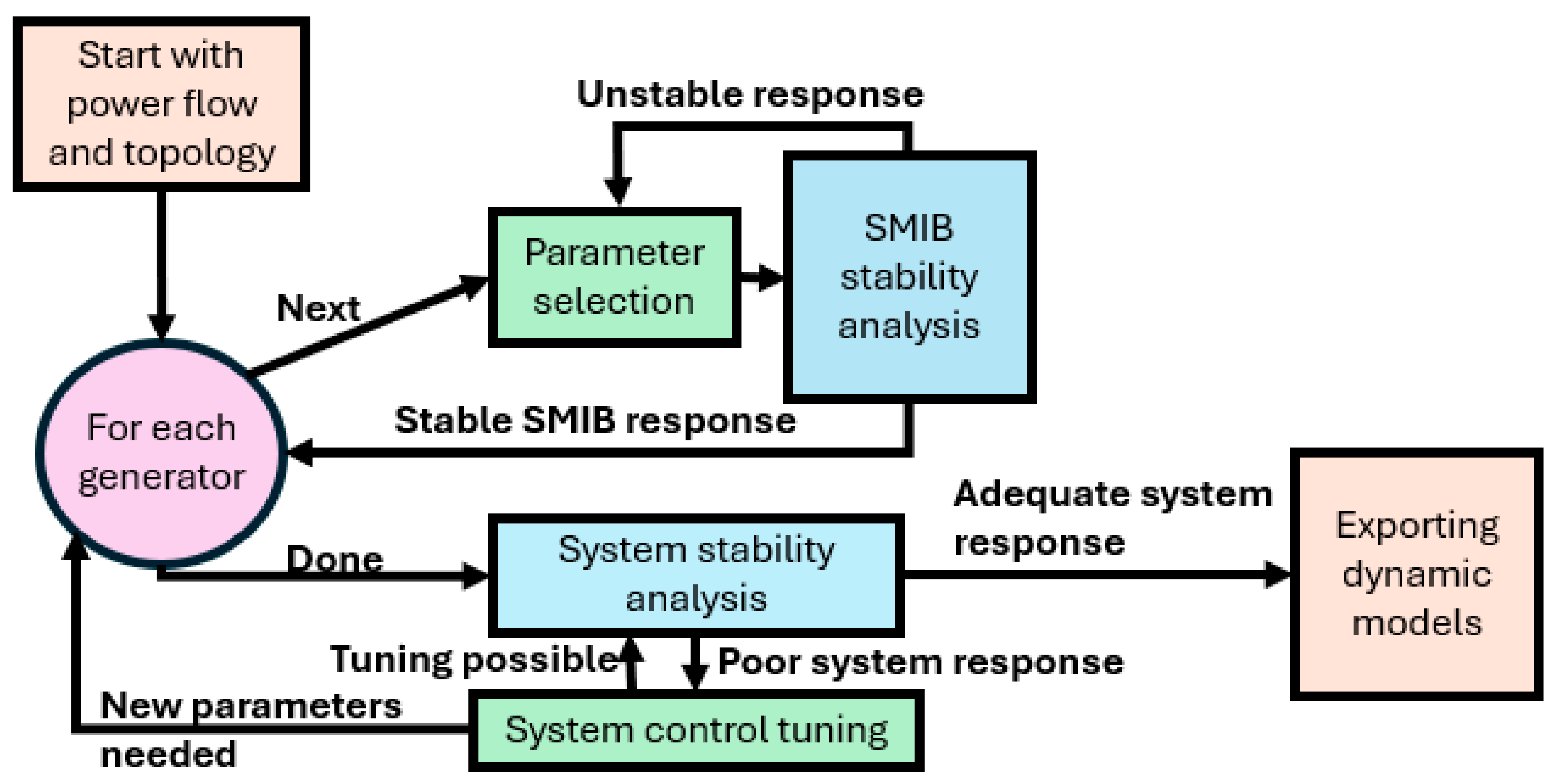
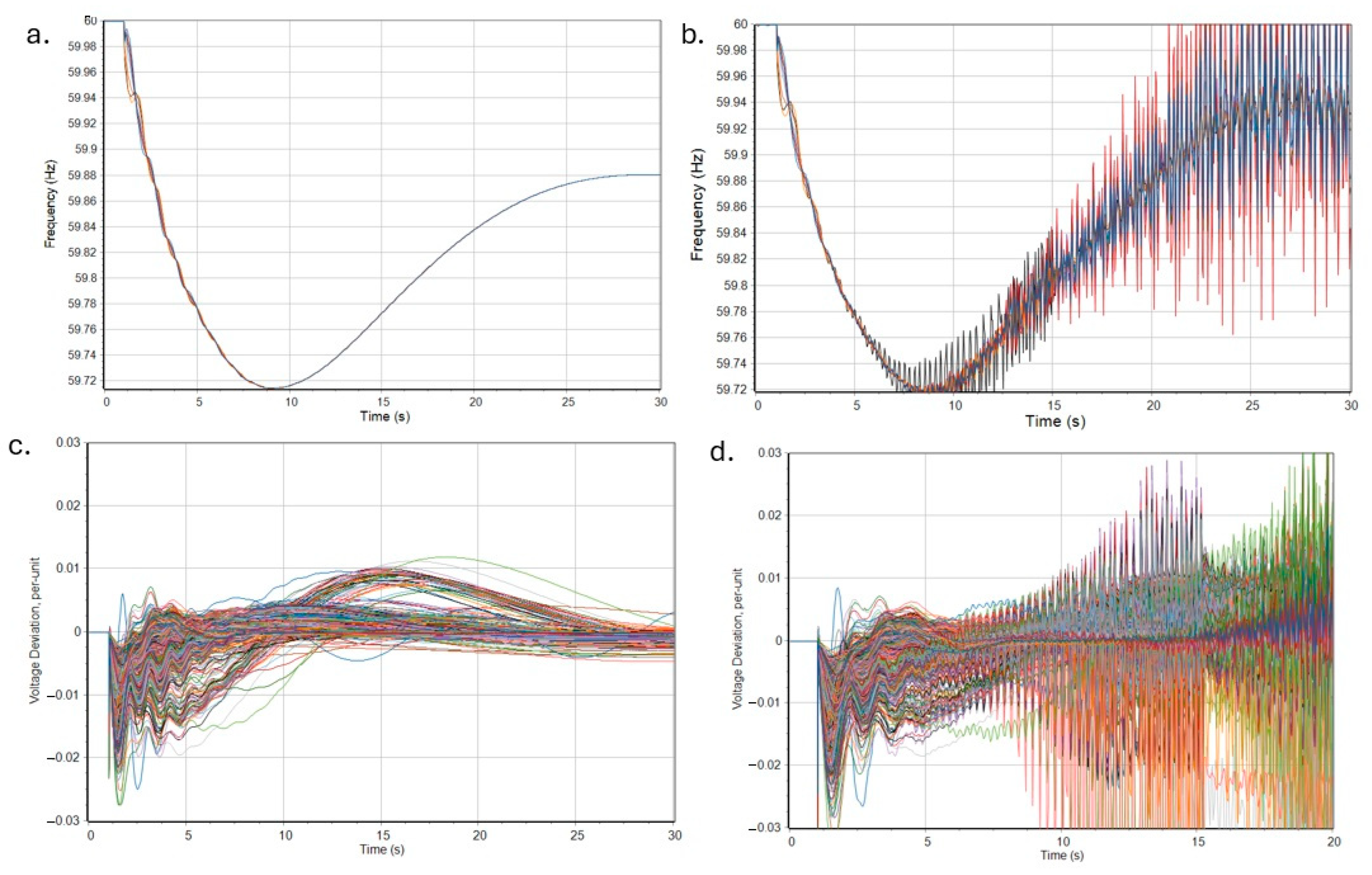
2.4. Design and Validation of Network Impacts on System Dynamics

As part of the network design and validation, this paper also describes the impact beyond real power steady-state flows (as determined from the base and contingency power flow) to consider impacts of voltage, rotor angle, and frequency controls. This effort is based on preliminary methodologies described in [44,45]. Prior to creating dynamic stability models, an AC power flow solution is found by adding appropriate reactive power resources.

The overall process is shown in Figure 2. For each generator, based on the fuel type, MW capacity, and statistics collected from actual cases, model types are assigned, along with parameters. Then, each generator (whether synchronous machine or inverter-based) is tested with single-machine, infinite-bus analysis to determine if the device-level response is adequate. If not, the parameter selection is repeated. Once all models have been assigned, system stability analysis is completed, modified by system control tuning methods. In some cases, the system performance cannot be adequately corrected by system control tuning, so the full parameter selection is repeated. However, normally, adequate system response can be quickly achieved.

The application of this process to the TEP solution design and validation will be demonstrated in the test case in the next section. The idea is that in the oscillation analysis of system dynamics, the extent to which the designed network produces a strong coherence among control systems throughout the grid could be identified. From here, specific topological results can be used to determine the extent to which power system inter-area oscillatory modes are affected by the transmission expansion.

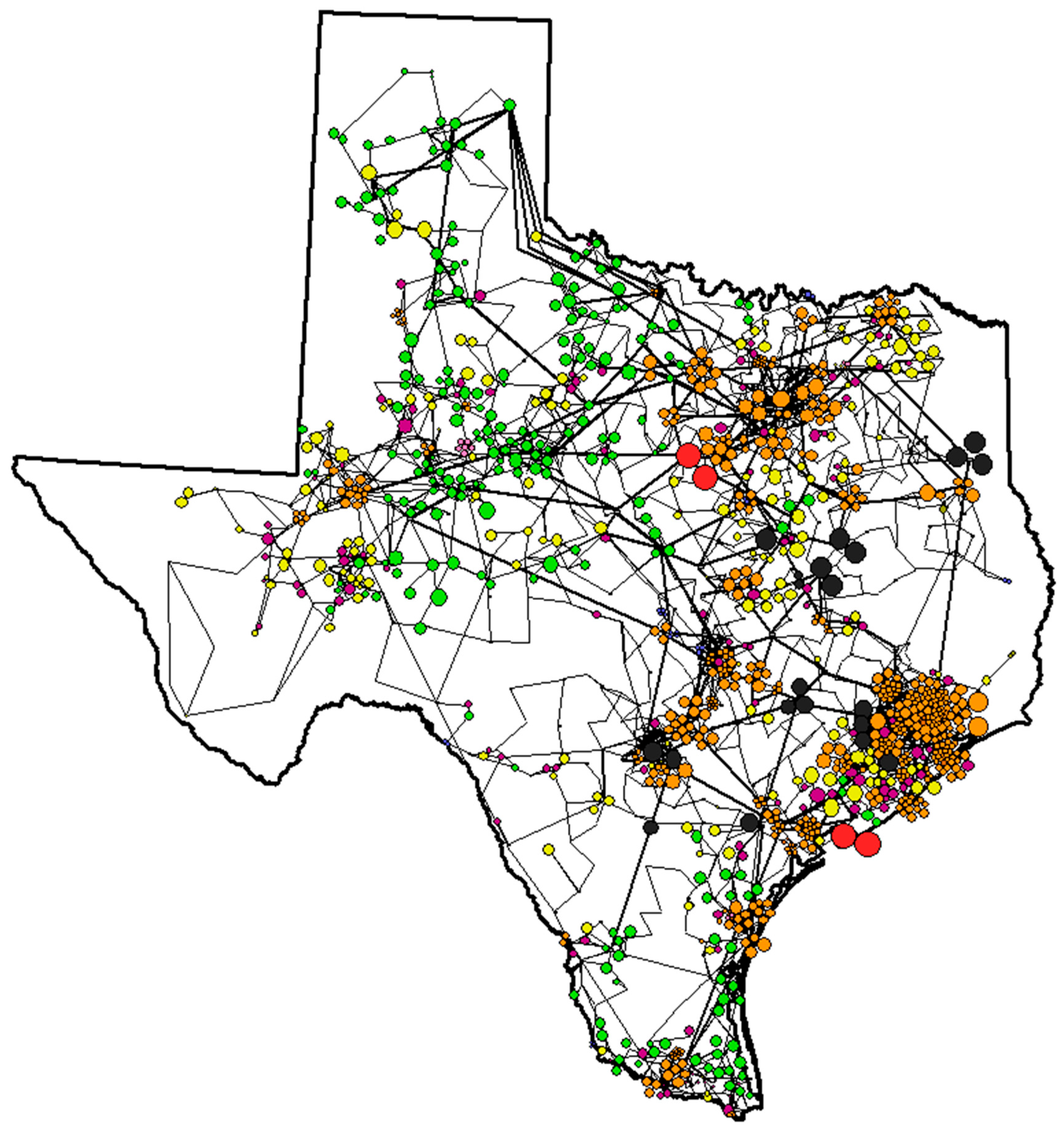
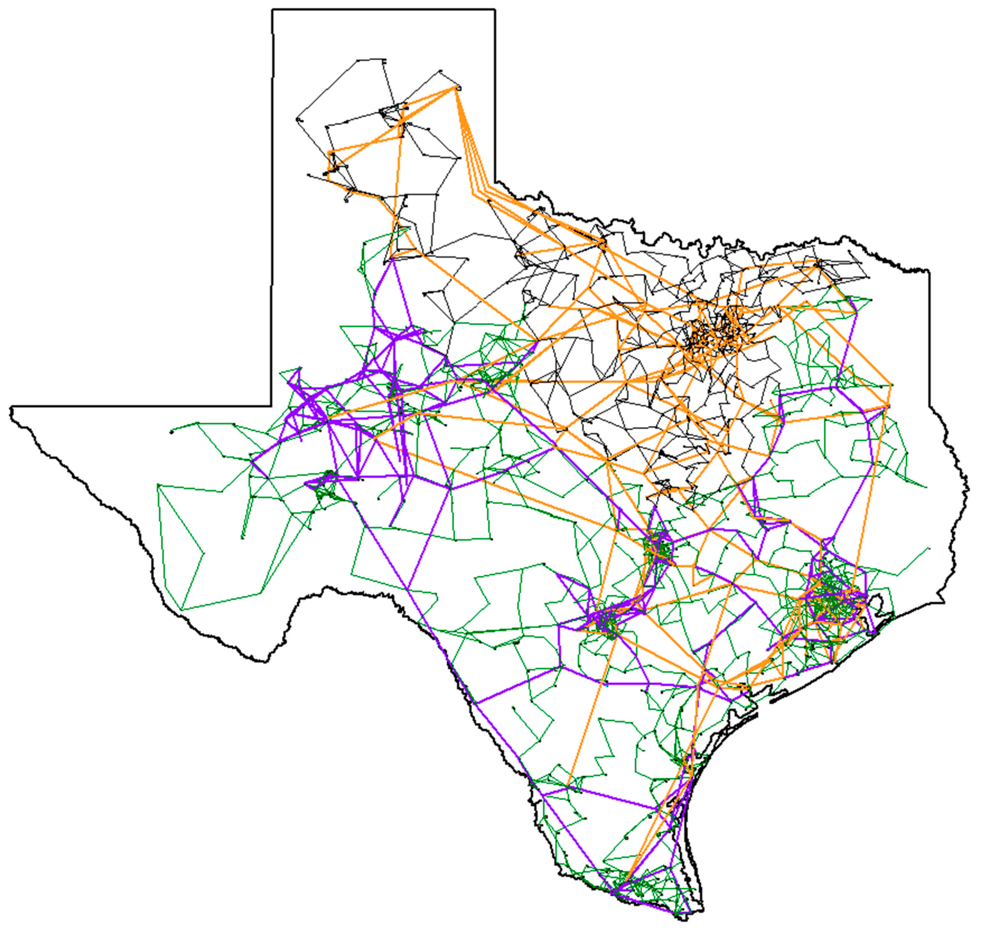
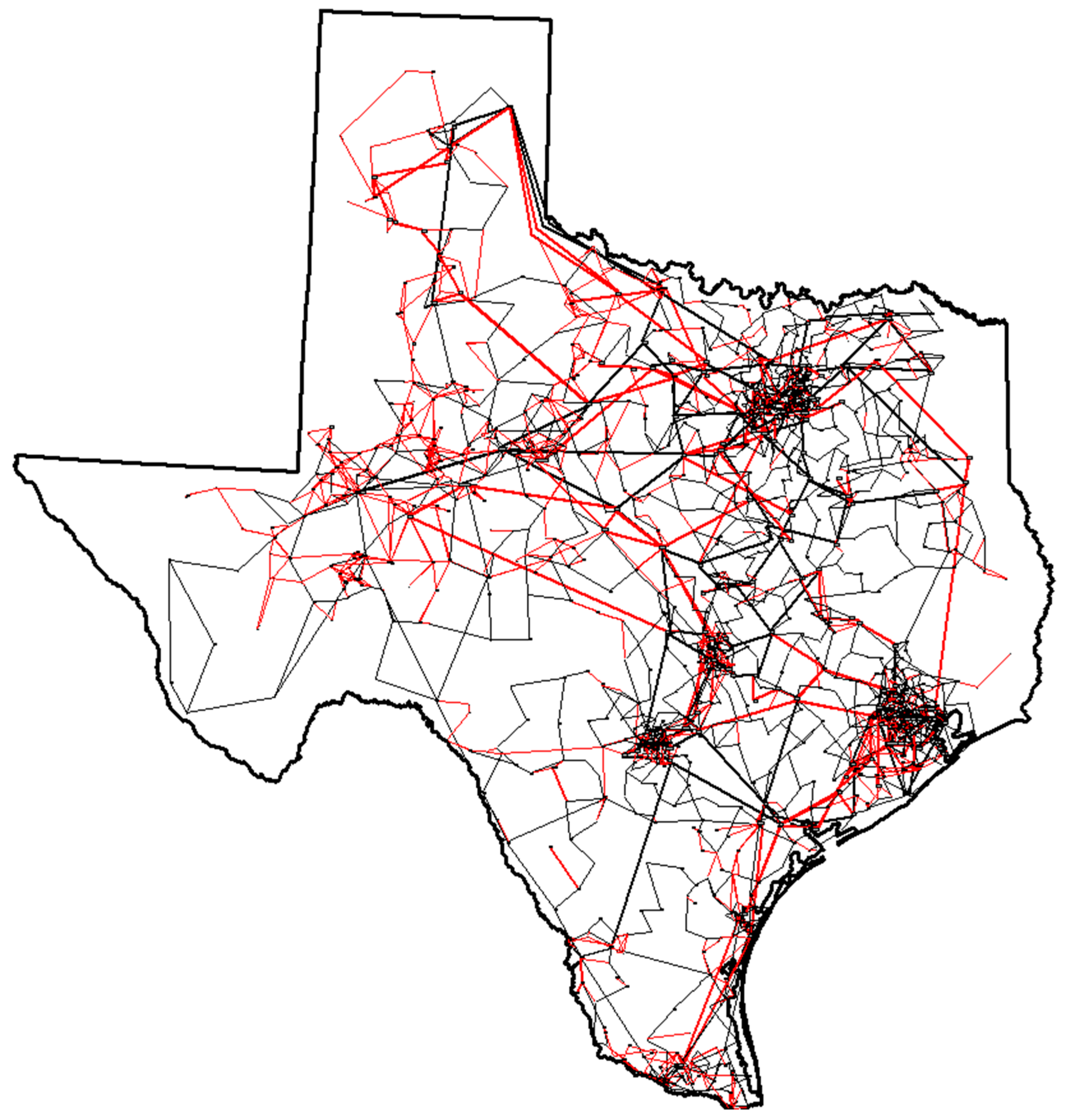
3. Case Study: Texas2k Synthetic Grid

This section presents a test case demonstrating the methodology of the paper on a large-scale system. The Texas2k electric grid is a synthetic test case, which is geographically based and does not represent any actual grid. It has 2000 buses and was first created in 2016, matching load and generation in the US state of Texas at that time [4].

The case study described here involves expanding that grid to consider the growth in load and generation (and the necessary corresponding growth in transmission infrastructure) between 2016 and 2025. This section describes the setup of the problem with load, generation, and transmission candidates, the solution to the problem with the proposed algorithm, and analysis and discussion of the solution, including impacts on dynamic performance.

The baseline of the problem is the 2016 Texas2k case (which is alternatively known as the ACTIVSg2000 case). This case has 67,109 MW of load and 100,085 MW of generation capacity. These represent the values of the Texas Interconnect load and generation at that time. As of 2025, the estimated peak load is 85,759 MW, and the estimated generation capacity is 166,481 MW in Texas Interconnect [46,47]. Therefore, to start, the case was revised to add appropriate load and generation.

Load. Public data are available on a weather-zone basis (8 weather zones in the case) for the load increase [46]. Each zone’s loads were increased using a stochastic selection to match the new designed total. This process, using the existing load objects, worked well for all zones except the “Far West” zone, which had such a large load increase that many new loads were needed, primarily due to significant new demand growth in this region of Texas. Twenty new load substations were created in randomized locations within this region and assigned loads of varying values around 150 MW. In total, the new load summed to the correct value of 85,759 MW, with each zone accounted for correctly.

Generation. The US Energy Information Administration (EIA) requires Form-860 data to be filed annually for medium-to-large electric generating stations in the US. These EIA data are publicly available and provide generator fuel types, maximum MW capacity, and geographic location, among other generator details. These data were used in [4] in its 2016 form for building the synthetic Texas2k case’s original generation fleet. Likewise, for this case study, the 2025 EIA 860 data were used to add new generators to the case, such that the final set of generators in the case matched all in-service generators as of 2024 as well as the anticipated new installations in 2025. This involved removing some prior generators that were either retired or had data errors in the original case. It also involved adding new substations for new generating plants, and adding generating units to some original plants.

Table 2. New generation totals in the 2025 Texas2k grid, along with commitment and dispatch decisions for the planning case scenario used in the TEP solution.

All Values in MW	Installed	Committed	Dispatched	Committed Percentage	Dispatch Percentage
BIT (bituminous coal)	13,538	11,688	4145	86%	35%
DFO (distillate fuel oil)	514	406	170	79%	42%
MWH (energy storage)	14,277	7304	7304	51%	100%
NG (natural gas)	58,087	29,164	19,496	50%	67%
NUC (nuclear)	4980	4980	4775	100%	96%
OBL (other biomass liquids)	160	142	142	89%	100%
OTH (other)	228	138	138	61%	100%
SUN (solar)	32,313	21,120	21,120	65%	100%
WAT (water)	552	480	480	87%	100%
WND (wind)	41,832	32,534	32,534	78%	100%
Total	166,481	107,956	90,304	65%	84%

shows the generation totals used in the 2025 grid, and these new generators are shown in Figure 3.

New substations and buses. The original case had 1250 substations and 2000 buses. There was a need for 304 new substations to be created to accommodate the new generation plants, along with the new load in the Far West region. The main transmission levels in the case were 115 kV and 161 kV, determined by area. In addition to adding one bus at this level for each of the new substations, new buses were needed for the low side of the generator step-up transformers. Furthermore, new buses were added at the 230 kV and 500 kV levels for new, larger generators and large load increases. In total, 789 new buses were created, bringing the system total to 1554 substations and 2789 buses. These new substations and buses, before any additional transmission was added, were not connected into the grid.

Transmission line candidates. The transmission line candidate creation process used the third neighbors of the Delaunay triangulation to produce a raw list of 40,659 candidate transmission lines. Based on the length of line, scaled by some geographic features, the fixed costs of the lines (in scaled kilometers) ranged from 0.22 to 184,912, with 90% of the candidate lines falling in the range of 10 to 1000. The lines were assigned impedances and limits associated with their voltage levels and length.

TEP solution. The proposed TEP solution algorithm was run for a period of 18 h, consisting of about 4000 iterations of the stochastic removal, targeted addition actions. The lowest objective incumbent solution was then selected for final upgrade analysis.

Figure 4 shows the new transmission network after the TEP solution is complete, demonstrating visually the network expansion areas and levels. The top figure shows the transmission network, color-coded by nominal voltage level. The bottom figure shows the lines, with newly added transmission lines colored red. The figure in particular shows a match between the areas of new generation and load and the areas where new transmission is concentrated. As can be seen from the figure, new transmission is concentrated in the western part of the grid, where tremendous growth in new load and generation took place, and in the Gulf Coast area south of Houston, where there is a significant new solar station. There were also additional new transmission facilities needed throughout the case to accommodate new load and generation.

Table 3. Objective values for the TEP solution on the Texas2k case study.

Objective Value	${\mathit{z}}_{\mathit{f}}$	${\mathit{z}}_{\mathit{r}}$	${\mathit{z}}_{\mathit{c}}$	$\mathit{z}$
Initial	70,181	12,890	47,700	130,772
Final incumbent	55,361	2724	23,783	81,868

shows the objective values in both the initial and final incumbent networks for this TEP solution. The table also shows the objective value broken down into the components for the fixed cost ($z_c$), the radial load ($z_r$), and the contingency overload ($z_c$). As can be seen in the table, the TEP solver was successful in reducing all three categories of objectives significantly, for a problem that would be too large (with over 40,000 candidates and 3000 contingencies) for a direct integer programming-based method. This shows the benefit of the proposed method and its effectiveness in addressing the problem.

The final grid model was released online in [48] in a variety of common industry formats, as well as the TEP problem data to allow benchmarking. The dataset download includes the original 2016 case, the case with only new substations, load, and generation added, as well as a spreadsheet list of the candidate transmission lines considered.

Results with dynamic grid modeling. After completion of the TEP, new grid dynamics models were generated. A frequency response study was then run on the resulting grid by removing the two largest generating units and simulating the effect of the network’s inertial response and primary frequency response, both from synchronous machines and inverter-based resources (IBRs). The results are shown in the top plot of Figure 5. The new transmission network’s strength is crucial to ensuring a unified frequency response with good generator coherence and well-damped oscillations. For comparison, the bottom plot in Figure 5 shows an unstable response resulting from a weaker network, created by increasing the reactance of the newly added transmission branches in the system by 20%. In addition, Figure 5 shows voltage traces between the final incumbent network and, for comparison, a weaker network.

This instability can be quantified with iterative matrix pencil modal analysis by noting that modal decomposition of the voltage response from the final incumbent network had no modes from 0.01 to 10 Hz with low or negative damping, whereas the modal analysis of the voltage response from the weaker network (Figure 5d) identified no fewer than 77 negatively damped modes in the 0.01 to 10 Hz range.

4. Conclusions

This paper introduces a methodology based on network synthesis methods for approaching very large-scale TEP problems. The methods, originally designed for creating synthetic electric grid models, use an iterative approach with stochastic removal and targeted addition. The core optimization objectives seek to balance fixed costs against grid strength characteristics, such as by removing the radial load and reducing the branch overloads in single-element outage contingency power flows. The methodology is demonstrated on the Texas2k synthetic network, expanded from its original 2016 scope to new load and generation in 2025. The methodology is shown to produce a viable new expansion to the network with a reduced cost and low contingency violations.

A secondary analysis, supplemental to the main analysis, is enabled by the ability to add transient stability models to the new generators. This dynamic analysis allows for examining the impact of the network on generator synchronism, showing that the produced network, which was formed with primary objectives of static contingency robustness, topology, and investment cost, has a stable response even for a very large frequency event.

The value of this paper’s contribution is in demonstrating a novel, heuristic-based approach to the TEP problem that shows promise for a realistic TEP solver that balances many design criteria at a scale not feasible for the existing integer programming-based methods. This method is demonstrated on a large-scale synthetic test case. Prior efforts on the TEP problem have largely focused on direct, integer programming-based methods, which have inherent scalability challenges. Interesting directions for future work include expanding the analysis to AC power flow studies, additional dispatch scenarios, along with theoretical and experimental comparison with integer programming-based methods. Further improvements on the proposed method would also include exploring the effects of parameters such as optimization cost coefficients and ranking weights and tuning them for optimal performance. With the tremendous growth in load and renewable generation resources, as electric utilities look into long-term future planning scenarios, the need for more efficient, higher-scaling expansion planning solutions such as the one proposed here will be essential.

References

1. U.S. Department of Energy. National Transmission Needs Study. 2023. Available online: https://www.energy.gov/gdo/national-transmission-needs-study (accessed on 15 July 2025).
2. Electric Reliability Council of Texas (ERCOT). 2024 Regional Transmission Plan (RTP) 345-kV Plan and Texas 765-kV Strategic Transmission Expansion Plan Comparison. 2025. Available online: https://www.ercot.com/files/docs/2025/01/27/2024-regional-transmission-plan-rtp-345-kv-plan-and-texas-765-kv-strategic-transmission-expans.pdf (accessed on 15 July 2025).
3. Clean Energy Finance Corporation (CEFC). CEFC Annual Report 2023–2024. 2024. Available online: https://www.cefc.com.au/document?file=/media/d3dodzn3/cefc_annualreport2023-24.pdf (accessed on 15 July 2025).
4. Birchfield, A.B.; Xu, T.; Gegner, K.M.; Shetye, K.S.; Overbye, T.J. Grid structural characteristics as validation criteria for synthetic networks. IEEE Trans. Power Syst. 2017, 32, 3258–3265. [Google Scholar] [CrossRef]
5. Birchfield, A.B.; Overbye, T.J. Planning sensitivities for building contingency robustness and graph properties into large synthetic grids. In Proceedings of the Hawaii International Conference on System Sciences, Maui, HI, USA, 7–10 January 2020; pp. 1–8. [Google Scholar]
6. Latorre, G.; Cruz, R.D.; Areiza, J.M.; Villegas, A. Classification of publications and models on transmission expansion planning. IEEE Trans. Power Syst. 2003, 18, 938–946. [Google Scholar] [CrossRef]
7. Mahdavi, M.; Antunez, C.S.; Ajalli, M.; Romero, R. Transmission Expansion Planning: Literature Review and Classification. IEEE Syst. J. 2019, 13, 3129–3140. [Google Scholar] [CrossRef]
8. Zhang, H.; Vittal, V.; Heydt, G.T.; Quintero, J. A mixed-integer linear programming approach for multi-stage security-constrained transmission expansion planning. IEEE Trans. Power Syst. 2012, 27, 1125–1133. [Google Scholar] [CrossRef]
9. Zhang, F.; Hu, Z.; Song, Y. Mixed-integer linear model for transmission expansion planning with line losses and energy storage systems. IET Gener. Transm. Distrib. 2013, 7, 919–928. [Google Scholar] [CrossRef]
10. Pozo, D.; Sauma, E.E.; Contreras, J. A three-level static MILP model for generation and transmission expansion planning. IEEE Trans. Power Syst. 2013, 28, 202–210. [Google Scholar] [CrossRef]
11. Aghaei, J.; Amjady, N.; Baharvandi, A.; Akbari, M.A. Generation and transmission expansion planning: MILP–based probabilistic model. IEEE Trans. Power Syst. 2014, 49, 1592–1601. [Google Scholar] [CrossRef]
12. Camponogara, E.; de Almeida, K.C.; Junior, R.H. Piecewise-linear approximations for a non-linear transmission expansion planning problem. IET Gener. Transm. Distrib. 2015, 9, 1235–1244. [Google Scholar] [CrossRef]
13. Zhan, J.; Chung, C.Y.; Zare, A. A fast solution method for stochastic transmission expansion planning. IEEE Trans. Power Syst. 2017, 32, 4684–4695. [Google Scholar] [CrossRef]
14. Huang, S.; Dinavahi, V. A branch-and-cut benders decomposition algorithm for transmission expansion planning. IEEE Syst. J. 2019, 13, 659–669. [Google Scholar] [CrossRef]
15. Majidi-Qadikolai, M.; Baldick, R. A generalized decomposition framework for large-scale transmission expansion planning. IEEE Trans. Power Syst. 2018, 33, 1635–1649. [Google Scholar] [CrossRef]
16. Akbari, T.; Bina, M.T. Approximated MILP model for ac transmission expansion planning: Global solutions versus local solutions. IET Gener. Transm. Distrib. 2016, 10, 1563–1569. [Google Scholar] [CrossRef]
17. Rahmani, M.; Romero, R.A.; Rider, M.J. Risk/investment-driven transmission expansion planning with multiple scenarios. IET Gener. Transm. Distrib. 2013, 7, 154–165. [Google Scholar] [CrossRef]
18. García-Bertrand, R.; Mínguez, R. Dynamic robust transmission expansion planning. IEEE Trans. Power Syst. 2017, 32, 2618–2628. [Google Scholar] [CrossRef]
19. Orfanos, G.A.; Georgilakis, P.; Hatziargyriou, N.D. Transmission expansion planning of systems with increasing wind power integration. IEEE Trans. Power Syst. 2013, 28, 1355–1362. [Google Scholar] [CrossRef]
20. Mínguez, R.; García-Bertrand, R.; Arroyo, J.M.; Alguacil, N. On the solution of large-scale robust transmission network expansion planning under uncertain demand and generation capacity. IEEE Trans. Power Syst. 2018, 33, 1242–1251. [Google Scholar] [CrossRef]
21. Bolgaryn, R.; Wang, Z.; Scheidler, A.; Braun, M. Active power curtailment in power system planning. IEEE Open Access J. Power Energy 2021, 8, 399–408. [Google Scholar] [CrossRef]
22. Peng, L.; Zabihi, A.; Azimian, M.; Shirvani, H.; Shahnia, F. Developing a robust expansion planning approach for transmission networks and privately-owned renewable sources. IEEE Access 2023, 11, 76046–76058. [Google Scholar] [CrossRef]
23. Dehghan, S.; Amjady, N.; Conejo, A.J. Reliability-constrained robust power system expansion planning. IEEE Trans. Power Syst. 2016, 31, 2383–2392. [Google Scholar] [CrossRef]
24. Moreira, A.; Street, A.; Arroyo, J.M. An adjustable robust optimization approach for contingency-constrained transmission expansion planning. IEEE Trans. Power Syst. 2015, 30, 2013–2022. [Google Scholar] [CrossRef]
25. Shortle, J.; Rebennack, S.; Glover, F.W. Transmission-capacity expansion for minimizing blackout probabilities. IEEE Trans. Power Syst. 2014, 29, 43–52. [Google Scholar] [CrossRef]
26. Zhang, X.; Tomsovic, K. Security constrained multi-stage transmission expansion planning considering a continuously variable series reactor. IEEE Trans. Power Syst. 2017, 32, 4442–4450. [Google Scholar] [CrossRef]
27. Meneses, M.; Nascimento, E.; Macedo, L.H.; Romero, R. Transmission network expansion planning considering line switching. IEEE Access 2020, 8, 115148–115158. [Google Scholar] [CrossRef]
28. da Silva, A.M.L.; Rezende, L.S.; Honorio, L.M.; Manso, L.A.F. Performance comparison of metaheuristics to solve the multi-stage transmission expansion planning problem. IET Gener. Transm. Distrib. 2011, 5, 360–367. [Google Scholar] [CrossRef]
29. Gallego, R.A.; Alves, A.B.; Monticelli, A.; Romero, R. Parallel simulated annealing applied to long term transmission network expansion planning. IEEE Trans. Power Syst. 1997, 12, 181–188. [Google Scholar] [CrossRef]
30. Murugan, P. Modified particle swarm optimisation with a novel initialisation for finding optimal solution to the transmission expansion planning problem. IET Gener. Transm. Distrib. 2012, 6, 1132–1142. [Google Scholar] [CrossRef]
31. Huang, S.; Dinavahi, V. Multi-group particle swarm optimisation for transmission expansion planning solution based on LU decomposition. IET Gener. Transm. Distrib. 2017, 11, 1434–1442. [Google Scholar] [CrossRef]
32. Mahdavi, M.; Kimiyaghalam, A.; Alhelou, H.H.; Javadi, M.S.; Ashouri, A.; Catalão, J.P.S. Transmission expansion planning considering power losses, expansion of substations and uncertainty in fuel price using discrete artificial bee colony algorithm. IEEE Access 2021, 9, 135983–135995. [Google Scholar] [CrossRef]
33. Alhamrouni, I.; Khairuddin, A.; Ferdavani, A.K.; Salem, M. Transmission expansion planning using AC-based differential evolution algorithm. IET Gener. Transm. Distrib. 2014, 8, 1637–1644. [Google Scholar] [CrossRef]
34. Barati, F.; Seifi, H.; Sepasian, M.S.; Nateghi, A.; Shafie-khah, M.; Catalao, J.P.S. Multi-period integrated framework of generation, transmission, and natural gas grid expansion planning for large-scale systems. IEEE Trans. Power Syst. 2015, 30, 2527–2537. [Google Scholar] [CrossRef]
35. Moradi, M.; Abdi, H.; Lumbreras, S.; Ramos, A.; Karimi, S. Transmission expansion planning in the presence of wind farms with a mixed AC and DC power flow model using an imperialist competitive algorithm. Elect. Power Syst. Res. 2016, 140, 493–506. [Google Scholar] [CrossRef]
36. Rawa, M. Towards avoiding cascading failures in transmission expansion planning of modern active power systems using hybrid snake-sine cosine optimization algorithm. Mathematics 2022, 10, 1323. [Google Scholar] [CrossRef]
37. Zoppei, R.T.; Delgado, M.A.J.; Macedo, L.H.; Rider, M.J.; Romero, R. A branch and bound algorithm for transmission network expansion planning using nonconvex mixed-integer nonlinear programming models. IEEE Access 2022, 10, 39875–39888. [Google Scholar] [CrossRef]
38. Liu, G.; Sasaki, H.; Yorino, N. Application of network topology to long range composite expansion planning of generation and transmission lines. Elect. Power Syst. Res. 2001, 57, 157–162. [Google Scholar] [CrossRef]
39. Armaghani, S.; Naghshbandy, A.H.; Shahrtash, S.M. A novel multi-stage adaptive transmission network expansion planning to countermeasure cascading failure occurrence. Electr. Power Energy Syst. 2020, 115, 105415. [Google Scholar] [CrossRef]
40. Yang, Q.; Wang, J.; Zhang, Y.; Li, Q. A network search space reduction method for robust coordinated energy storage and transmission expansion planning. IET Gener. Transm. Distrib. 2024, 18, 1449–1465. [Google Scholar] [CrossRef]
41. Soltan, S.; Zussman, G. Generation of synthetic spatially embedded power grid networks. In Proceedings of the 2016 IEEE Power and Energy Society General Meeting (PESGM), Boston, MA, USA, 19 July 2016; pp. 1–5. [Google Scholar]
42. Espejo, R.; Lumbreras, S.; Ramos, A. A Complex-Network Approach to the Generation of Synthetic Power Transmission Networks. IEEE Syst. J. 2019, 13, 3050–3058. [Google Scholar] [CrossRef]
43. Birchfield, A.B.; Schweitzer, E.; Athari, M.H.; Xu, T.; Overbye, T.J.; Scaglione, A.; Wang, Z. A metric-based validation process to assess the realism of synthetic power grids. Energies 2017, 10, 1233. [Google Scholar] [CrossRef]
44. Xu, T.; Birchfield, A.B.; Overbye, T.J. Modeling, tuning, and validating system dynamics in synthetic electric grids. IEEE Trans. Power Syst. 2018, 33, 6501–6509. [Google Scholar] [CrossRef]
45. Baek, J.; Birchfield, A.B. A tuning method for exciters and governors in realistic synthetic grids with dynamics. In Proceedings of the 2023 North American Power Symposium (NAPS), Asheville, NC, USA, 15–17 October 2023; pp. 1–6. [Google Scholar]
46. ERCOT. 2025 ERCOT System Planning Long-Term Hourly Peak Demand and Energy Forecast. 2025. Available online: https://www.ercot.com/files/docs/2025/04/08/2025-LTLF-Report.pdf (accessed on 15 July 2025).
47. U.S. Energy Information Association, Form EIA-860. 2024. Available online: http://www.eia.gov/electricity/data/eia860/ (accessed on 15 July 2025).
48. Texas A&M University Electric Grid Test Case Repository. Available online: https://electricgrids.engr.tamu.edu/texas2k-series25/ (accessed on 15 July 2025).
Figure 1. Flow chart of the solution algorithm for network expansion.
Energies 18 03844 g001
Figure 2. Flow chart of dynamic model selection (see [45] for more details). SMIB refers to single-machine, infinite-bus (SMIB) stability analysis.
Energies 18 03844 g002
Figure 3. All generators, including new units, in the 2025 Texas2k grid. Red is nuclear, black is coal, orange is natural gas, green is wind, yellow is solar, blue is hydro, and purple is battery storage. The size of each circle indicates the real power capacity of the generator.
Energies 18 03844 g003
Figure 4. New transmission in the Texas 2k case. Top: colored by voltage level. Orange is 500 kV, purple is 230 kV, green is 161 and 115 kV. Bottom: new lines shown in red.
Energies 18 03844 g004aEnergies 18 03844 g004b
Figure 5. Time-domain response plots for a dynamic model of the expanded Texas2k case. (a) Average bus frequency for each of the eight areas, stable response from the actual final incumbent solution network. (b) For comparison, the average bus frequency response for each of the eight areas, unstable response resulting from a weaker network, as exemplified by increasing the reactance of new branches by 20%. (c) Individual bus voltage deviation response, stable response from the actual final incumbent solution network. (d) For comparison, individual bus voltage deviation response for each of the eight areas, unstable response resulting from a weaker network.
Energies 18 03844 g005