Multi-Objective Sensitivity Analysis of Hydraulic–Mechanical–Electrical Parameters for Hydropower System Transient Response

Abstract

Hydropower’s ability to start up and shut down quickly, combined with its flexible regulation characteristics, effectively alleviates frequency fluctuations caused by new energy sources, ensuring the safe and stable operation of the power system. However, during peak-frequency regulation tasks, the transition processes associated with the startup, shutdown, and load changes introduce frequent shocks to subsystems such as the hydro-turbine, governor, and diversion systems. These shocks pose significant challenges to the safe and stable operation of hydropower plants. Therefore, this study constructs a coupled hydraulic–mechanical–electrical model that incorporates the diversion system, hydro-turbine, governor, generator, and load, based on operational data from a real-world hydropower plant in China. The load increase transition process is selected for parameter sensitivity analysis to evaluate the influence of various structural, operational, and control parameters on unit stability and to identify key parameters affecting stability. The results indicate that the initial load exhibits the highest sensitivity to inversion power peak and rotational speed overshoot, with sensitivity values of 0.14 and 0.0038, respectively. The characteristic water head shows the greatest sensitivity to the inversion power peak time and rotational speed peak time, with values of 0.31 and 0.43, respectively. Additionally, the integration gain significantly influences the rotational speed rise time, with a sensitivity value of 0.30. These findings provide a theoretical basis for optimizing the parameter selection in hydropower plants.

1. Introduction

Hydropower is a crucial component of the future renewable energy mix, characterized by its clean, environmentally friendly nature, flexible scheduling, and low operating costs [1,2]. Developing the hydropower industry is essential for meeting the growing energy demand, optimizing the energy structure, conserving energy, reducing emissions, and ensuring the safety and stability of the power system [3,4]. With its ability to accurately track load changes and dynamically adjust, hydropower is the ideal energy source for regulating grid fluctuations, optimizing capacity allocation, and providing peak load support [5]. However, during frequent peak load and frequency regulation tasks, hydroelectric systems undergo transitional processes, such as startup, shutdown, and load adjustments [6]. In these processes, various system parameters continuously change and may even enter abnormal states. Prolonged operation under such conditions accelerates the degradation of core components, such as the rotor [7], posing significant risks to the safety and reliability of the hydropower station’s operation. Furthermore, since a hydropower system is a complex integration of hydraulic, mechanical, and electrical subsystems [8], it is essential to fully account for the interactions and coupling between these subsystems to accurately capture the dynamic response characteristics during transient processes. Therefore, constructing a simulation model that accurately reflects the dynamic response in the transient process and revealing the mechanism of structural design, operating conditions, and speed control parameters on the stability of the unit has become the key to ensuring the safe and stable operation of the hydropower system [9].

Currently, research on the operational stability of hydropower systems can be broadly categorized into two main areas: the development of power system models and the analysis of the influence of operational parameters. In terms of model development, relevant scholars commonly employ numerical simulation methods. Compared to conventional experimental measurements, numerical simulation effectively overcomes limitations in cost, time, and research depth [10]. This approach enables a comprehensive and accurate observation of physical phenomena and parameter variations at critical locations under extreme operating conditions through in-depth system analysis. These advantages are particularly pronounced in materials research, as clearly demonstrated in the studies by EL-SAPA et al. (2022, 2023, 2022) [11,12,13]. In the context of our research, Celebioglu et al. (2017) [14] employed the commercial software ANSYS Bladegen to investigate cavitation characteristics of hydroelectric units under off-design flow conditions, ultimately achieving cavitation-free operation optimization for an actual turbine runner. Yang et al. (2016) [15] conducted modeling using TOPSYS from a control perspective, investigating the wear mechanisms in hydropower units during primary frequency regulation, and identified effective methods to reduce wear. In mechanical systems, Valentín et al. (2017) [16] developed a hydraulic–mechanical–electrical coupled model using the finite element method to study the relationship between instability and power oscillations under partial load and overload conditions. Zhang et al. (2019) [17] expanded on previous work with a hydraulic–mechanical–electrical–structural model, exploring the vibration behavior of critical components such as guide bearings, rotors, and runners under sudden load increases.

Regarding the influence of parameters on unit operation, relevant scholars have conducted extensive research in three main areas: transient analysis and dynamic studies, optimization and structural analysis of hydraulic systems, and system stability and control strategy optimization. Ma et al. (2024) [18] proposed a framework for transient analysis under parameter uncertainty, encompassing integrated modeling, uncertain transient analysis, and transient calibration. Their findings highlighted the significant impact of six hydraulic generator parameters on transient characteristics, with casing pressure being particularly critical. Zhu et al. (2022) [19] employed trajectory sensitivity analysis to examine the sensitivity of the model’s state variables and their primary and secondary relationships to subsystem parameter changes. They demonstrated that state variables are highly sensitive to variations in the hydraulic turbine torque transfer coefficient, unit inertia time constant, and the proportional gain of the controller during guide vane opening. In the area of structural parameter analysis, Lei et al. (2021) [20] utilized the characteristic line method to develop a hydraulic power generation system and explored startup optimization strategies for both symmetric and asymmetric penstock structures. Li et al. (2021) [21] analyzed engineering case studies to compare the operating characteristics of different tailwater pressure chamber configurations under varying conditions. Regarding system stability and control strategy optimization, Liao et al. (2022) [22] investigated the influence mechanisms of four key hydraulic dynamic time constants on nonlinear system stability with backlash. Using the Nyquist stability criterion and numerical simulation, they provided theoretical insights into hydraulic generator dynamic regulation stability. Liu et al. (2017) [23] applied the pole placement method to optimize PID parameters, addressing excessive low-frequency oscillations caused by a low proportional-to-integral gain ratio. Additionally, Singh et al. (2013) [24] utilized genetic algorithms to optimize water turbine speed control parameters during load variation transitions, achieving improved dynamic performance of the overall system.

In summary, although significant progress has been made in the research aimed at improving the stability of hydropower units, two main shortcomings remain:

• Hydropower system Modeling: Some researchers have failed to adequately consider the influence of mechanical and electrical systems in their models, relying solely on existing commercial software for stability analysis of the hydraulic system. Moreover, while some scholars have established relatively complete hydraulic–mechanical–electrical coupled models, these models tend to overemphasize the coupling relationships between the mechanical and electrical subsystems, neglecting the complexity of the hydraulic system itself and its impact on the overall system stability.
• Parameter Sensitivity Analysis: Current research often focuses on a single category of parameters (e.g., structural, operating, or control parameters), leading to insufficient depth and breadth in the analysis of parameter impacts. There is a lack of comprehensive cross-comparison of multiple parameters, which hinders the identification of the relative importance of different parameter types in the operation of hydropower units and the quantification of the impact of core parameters on unit stability indicators.

To address the gap, this paper constructs a hydraulic–mechanical–electrical coupled model for a real hydropower system in China, incorporating the intake system, turbine, governor, generator, and load, while fully considering the characteristics and coupling relationships among the hydraulic, mechanical, and electrical subsystems. Then, focusing on structural design parameters, operating conditions, and control parameters, a parameter sensitivity analysis was performed during the load increase transition process to explore the impact of different structural, operational, and control parameters on unit stability. The sensitivity of these parameters is analyzed and ranked, enabling the identification of the core parameters that affect unit stability.

The paper is structured as follows: Section 2 presents the hydropower system model based on a real hydropower system in China, coupling the intake system, turbine, governor, generator, and load. Section 3 includes the stability analysis of unit operation and sensitivity analysis of structural, operating, and control parameters. Section 4 and Section 5 discuss and summarize the findings.

2. Hydropower Generator System Modeling

This section employs a real hydropower system in China as the subject of modular modeling. The coupled model consists of several subsystems, including a diversion system model constructed using the method of characteristics (MOC), a generator and load model, a PID speed regulator model for single-machine load frequency control, and a hydro-turbine model derived from the hydro-turbine’s full characteristic curve. Based on the system’s internal structure and external interaction mechanisms, the aforementioned subsystems are nonlinearly coupled through parameters such as guide vane opening, rotational speed, flow rate, water head, turbine prime mover torque, and generator electromagnetic torque, resulting in a nonlinear coupled model of the hydropower system.

2.1. Diversion System

A hydropower station’s diversion system consists of upstream and downstream reservoirs, diversion tunnels, a surge tank, and pressure pipes. The water hammer equation for a pressure pipe is a quasi-linear partial differential equation system involving flow velocity V and water head H. This paper solves the water hammer equation using MOC, and the schematic diagram of the hydropower generation system is shown in Figure 1.

This paper selects a non-constant flow pipe model and applies the MOC to solve the model of the diversion system. Figure 2 presents the schematic diagram of the MOC. In the x − t plane, C⁺ and C⁻ are referred to as characteristic lines, and ΔX represents the equally divided length of the pipe; Δt is the time step. The simplified expression is given by cities [25] (Figure 2).

$$\begin{array}{l}{C}^{+}\Rightarrow \left\{\begin{array}{l}{\displaystyle \frac{1}{a}}{\displaystyle \frac{dH}{dt}}+{\displaystyle \frac{1}{g}}{\displaystyle \frac{dV}{dt}}+{\displaystyle \frac{f\left|V\right|V}{2gD}}+{\displaystyle \frac{1}{a}}V\sin \sigma =0\hfill \\ {\displaystyle \frac{dX}{dt}}=V+a\hfill \end{array}\right.\\ C^{-}\Rightarrow \left\{\begin{array}{l}-{\displaystyle \frac{1}{a}}{\displaystyle \frac{dH}{dt}}+{\displaystyle \frac{1}{g}}{\displaystyle \frac{dV}{dt}}+{\displaystyle \frac{f\left|V\right|V}{2gD}}-{\displaystyle \frac{1}{a}}V\sin \sigma =0\hfill \\ {\displaystyle \frac{dX}{dt}}=V-a\hfill \end{array}\right.\end{array}$$

(1)

where Q_p and H_p are the flow and water head at point p in the pipe at the time t = t₀ + Δt, respectively; C_a, C_p, and C_n are the intermediate variables; A denotes the pipe’s cross-sectional area. Q_d and Q_u represent the flow rates at points d and u in the pipe at time t = t₀. H_d and H_u are the water heads at points d and u in the pipe at time t = t₀. When the boundary conditions at the ends of each part of the pipeline are known, the individual states of the point p at t = t₀ + Δt can be determined by solving Equation (1). The selected time step for the calculation must satisfy the Courant stability condition, i.e., Δt ≤ Δx/a.

When calculating the transition process, only one characteristic line equation is satisfied at the upstream and downstream nodes, as well as the connecting nodes of each pipe section. Therefore, the solution is obtained by combining the boundary conditions. The boundary conditions required in this paper include upstream and downstream reservoirs, surge tank, elbow pipes, bifurcated pipe, and hydro-turbine [26]. Figure 3 illustrates a schematic diagram of the boundary conditions.

• Upstream and downstream reservoirs

Assuming that the water levels in the upstream and downstream reservoirs remain constant during the transient flow period, and ignoring the water head loss at the pipe inlet, it can be concluded that the water levels in both reservoirs are constant. The water level at the upstream reservoir outlet follows the negative characteristic line equation C⁻, while the downstream reservoir inlet follows the positive characteristic line equation C⁺. The boundary conditions for the upstream and downstream reservoirs are as follows:

$$\left\{\begin{array}{l}{H}_{p1}=H_{const1}\hfill \\ Q_{p1}=C_{n1}+C_{a1}{H}_{p1}\hfill \\ H_{p2}=H_{const2}\hfill \\ Q_{p2}=C_{p2}-C_{a2}{H}_{p2}\hfill \end{array}\right.$$

(2)

where Q_p1 and Q_p2 are the flow rates at points p₁ and p₂, respectively; H_p1 and H_p2 are the water heads at points p₁ and p₂, respectively; H_const1 and H_const2 are the water heads of the upstream and downstream reservoirs, respectively; C_n1, C_p2, C_a1, and C_a2 are intermediate variables.

2.

Surge tank

The primary function of the surge tank is to reduce water hammer pressure in the pipeline. It can be classified into various types, including impedance surge tanks, air cushion surge tanks, differential surge tanks, variable cross-section surge tanks, and others. In this paper, the widely used impedance surge tank is selected, as shown in Figure 3c, and the C⁺ and C⁻ equations can be derived for the d₃ and u₃ sections, respectively.

$$\left\{\begin{array}{l}{Q}_{d3}=C_{p3}-C_{a31}{H}_{d3}\hfill \\ Q_{u3}=C_{n3}+C_{a32}{H}_{u3}\hfill \end{array}\right.$$

(3)

From the continuity equation and the energy equation, assuming no water head loss, it can be obtained:

$$\left\{\begin{array}{l}{Q}_{d3}=Q_j+Q_{u3}\hfill \\ H_{d3}=H_{u3}=H_{p3}\hfill \end{array}\right.$$

(4)

The water level equation at point p₃ is expressed as follows:

$$H_{p3}=H_j+R_j{\displaystyle \frac{Q_j\left|Q_j\right|}{A_{wj}^2}}$$

(5)

The relationship between the water level and flow rate in the surge tank is as follows:

$$H_j=H_{j,\Delta t}+{\displaystyle \frac{(Q_j+Q_{j,\Delta t})\Delta t}{A_{wj}^2}}$$

(6)

where Q_d3 and Q_u3 are the flows at points d₃ and u₃, respectively. H_d3 and H_u3 are the water heads at the points d₃ and u₃, respectively; C_p3, C_n3, C_a31, and C_a32 are intermediate variables. Q_j and Q_j, Δt represent the current and previous flow rates entering the surge tank. H_j and H_j, Δt represent the surge tank’s current and previous water heads. Hp₃ is the water head at point p₃; R_j is the hydraulic loss coefficient of the surge tank’s impedance hole; A_wj is the impedance hole area; and A_j is the surge tank’s cross-sectional area. The impedance surge tank’s boundary conditions can be obtained by combining the four equations listed above.

3.

Elbow pipe

As shown in Figure 3d, the front end (d₄) and the back end (u₄₂) of the elbow pipe satisfy the C⁺ and C⁻ equations, respectively, and their boundary conditions are:

$$\left\{\begin{array}{l}{Q}_{d4}=C_{p4}-C_{a41}{H}_{d4}\hfill \\ Q_{u41}=C_{n4}+C_{a42}{H}_{u41}\hfill \\ Q_{u41}=Q_{u42}\hfill \\ H_{u41}=H_{u42}+\xi {\displaystyle \frac{V_{u42}^2}{2g}}\hfill \end{array}\right.$$

(7)

where Q_d4, Q_u41, and Q_u42 represent the flow rates at points d₄, u₄₁, and u₄₂, respectively; H_d4, Hu₄₁, and H_u42 represent the water heads at points d₄, u₄₁, and u₄₂, respectively; C_p4, C_n4, C_a41, and C_a42 are intermediate variables, and ξ is the local water head loss coefficient.

4.

Bifurcated pipe

As shown in Figure 3e, section d₅ satisfies the C⁺ equation and sections u₅₁, u₅₂, and u₅₃ satisfy the C⁻ equation whose boundary conditions are:

$$\left\{\begin{array}{l}{Q}_{d5}=C_{p5}-C_{a5}{H}_{d5}\hfill \\ Q_{u51}=C_{n51}+C_{a51}{H}_{u51}\hfill \\ Q_{u52}=C_{n52}+C_{a52}{H}_{u52}\hfill \\ Q_{u53}=C_{n53}+C_{a53}{H}_{u53}\hfill \\ H_{d5}=H_{u51}=H_{u52}=H_{u53}=H_p\hfill \\ Q_{d5}=Q_{u41}+Q_{u52}+Q_{u53}\hfill \end{array}\right.$$

(8)

where Q_d5, Q_u51, Q_u52, and Q_u53 are the flow rates at points d₅, u₅₁, u₅₂, and u₅₃, respectively; H_d5, H_u51, H_u52, and H_u53 are the water heads at points d₅, u₅₁, u₅₂, and u₅₃, respectively; C_p5, C_n51, C_n52, C_n53, C_a5, C_a51, C_a52, and C_a53 are intermediate variables; H_p is the water head at point p.

5.

Unit

The water head of the hydro-turbine is the difference between the inlet of the volute casing and the outlet of the tailpipe. Without considering the flow rate loss of the hydro-turbine, the boundary condition of the hydro-turbine can be expressed as:

$$\left\{\begin{array}{l}{Q}_{d6}=Q_{u6}=Q_t\hfill \\ Q_{d6}=C_{p6}-C_{a61}{H}_{d6}\hfill \\ Q_{u6}=C_{n6}+C_{a62}{H}_{u6}\hfill \\ H_t=H_{d6}-H_{u6}\hfill \end{array}\right.$$

(9)

where Q_d6 and Q_u6 are the flow rates at points d₆ and u₆, respectively; H_d6 and H_u6 are the water heads at points d₆ and u₆, respectively; C_p6, C_n6, C_a61, and C_a62 are intermediate variables; and Q_t is the flow rate of the hydro-turbine.

2.2. Hydro-Turbine

The dynamic characteristics of the hydro-turbine need to be transformed into the boundary conditions of the pipeline. The characteristic line equations of the pipe are solved simultaneously with known guide vane openings, rotational speed, and water head. The hydro-turbine characteristic data are converted into characteristic curves through polynomial interpolation, as shown in Figure 4. The formulas for flow rate, torque, and rotational speed are:

$$\left\{\begin{array}{l}{Q}_{11}=f(n_{11},a),Q_{u6}=Q_{11}{D}_1^2\sqrt{H_t}\hfill \\ M_{11}=f(n_{11},a),M_t=M_{11}{D}_1^3{H}_t\hfill \\ n_t={\displaystyle \frac{n_{11}\sqrt{H_t}}{D_1}}\hfill \end{array}\right.$$

(10)

where Q₁₁ is the unit flow rate, M₁₁ is the unit torque, n₁₁ is the unit rotational speed, and a is the guide vane opening.

2.3. Generator and Load

A first-order generator model is chosen. The unit system remains connected to the grid during the load increase transition process, and the generator’s electromagnetic torque is not zero [27]. Therefore, the generator and load are modeled as:

$$\left\{\begin{array}{l}{M}_t-M_g=J\cdot {\displaystyle \frac{d\omega }{dt}}\hfill \\ m_g=C_g+A_g+e_g(n-n_r)\hfill \\ n_t=n_{t-\Delta t}+{\displaystyle \frac{\Delta t}{T_a}}\left[1.5\left(m_{t-\Delta t}-m_{g(t-\Delta t)}\right)-0.5\left(m_{t-2\Delta t}-m_{g(t-2\Delta t)}\right)\right]\hfill \end{array}\right.$$

(11)

where M_t is the hydro-turbine’s driving torque; M_g is the generator’s electromagnetic torque; ω is the angular velocity; J is the moment of inertia; m_g is the relative electromagnetic torque; C_g is the relative load torque; A_g is the step value of the load torque; n_r is the relative rated rotational speed; e_g is the load self-regulation coefficient; n is the relative rotational speed; T_a is the unit inertia time constant.

2.4. PID Governor

When the unit operates in single-machine load mode, it transitions from load control to frequency control [28]. The input–output response block diagram of the adopted PID governor is shown in Figure 5.

The equation of state for the system is:

$$\left[\begin{array}{c}{\dot{x}}_1\\ {\dot{x}}_2\end{array}\right]=\left[\begin{array}{cc}-b_p& 0\\ 1/T_y& -1/T_y\end{array}\right]\left[\begin{array}{c}{x}_1\\ x_2\end{array}\right]+\left[\begin{array}{cc}{b}_p{K}_p-K_I& b_p{K}_D\\ -K_P/T_y& -K_D/T_y\end{array}\right]\left[\begin{array}{c}{n}_t\\ {\dot{n}}_t\end{array}\right]$$

(12)

where K_P, K_I, and K_D is the proportional, integral, and differential coefficients of the PID speed controller, respectively; x₁ and e are intermediate variables, and x₂ is the output variable; n_t is the unit rotational speed, T_y is the governor response time, and b_p is the steady-state slip coefficient.

3. Results and Analysis

3.1. Influence of Pipe Structural Parameters on Unit Operation Stability

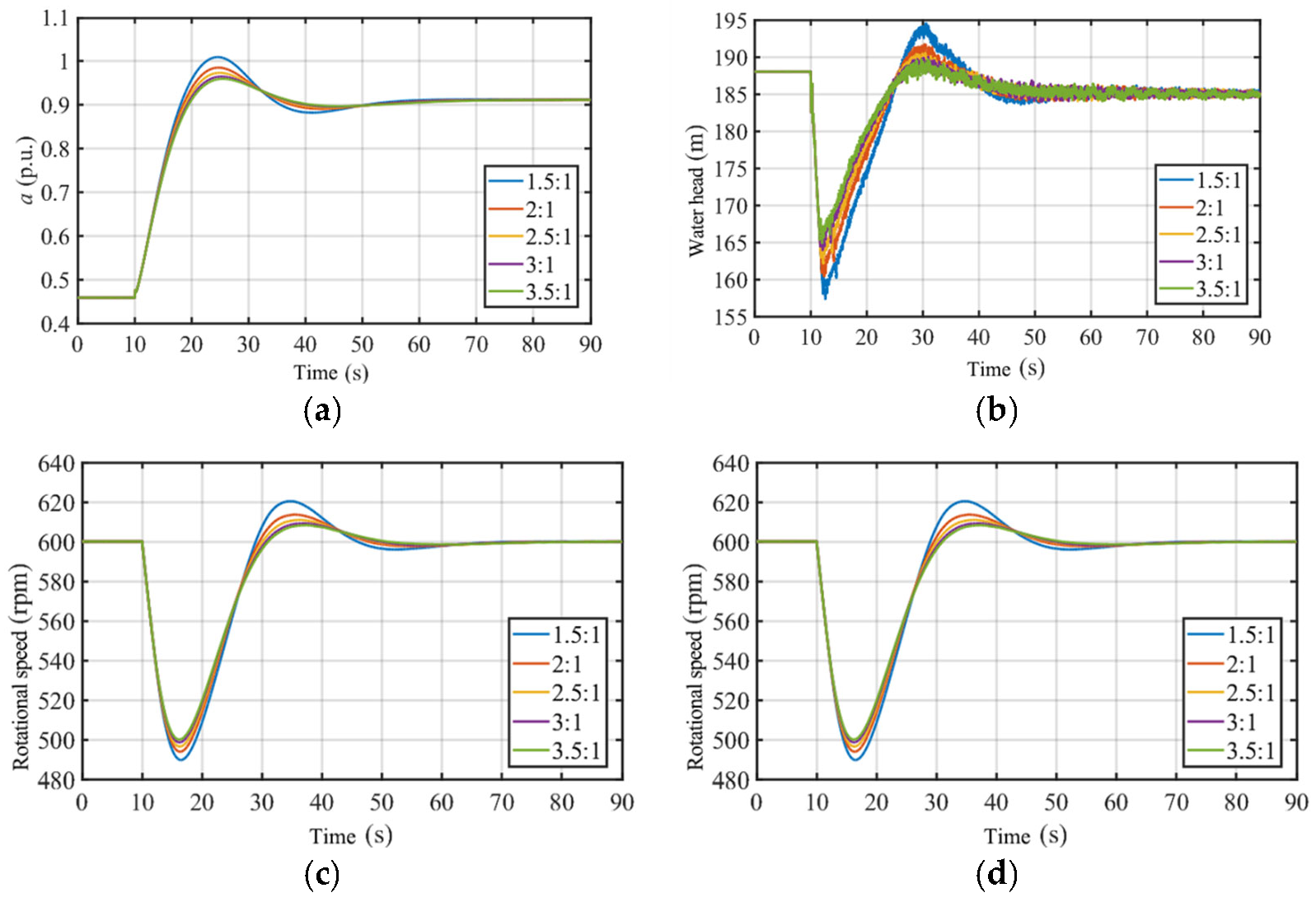
3.1.1. Main Branch Pipe Diameter Ratio

The selection of the pressure diversion pipe diameter is closely related to the investment cost of the hydropower station. A larger diameter pipe requires a higher initial investment; however, if the diameter is too small, it increases the water hammer pressure at the end of the volute, negatively affecting the stable operation of the unit. During large fluctuations in the transition process, the sudden change in water hammer pressure has a greater impact on the unit. Therefore, selecting a reasonable pressure piping main branch pipe diameter ratio is crucial for both the piping design and the safe, reliable operation of the hydropower station. In this paper, the unit load is increased from 50% to the rated load, with the main branch pipe diameter ratio set at 1.3:1, 1.5:1, 1.7:1, 1.9:1, and 2.1:1, respectively. The effect of different pipe diameter ratios on the system stability of the unit during the transition process is investigated. The dynamic response of the unit under these different pipe diameter ratios is shown in Figure 6.

As shown in Figure 6a, the governor automatically tracks the load change and adjusts the active guide vane to ensure that the unit’s rotational speed returns to the vicinity of the rated rotational speed during the load-increasing transition process. Overall, the variation amplitude of the guide vane opening shows an inverse relationship with the main branch pipe diameter ratio. As the diameter ratio decreases, the curve rising rate, peak value, and overshoot all increase. For instance, under diameter ratios from 1.7:1 to 2.1:1, the guide vane openings stabilize around 0.95 p.u., while under the 1.3:1 diameter ratio condition, it reaches 1.03 p.u., maintaining approximately 0.02 p.u. higher after stabilization. In Figure 6b, as the main branch pipe diameter ratio of the hydropower generation system decreases, the unit water head decreases further, and the time required to reach stabilization increases. When the diameter ratio decreases to 1.3:1, the maximum drop in unit water head occurs, with a decrease of 14.98% compared to the rated water head. The variation patterns of unit rotational speed and power with different main branch diameter ratios are shown in Figure 6c,d, respectively. Notably, the trend of unit rotational speed (Figure 6c) closely resembles that of the unit water head (Figure 6b), while the unit power (Figure 6d) follows a similar pattern to the guide vane opening (Figure 6a).

Table 1. Regulation performance index under different main branch pipe diameter ratios.

Pipe Diameter Ratio	Rotational Speed Regultion Time	Rotational Speed Overshoot	Rotational Speed Rise Time	Rotational Speed Peak Time	Inversion Power Peak	Inversion Power Peak Time
1.3:1	34.78	0.180	14.03	26.67	6.00	19.51
1.5:1	33.56	0.170	15.02	27.60	5.67	18.47
1.7:1	31.77	0.163	16.09	28.57	5.53	18.37
1.9:1	20.92	0.159	17.02	29.93	5.46	17.44
2.1:1	21.35	0.156	17.33	30.16	5.41	18.26

presents the regulating performance indicators for different main diameter ratios of the main penstocks. The table shows that when the diameter ratio is 1.3:1, the unit experiences the greatest rotational speed and power fluctuations, with a rotational speed regulation time of 34.78 s, a rotational speed overshoot of 0.180, a rotational speed rise time of 14.3 s, a rotational speed peak time of 26.67 s, an inversion power peak of 6.00 MW, and an inversion power peak time of 19.51 s. Notably, the rotational speed regulation time is most significantly affected by changes in the main branch pipe diameter ratio. The maximum rotational speed regulation time (at 1.3:1 diameter ratio) differs from the minimum (at 1.9:1 diameter ratio) by 13.86 s, representing a year-on-year increase of 66.25%. As a result, the smaller the main branch pipe diameter ratio of the diversion pipeline during the unit’s load-increase transition process, the greater the fluctuations in water head, rotational speed, and power, leading to worse stability in the transition process.

3.1.2. Surge Tank Location

The location of the surge tank takes into account factors such as the role of the unit in the power system, topography, layout of the diversion system, and economic considerations. Therefore, it is necessary to analyze the results of unit system regulation, protection calculations, and operating conditions during the design process, while synthesizing the influence of various factors to select the optimal location for the surge tank. The pipeline length ratios before and after the surge tank are 1.5:1, 2:1, 2.5:1, 3:1, and 3.5:1, respectively, to investigate the effect of different surge tank positions on the stability of the unit during the load-increase transition process. The guide vane opening, unit water head, unit rotational speed, and unit power at different surge tank positions are shown in Figure 7.

As shown in Figure 7a,b, when the load command is issued, the movable guide vanes open quickly, and the unit water head decreases sharply. When the pipeline length ratio before and after the surge tank is 1.5:1, the change in the guide vane opening is the most dramatic, as is the decrease in water head, which is 16.31% lower than the rated water head. Combined with Figure 7c,d and

Table 2. Regulation performance index under different surge tank locations.

Location of the Surge Tank	Rotational Speed Regulation Time	Rotational Speed Overshoot	Rotational Speed Rise Time	Rotational Speed Peak Time	Inversion Power Peak	Inversion Power Peak Time
1.5:1	32.54	0.184	12.64	24.92	6.25	18.31
2.0:1	32.61	0.177	13.35	25.48	5.94	17.58
2.5:1	32.40	0.173	14.03	36.18	5.80	16.59
3.0:1	32.20	0.169	14.57	36.80	5.71	16.79
3.5:1	31.70	0.167	15.00	37.42	5.65	17.34

, it can be seen that the maximum fluctuations in unit rotational speed and power occur when the pipeline length ratio before and after the surge tank is 1.5:1, with a rotational speed regulation time of 32.54 s, a rotational speed overshoot of 0.184, a rotational speed rise time of 12.64 s, a rotational speed peak time of 24.92 s, an inversion power peak of 6.25 MW, and an inversion power peak time of 18.31 s. Moreover, the rotational speed peak time exhibits the most pronounced sensitivity to variations in the pipeline length ratio. The maximum rotational speed peak time (at 3.5:1 pipeline length ratio) differs from the minimum (at 1.5:1 pipeline length ratio) by 12.5 s, corresponding to a significant year-on-year increase of 50.16%. Therefore, the closer the surge tank is to the upstream reservoir, the greater the fluctuations in the unit’s water head, rotational speed, and power, and the worse the unit’s stability.

3.2. The Impact of Operating Conditions on the Stability of the Unit Operation

3.2.1. Initial Load

Hydropower units operate less efficiently when deviating from their rated conditions to accommodate the regulation of intermittent energy fluctuations. The degree of instability is different for different operating conditions. Therefore, 50% rated load, 60% rated load, 70% rated load, 80% rated load, and 90% rated load are taken to investigate the effect of different initial loads on the system stability of the unit during the load increase transition. Figure 8 displays the unit’s dynamic response.

As shown in Figure 8a, the governor opens the movable guide vane to the target opening based on different load changes. The greater the load difference, the steeper the curve, and the larger the rotational speed overshoot. The unit water head drops more and takes longer to stabilize if the initial load is smaller, as shown in Figure 8b. The largest water head drop occurs at 50% load, when the water head drops 8.5% below the rated water head. When combined with

Table 3. Regulation performance index under different initial loads.

Initial Load	Rotational Speed Regulation Time	Rotational Speed Overshoot	Rotational Speed Rise Time	Rotational Speed Peak Time	Inversion Power Peak	Inversion Power Peak Time
50%	21.35	0.152	18.17	30.04	5.38	17.84
60%	20.88	0.115	17.97	30.94	4.06	17.45
70%	20.53	0.081	19.05	31.84	2.77	17.38
80%	19.07	0.050	19.20	31.56	1.71	17.79
90%	14.06	0.018	19.79	30.71	0.63	14.64

and Figure 8c,d, it is evident that the unit’s power and rotational speed fluctuate most when the initial load is 50% of the rated load. This is especially true when the load is suddenly increased. At this point, the rotational speed regulation time is 21.35 s, the rotational speed overshoot is 0.152 s, the rotational speed rise time is 18.17 s, the rotational speed peak time is 30.04 s, the inversion power peak is 5.38 MW, and the inversion power peak time is 17.84 s. Notably, both rotational speed overshoot and inversion power peak show the highest sensitivity to initial load levels. The maximum values of these parameters occur at 50% initial load, while the minimum values appear at 90% load, with approximately an 11-fold difference between the maximum and minimum values. Overall, the lower the initial load during the load increase, the greater the fluctuations in the unit water head, rotational speed, and power, and the less stable the transition process.

3.2.2. Characteristic Water Head

Variations in upstream water inflow and the impact of low water periods cause the unit water head to fluctuate to varying degrees. When the unit system operates at different characteristic water heads, the opening of the movable guide vane varies. In this paper, the unit’s characteristic water heads are taken as the rated water head of 188 m, the maximum water head of 214.52 m, and three intermediate water heads of 196.84 m, 205.68 m, and 223.36 m to investigate the impact of different characteristic water heads on the stability of the system. Figure 9 shows the unit’s dynamic response under different water heads.

As shown in Figure 9a, the smaller the unit water head, the greater the opening of the guide vane at the rated load, resulting in the guide vane moving for a longer duration.

Table 4. Regulation performance index under different water head.

Characteristic Water Head	Rotational Speed Regulation Time	Rotational Speed Overshoot	Rotational Speed Rise Time	Rotational Speed Peak Time	Inversion Power Peak	Inversion Power Peak Time
223.36	16.45	0.125	13.54	23.22	5.55	12.79
214.52	17.30	0.131	14.25	24.64	5.53	13.41
205.68	18.39	0.138	15.37	26.63	5.47	15.02
196.84	19.63	0.144	16.49	28.67	5.42	16.52
188.00	21.35	0.152	18.17	30.04	5.38	17.84

lists the regulatory performance indicators for various characteristic water heads. According to Figure 9c,d and Table 4, when the unit water head is 188 m, the unit rotational speed and power fluctuate the most. At this point, the rotational speed regulation time is 16.45 s, the rotational speed overshoot is 0.125, the rotational speed rise time is 13.54 s, the rotational speed peak time is 23.22 s, the inversion power peak is 5.55 MW, and the inversion power peak time is 12.79 s. Notably, all regulatory performance metrics exhibit relatively small variation gradients under different characteristic water head conditions. No significant differences comparable to those induced by initial load parameters, pipeline configurations, or control parameters are observed. Specifically, the deviations between the maximum and minimum values of these metrics remain limited, with neither extreme oscillations nor statistically discernible anomalies manifesting in the dataset. As a result, the smaller the characteristic water head during the unit’s load increase, the greater the fluctuations in the unit rotational speed and power, and the less stable the unit is at low water heads.

3.3. Influence of Control Parameters on the Stability of Unit Operation

3.3.1. Proportional Gain

When the unit operates in single-unit load-bearing mode, the governing system tracks load changes using frequency control to ensure that the frequency remains close to the rated frequency. The function of the proportional gain is to reflect frequency deviation proportionally; when the load increases, proportional regulation activates to accelerate the regulation and reduce the error. The selection of parameters impacts the system’s stability. As a result, the proportional gain is set to 0.6, 0.8, 1.0, 1.2, and 1.4 to investigate the effect of different proportional gains on the unit’s stability as the load increases. The dynamic response is depicted in Figure 10.

Figure 10a shows that when the proportional gain is 1.4, the guide vane opens relatively quickly, reducing the time required to reach stability. As shown in Figure 10b, as the proportional gain decreases, the greater the unit water head drop, and the longer it takes to reach stabilization. When the proportional gain is 1.4, the maximum drop in unit water head occurs, with a decrease of 10.21% compared to the rated water head. Figure 10c,d depicts and analyzes the performance indicators of primary frequency modulation, as shown in

Table 5. Regulation performance index under different proportional gains.

Proportional Gain	Rotational Speed Regulation Time	Rotational Speed Overshoot	Rotational Speed Rise Time	Rotational Speed Peak Time	Inversion Power Peak	Inversion Power Peak Time
0.6	38.19	0.170	14.81	28.37	5.72	20.25
0.8	34.51	0.160	16.24	28.85	5.53	18.21
1.0	21.35	0.152	18.17	30.04	5.38	17.84
1.2	22.51	0.145	22.46	33.78	5.23	16.69
1.4	24.50	0.138	36.09	36.09	5.12	15.08

. When the proportional gain is 0.6, the unit rotational speed and power fluctuations peak, with a rotational speed regulation time of 38.19 s, a rotational speed overshoot of 0.170, a rotational speed rise time of 14.81 s, a rotational speed peak time of 28.37 s, an inversion power peak of 5.72 MW, and an inversion power peak time of 20.25 s. Notably, the rotational speed regulation time demonstrates the highest sensitivity to variations in proportional gain. The maximum rotational speed regulation time (at proportional gain 0.6) differs from the minimum (at proportional gain 1.4) by 16.84 s, corresponding to a staggering year-on-year increase of 143.69%. Therefore, the smaller the proportional gain, the greater the fluctuations in the unit water head, rotational speed, and power, and the lower the stability during the transition process.

3.3.2. Integral Gain

Compared to proportional gain, integral gain maintains the unit’s frequency near the rated frequency and helps eliminate residual differences. The integral gain of the unit’s governing system is set to 0.6, 0.8, 1.0, 1.2, and 1.4 to investigate the impact of different integral gains on the stability of the unit. The dynamic response is shown in Figure 11.

Figure 11a shows that when the integral gain is 0.29, the guide vane responds quickly, but the overshoot is large, and the time to reach stability is longer. Figure 11b shows that as the integral gain increases, the drop in the unit water head becomes greater, and the time required to reach stability increases. The maximum drop in the unit water head occurs at 0.29, with an 8.83% decrease compared to the rated water head. Figure 11c,d and

Table 6. Regulation performance index under different integral gains.

Integral Gain	Rotational Speed Regulation Time	Rotational Speed Overshoot	Rotational Speed Rise Time	Rotational Speed Peak Time	Inversion Power Peak	Inversion Power Peak Time
0.21	25.45	0.155	26.27	37.79	5.19	19.26
0.23	23.17	0.153	21.31	33.00	5.25	17.41
0.25	21.35	0.152	18.17	30.04	5.38	17.84
0.27	20.01	0.151	16.28	27.67	5.46	17.14
0.29	18.87	0.149	14.77	26.65	5.57	16.36

show that when the integral gain is 0.29, the fluctuation in unit rotational speed and power is maximal, with a rotational speed regulation time of 18.87 s, a rotational speed overshoot of 0.149, a rotational speed rise time of 14.77 s, a rotational speed peak time of 26.65 s, an inversion power peak of 5.57 MW, and an inversion power peak time of 16.36 s. Notably, the most sensitive performance parameter to integral gain variations aligns with the effect of proportional gain—the rotational speed rise time. However, contrary to previous observations, the maximum rotational speed rise time (26.27 s) occurs at the minimum integral gain (0.21), whereas the minimum value (14.77 s) appears at the maximum integral gain (0.29), resulting in an absolute difference of 11.5 s and a year-on-year increase of 77.86%. To summarize, as the load on the unit system increases, the higher the integral gain, the greater the variation in the unit water head, rotational speed, and power, and the worse the unit’s stability.

3.4. Sensitivity Analysis of Unit Dynamic Response

The previous section examined the impact of structural design parameters, operating conditions, and system control parameters on the unit’s operating characteristics during load increases. Based on the results, the initial input parameters were selected within a ±10% range of values. The effect of each 1% variation in input parameters on operating characteristics was measured. The sensitivity of each parameter to various performance indicators was examined, and the influence of different structural-operating-control input parameters on the unit system’s operating characteristics was compared. This analysis serves as a reference for structural design and the safe and stable operation of hydropower systems. Figure 12, Figure 13, Figure 14, Figure 15, Figure 16 and Figure 17 depict sensitivity heat maps and radar charts for the rotational speed regulation time, rotational speed overshoot, rotational speed rise time, rotational speed peak time, inversion power peak, and inversion power peak time for various structural operating control input parameters.

The sensitivity of the unit’s regulation performance indicators to various structural-operational-control characteristics varies significantly, as shown in Figure 12, Figure 13, Figure 14, Figure 15, Figure 16 and Figure 17. Among them, the proportional gain is the most sensitive to the rotational speed regulation time, while the pipe diameter ratio is the least sensitive. The sensitivity ranking of each structural-operational-control parameter to the radar chart’s rotational speed regulation time is as follows: proportional gain > surge tank location > initial load > integral gain > characteristic water head > pipe diameter ratio. In terms of rotational speed overshoot, the initial load has the highest sensitivity, while the other parameters have relatively low sensitivity, with the following ranking: initial load > surge tank location > pipe diameter ratio > integral gain > characteristic water head > proportional gain. The integral gain has the greatest impact on the rotational speed rise time, followed by the characteristic water head, in this order: integral gain > characteristic water head > surge tank location > proportional gain > pipe diameter ratio > initial load. The characteristic water head has the greatest influence on rotational speed peak time, followed by integral gain, surge tank location, proportional gain, pipe diameter ratio, and initial load. The initial load is the most sensitive to the inversion power peak, with the following sensitivity ranking: initial load > surge tank location > integral gain > characteristic water head > proportional gain > pipe diameter ratio. The characteristic water head is the most sensitive to the inversion power peak time, with the following order: characteristic water head > pipe diameter ratio > initial load > integral gain > surge tank location > proportional gain.

4. Discussion

This study delved into the influence of structural, operational, and control parameters on the stability of hydropower units during the load-increasing transition process by constructing a coupled hydraulic–mechanical–electrical model and conducting parameter sensitivity analysis. The research findings not only lay a theoretical foundation for the optimal selection of hydropower unit parameters but also reveal numerous issues worthy of in-depth exploration and future research directions.

On the one hand, with the large-scale integration of renewable energy, the power system is evolving towards a multi-energy complementary direction. Future research can couple hydropower units with other energy forms, such as wind, solar, and energy storage, to explore their interaction and coordinated operation mechanisms. For example, stochastic differential equations can be introduced to describe the power fluctuations of intermittent renewable energy, and a generalized sensitivity index system for the multi-energy coupling of water–wind–solar–storage can be established to improve the stability theory of the new-type power system dominated by renewable energy.

On the other hand, this study may have overlooked uncertain factors such as equipment aging and environmental factor changes during the modeling process. In the future, uncertainty analysis methods can be introduced to consider the impact of these factors on unit stability, thereby enhancing the robustness and reliability of the model. For instance, methods like Monte Carlo simulation can be used to quantitatively analyze the uncertainty of parameters, providing a more reliable decision-making basis for the design and operation of hydropower stations.

5. Conclusions

In the design and operation of hydropower plants, unsuitable parameters can affect the plant’s stability. This paper uses a hydropower station model to investigate the impact of various structural design characteristics, operating condition parameters, and control parameters on the stability of the system during load increases. The main conclusions are as follows:

• Increasing the main branch pipe diameter ratio and the distance between the surge tank and the upstream reservoir improves stability during the transition. Among these factors, the main branch pipe diameter ratio is most sensitive to the inversion power peak time, while the surge tank’s position shows strong sensitivity to the rotational speed regulation time.
• A larger initial load and characteristic water head enhance the stability of the hydropower plant during the load increase transition process. Among these, the initial load shows strong sensitivity to rotational speed overshoot and inversion power peak, while the characteristic water head is highly sensitive to the rotational speed rise time, rotational speed peak time, and inversion power peak time.
• Lowering the proportional gain and increasing the integral gain reduces the stability of the hydropower plant system during the transition process. The sensitivity analysis shows that the proportional gain (K_p) is highly sensitive to the rotational speed regulation time, while the integral gain (K_i) strongly affects the rotational speed rise time.

References

1. Bao, H.Y.; Long, L.T.; Fu, L.; Wei, J.F. Study on stability of load regulation transition process of hydro turbine governor in power mode. Trans. Chin. Soc. Agric. Eng. 2019, 35, 50–57, (In Chinese with English abstract). [Google Scholar] [CrossRef]
2. Binama, M.; Su, W.-T.; Li, X.-B.; Li, F.-C.; Wei, X.-Z.; An, S. Investigation on pump as turbine (PAT) technical aspects for micro hydropower schemes: A state-of-the-art review. Renew. Sustain. Energy Rev. 2017, 79, 148–179. [Google Scholar] [CrossRef]
3. Zhang, B.T. Energy Revolution Inevitable, Pumped Storage Thriving. Hydropower Pumped Storage 2017, 3, 5. Available online: http://old.hydropower.org.cn/showNewsDetail.asp?nsId=22105 (accessed on 13 October 2024). (In Chinese with English abstract).
4. Yang, W.; Norrlund, P.; Chung, C.Y.; Yang, J.D.; Lundin, U. Eigen-analysis of hydraulic-mechanical-electrical coupling mechanism for small signal stability of hydropower plant. Renew. Energy 2018, 115, 1014–1025. [Google Scholar] [CrossRef]
5. Khalid, M.; AlMuhaini, M.; Aguilera, R.P.; Savkin, A.V. Method for planning a wind–solar–battery hybrid power plant with optimal generation-demand matching. IET Renew. Power Gen. 2018, 12, 1800–1806. [Google Scholar] [CrossRef]
6. Zhang, H.; Hu, P. Study on regulating oscillation in multi hydro turbine generators sharing flow channel structure of tailrace surge tank. J. Hydraul. Eng. 2015, 46, 10. Available online: http://jhe.ches.org.cn/jhe/ch/reader/view_abstract.aspx?file_no=201502013 (accessed on 1 December 2024). (In Chinese with English abstract).
7. Goyal, R.; Gandhi, B.K. Review of Hydrodynamics Instabilities in Francis Turbine During Off-design and Transient Operations. Renew. Energy 2018, 116, 697–709. [Google Scholar] [CrossRef]
8. Li, H.H.; Xu, B.B.; Arzaghi, E.; Abbassi, R.; Chen, D.Y.; Aggidis, G.A.; Zhang, J.J.; Patelli, E. Transient Safety Assessment and Risk Mitigation of a Hydroelectric Generation System. Energy 2020, 196, 117135. [Google Scholar] [CrossRef]
9. Liu, Y.N.; Yang, J.D.; Zeng, W. Setting conditions of surge chambers at hydropower station in elastic model based on operation stability. J. Hydroelectr. Eng. 2016, 35, 6, (In Chinese with English abstract). [Google Scholar] [CrossRef]
10. Kamal, M.M.; Abbas, A.; Prasad, V.; Kumar, R. A numerical study on the performance characteristics of low head Francis turbine with different turbulence models. Mater. Today Proc. 2022, 49, 349–353. [Google Scholar] [CrossRef]
11. El-Sapa, S.; Lotfy, K.; El-Bary, A. Impact of laser short-pulse heating and variable thermal conductivity on photo-elasto-thermodiffusion waves of fractional heat excited semiconductor. J. Electromagn. Waves Appl. 2022, 36, 2628–2646. [Google Scholar] [CrossRef]
12. El-Sapa, S.; Lotfy, K.; El-Bary, A.A. Non-local semiconductor photothermal excitation medium in moisture diffusivity subjected to heating by pulsed laser. Eur. Phys. J. Plus 2023, 138, 368. [Google Scholar] [CrossRef]
13. El-Sapa, S.; Lotfy, K.; El-Bary, A. Laser short-pulse impact on magneto-photo-thermo-diffusion waves in excited semiconductor medium with fractional heat equation. Acta Mech. 2022, 233, 3893–3907. [Google Scholar] [CrossRef]
14. Celebioglu, K.; Altintas, B.; Aradag, S.; Tascioglu, Y. Numerical research of cavitation on Francis turbine runners. Int. J. Hydrogen Energy 2017, 42, 17771–17781. [Google Scholar] [CrossRef]
15. Yang, W.; Norrlund, P.; Saarinen, L.; Yang, J.; Guo, W.; Zeng, W. Wear and tear on hydro power turbines—Influence from primary frequency control. Renew. Energy 2016, 87, 88–95. [Google Scholar] [CrossRef]
16. Valentín, D.; Presas, A.; Egusquiza, E.; Valero, C.; Egusquiza, M.; Bossio, M. Power Swing Generated in Francis Turbines by Part Load and Overload Instabilities. Energies 2017, 10, 2124. [Google Scholar] [CrossRef]
17. Zhang, L.; Wu, Q.Q.; Ma, Z.Y.; Wang, X.N. Transient vibration analysis of unit-plant structure for hydropower station in sudden load increasing process. Mech. Syst. Signal Process. 2019, 120, 486–504. [Google Scholar] [CrossRef]
18. Ma, W.C.; Zhao, Z.G.; Yang, J.B.; Lai, X.; Liu, C.P.; Yang, J.D. A transient analysis framework for hydropower generating systems under parameter uncertainty by integrating physics-based and data-driven models. Energy 2024, 297, 131141. [Google Scholar] [CrossRef]
19. Zhu, Z.; Tan, X.; Lu, X.; Liu, D.; Li, C. Hopf bifurcation and parameter sensitivity analysis of a doubly-fed variable-speed pumped storage unit. Energies 2022, 15, 204. [Google Scholar] [CrossRef]
20. Lei, L.W.; Li, F.; Kheav, K.L.; Jiang, W.; Luo, X.Q.; Patelli, E.; Xu, B.B.; Chen, D.Y. A start-up optimization strategy of a hydroelectric generating system: From a symmetrical structure to asymmetric structure on diversion pipes. Renew. Energy 2021, 180, 1148–1165. [Google Scholar] [CrossRef]
21. Li, W.X. Study on the Hydraulic Transition Process Calculation of Three Different Arrangements of Tailwater Pressure Chamber. Master’s Thesis, Xi’an University of Technology, Xi’an, China, 2021. (In Chinese with English abstract). [Google Scholar]
22. Liao, Y.W.; Yang, W.J.; Zhao, Z.G.; Li, X.D.; Ci, X.H.; Bidgoli, M.A.; Yang, J.D. Influence mechanism of backlash nonlinearity on dynamic regulation stability of hydropower units. Sustain. Energy Technol. Assess. 2022, 51, 101917. [Google Scholar] [CrossRef]
23. Liu, H.; Fan, B.Y.; Tang, C.; Ge, S.Y.; Wang, Y.; Guo, L. Game theory based alternate optimization between expansion planning of active distribution system and siting and sizing of photovoltaic and energy storage. Autom. Electr. Power Syst. 2017, 41, 38–45, 116. Available online: https://epjournal.csee.org.cn/dlxtzdh/article/id/564fb3c1-4b09-489c-a3ae-210fd7d344a5 (accessed on 4 December 2024). (In Chinese with English abstract).
24. Singh, M.K.; Naresh, R.; Gupta, D.K. Optimal tuning of temporary droop governor of hydro power plant using genetic algorithm. In Proceedings of the 2013 International Conference on Energy Efficient Technologies for Sustainability, Nagercoil, India, 10–12 April 2013; pp. 1132–1137. [Google Scholar] [CrossRef]
25. Feng, X.Y. Analysis of the Transient Performance of the Water Turbine Regulation System. Master’s Thesis, North China University of Water Resources and Electric Power, Baoding, China, 2016. (In Chinese with English abstract). [Google Scholar]
26. Riasi, A.; Tazraei, P. Numerical analysis of the hydraulic transient response in the presence of surge tanks and relief valves. Renew. Energy 2017, 107, 138–146. [Google Scholar] [CrossRef]
27. Guo, W.C.; Peng, Z.Y. Hydropower system operation stability considering the coupling effect of water potential energy in surge tank and power grid. Renew. Energy 2019, 134, 846–861. [Google Scholar] [CrossRef]
28. Hou, J.J.; Li, C.S.; Guo, W.C.; Fu, W.L. Optimal successive start-up strategy of two hydraulic coupling pumped storage units based on multi-objective control. Int. J. Electr. Power Energy Syst. 2019, 111, 398–410. [Google Scholar] [CrossRef]
Figure 1. Schematic diagram of the hydropower generation system.
Energies 18 02609 g001
Figure 2. The schematic diagram of the method of characteristics.
Energies 18 02609 g002
Figure 3. The schematic diagram of boundary conditions for each node of the water diversion system: (a) upstream reservoir; (b) downstream reservoir; (c) surge tank; (d) elbow pipe; (e) bifurcated pipe; (f) hydro-turbine.
Energies 18 02609 g003
Figure 4. The characteristic curves of hydro-turbine. (a) Flow characteristic curve; (b) torque characteristic curve.
Energies 18 02609 g004
Figure 5. PID governor input–output response block diagram.
Energies 18 02609 g005
Figure 6. Dynamic response of the unit under different pipe diameter ratios. (a) Guide vane opening; (b) unit water head; (c) unit rotational speed; (d) unit power.
Energies 18 02609 g006
Figure 7. Dynamic response of the unit under different surge tank locations. (a) Guide vane opening; (b) unit water head; (c) unit rotational speed; (d) unit power.
Energies 18 02609 g007
Figure 8. Dynamic response of the unit under different initial loads. (a) Guide vane opening; (b) unit water head; (c) unit rotational speed; (d) unit power.
Energies 18 02609 g008
Figure 9. Dynamic response of the unit under different water heads. (a) Guide vane opening; (b) unit water head; (c) unit rotational speed; (d) unit power.
Energies 18 02609 g009
Figure 10. Dynamic response of the unit under different proportional gains. (a) Guide vane opening; (b) unit water head; (c) unit rotational speed; (d) unit power.
Energies 18 02609 g010
Figure 11. Dynamic response of the unit under different integral gains. (a) Guide vane opening; (b) unit water head; (c) unit rotational speed; (d) unit power.
Energies 18 02609 g011
Figure 12. Sensitivity of different input parameters to the rotational speed regulation time. (a) Sensitivity heat map; (b) radar map.
Energies 18 02609 g012
Figure 13. Sensitivity of different input parameters to the rotational speed overshoot. (a) Sensitivity heat map; (b) radar map.
Energies 18 02609 g013
Figure 14. Sensitivity of different input parameters to the rotational speed rise time. (a) Sensitivity heat map; (b) radar map.
Energies 18 02609 g014
Figure 15. Sensitivity of different input parameters to the rotational speed peak time. (a) Sensitivity heat map; (b) radar map.
Energies 18 02609 g015
Figure 16. Sensitivity of different input parameters to the inversion power peak. (a) Sensitivity heat map; (b) radar map.
Energies 18 02609 g016
Figure 17. Sensitivity of different input parameters to the inversion power peak time. (a) Sensitivity heat map; (b) radar map.
Energies 18 02609 g017