Machine Learning-Based Forecasting of Temperature and Solar Irradiance for Photovoltaic Systems

Abstract

The integration of photovoltaic (PV) systems into the global energy landscape has been boosted in recent years, driven by environmental concerns and research into renewable energy sources. The accurate prediction of temperature and solar irradiance is essential for optimizing the performance and grid integration of PV systems. Machine learning (ML) has become an effective tool for improving the accuracy of these predictions. This comprehensive review explores the pioneer techniques and methodologies employed in the field of ML-based forecasting of temperature and solar irradiance for PV systems. This article presents a comparative study between various algorithms and techniques commonly used for temperature and solar radiation forecasting. These include regression models such as decision trees, random forest, XGBoost, and support vector machines (SVM). The beginning of this article highlights the importance of accurate weather forecasts for the operation of PV systems and the challenges associated with traditional meteorological models. Next, fundamental concepts of machine learning are explored, highlighting the benefits of improved accuracy in estimating the PV power generation for grid integration.

1. Introduction

The proliferation of photovoltaic (PV) has brought about significant changes in the global energy landscape. With the sun as an abundant and renewable energy resource, PV installations have become a vital component of efforts to reduce greenhouse gas emissions and transition towards a greener future. However, the proficiency and functioning of PV systems are inherently linked to the availability of sunlight, which is subject to dynamic fluctuations driven by meteorological factors such as temperature and solar irradiance. Solar energy is produced using PV cells, which transform sunlight to produce electricity. The efficacy and staging of solar power systems are strongly influenced by solar irradiance, which is the amount of sunlight received on a specified surface during a specific period. Due to the growing use of electricity from solar energy on the one hand and the growth of this energy integration into the electricity grid on the other hand [1,2], it is becoming increasingly important to predict the amount of this renewable energy source. This prediction must imperatively involve the forecasting of meteorological data such as irradiation and temperature. In this context, as mentioned by Yagli et al. [3], an improvement in the accuracy of photovoltaic energy production forecasting by 25% could reduce 1.56% (USD 46.5 million) in net production costs. Consequently, weather and photovoltaic power forecasting is essential to assess solar potential.

Numerous photovoltaic power-forecasting approaches have been studied. According to Mellit et al. [4] and taking into account the horizon [5], these approaches can be classified into four categories: (1) very short-term forecasting (VSTF), (2) short-term forecasting (STF), (3) medium-term (MTF), and (4) long-term forecasting (LTM). According to the same authors [4], each category has its precise application; for example, very short-term forecasting is used in the management of microgrids. Accurate prediction of temperature and solar irradiance is essential for the optimization of a grid-connected PV system operation. Numerous works have been done to recommend an accurate solar energy prediction. The authors in [6,7] discussed two main approaches: traditional (conventional) approaches and AI (artificial intelligence) approaches. Traditional approaches contain physical methods, statistical methods, and regression methods used for energy prediction [8]. These methods served as a cornerstone for weather forecasting. They can deliver good accuracy, but they mostly depend on the stability of weather conditions. However, the implementation of conventional models is comparatively difficult and requires different parameters and expensive equipment.

On the other hand, over the past decades, AI methods have become very popular in different engineering fields [6]. Among AI algorithms, machine learning (ML) has become a powerful tool, offering the potential to advance the accuracy and reliability of forecasts. The forecasting horizon, spatial resolution, and the accessibility of historical data are just some of the variables that affect the accuracy of temperature and solar irradiance forecasts [4]. Smaller spatial areas and shorter forecast lead times often result in more accurate forecasts. When you have a wealth of reliable historical data, forecasts are also more accurate. The principle of ML relies on models learned from large data sets and uses these models to forecast unknown data by learning from mistakes and comparing errors [9]. Machine learning frequently deals with classification and regression problems using different algorithms and techniques such as random forest, XGBoost, support vector machine, and the decision tree.

This article presents an in-depth analysis of existing machine-learning models used in temperature and solar irradiance prediction. The present work shows how ML models can be trained on historical data to learn the relationships between temperature, irradiance, and other relevant factors, such as month, season, and weather conditions. Once trained, these models can be used to predict future temperature and irradiance values accurately. This study evaluates the effectiveness and accuracy of presented ML models for weather forecasting. Moreover, given the self-adaptive nature of ML models, this study and the application of these models to weather forecasts for PV systems remain sustainable since they are based on models that are capable of evolution [10].

The rest of this paper is organized as follows: Section 2 presents the motivation of the present study; related works are presented in Section 3; Section 4 brings together the ML algorithms employed to predict solar irradiance and temperature proposed and studied in this work. In Section 5, the results found are discussed. Section 6 presents some conclusions.

2. Motivation of This Study

Electricity production and consumption must always be precisely balanced by an electric operator. The ability of the electricity system to absorb anticipated and unanticipated changes and interruptions (in production and consumption) while maintaining quality and consistency of service to customers is then what determines the reliability of the electricity system. The energy supplier will then be responsible for monitoring the system during different periods. The intermittent nature of sustainable energy sources makes it more difficult to manage the network and maintain the production/consumption balance when added to a network [11], which can cause certain problems regarding the security of the network [12]. In addition to voltage fluctuations, poor local power quality, and stability issues, solar power generation is sporadic and unpredictable, leading to several other problems. For example, maintenance operations are necessary on the network because various power plants should be frequently stopped or restarted to ensure the balance between energy production and energy consumption [13]. As a result, the failure rate will increase, and maintenance will require more components [14]. All of these problems increase the cost of photovoltaic energy [15] and greenhouse gas emissions [16].

For this reason, it is essential to develop accurate electricity production projections to strengthen the stability of the integration of a solar PV system’s production into the grid and help producers successfully implement their operational strategies [17]. It is also necessary for reserve estimation, electricity system planning, congestion control, optimal storage management with stochastic production, the exchange of produced energy on the electricity market, and, in the long term, minimizing the cost of electricity production. Several works have been carried out to achieve all these goals, focusing on the accuracy of solar irradiance prediction, which has recently been improved through the use of deep learning and machine learning approaches [18,19].

The choice of decision trees, support vector machines (SVMs), random forest, and XGBoost is based on some good reasons. Decision trees help us understand the decision-making process, making it easier to interpret solar and temperature predictions. These models are great at handling complex, non-linear relationships in weather patterns. SVMs work well with lots of variables, like in meteorological data, ensuring accurate forecasting. They are also robust, meaning they avoid making predictions that are too specific, making them more reliable. Random forest combines multiple decision trees, giving us better predictions and telling us which weather factors matter most. XGBoost improves itself over time, learning from mistakes to refine forecasts. Plus, it handles missing data, which is important in real-world situations where we might not have all the meteorological information. In simple terms, these models are ideal for obtaining accurate temperature and solar energy forecasts for PV systems.

3. Related Work

In the context of photovoltaic systems, there is a renewed interest and creativity in research on temperature and solar irradiation prediction based on machine learning.

Table 1. Bibliographic summary of the main methods and applications.

Ref.	Description	Forecasting Target	Year
[17]	Utilization of a” Partial Functional Linear Regression Model” (PFLRM) for forecasting the daily power generation in photovoltaic (PV) systems in order to capitalize on the substantial trajectory data inherent in daily power output.	PV power	2022
[18]	A comprehensive examination of various resources and techniques employed in predicting solar irradiance across different timeframes.	Solar irradiance	2020
[20]	Determination of a range for ambient temperature and the sun radiant, utilizing MAE as a metric for irradiance, the proportion of variation in these factors.	Temperature and solar	2021
[21]	Various forecasting challenges, comprising eight papers that delve into methods for maximizing the output power of PV systems, the sun radiant, and power generation forecasting.	Solar irradiance, temp., thermal energy production	2022
[22]	Overview of recent studies emphasizing solar irradiance forecasting using ensemble methods categorized into two main forecasting ensembles: competitive and cooperative.	PV power	2023
[23]	A critical and systematic review of current machine learning forecasters for wind and solar power, specifically focusing on (ANNs), (RNNs), (SVMs), and (ELMs).	PV power	2021
[24]	Emerging utilization of alternative methods, including regression trees, random forests, gradient boosting, and various others, in the context of solar irradiation prediction.	Solar irradiance	2017
[25]	Ability to pinpoint seven crucial perspectives and trends for prospective investigations in solar forecasting. These findings are designed to help readers better utilize these approaches for more profound future research.	Solar irradiance, PV power	2023
[26]	Examining the current state of the art and assessing different methodologies, not solely based on their performance and generalization of this. Evaluation of these approaches to perform not only on the designated dataset but also on alternative datasets or varied case studies.	PV power	2018

illustrates some research works related to the present study, and

Table 2. Disadvantages and advantages of ML methods.

Ref.	Machine Learning Method	Advantages	Disadvantages
[17]	Partial functional linear regression model (PFLRM)	Introduces the PFLRM as a generalization of traditional multiple linear regression, allowing the modeling of non-linearity structures in the data.	Acknowledges the need for further investigation and considering additional time-varying meteorological variables as functional predictors.
[18]	RNN, LSTM, GRU, TCN	Leverages deep learning and machine learning techniques for very short-term solar forecasting, demonstrating irradiance and practical application of advanced technologies in renewable energy optimization.	The study’s findings are tailored to the local city of Karachi, potentially limiting the generalizability of the results to other regions with different climatic conditions.
[20]	Machine learning, linear statistical models, numerical weather prediction (NWP)	Guide future research by highlighting the most suitable forecasting methods and confirm the importance of forecasting terms, revealing up to 95% power output variation between short and long-term predictions.	Limitations related to the availability of historical information for site-specific applications potentially impact the model’s accuracy and generalizability.
[21]	Numerical weather prediction models (NWP), physical techniques, machine learning techniques, linear statistical models	Demonstrating a practical strategy for overcoming challenges in inaccurately predicting power generation.	Lack of universally applicable models and the need for customization based on regional characteristics.
[22]	Competitive ensemble (bagging, boosting, ensemble Kalman filter), cooperative ensemble (ARMA-ANN, ARIMA-SVM…)	Demonstrated that ensemble models perform better than standalone ones. The artificial neural network (ANN) and space vector machine (SVM) are widely used with ensemble models (WD-ANN, EMD BPNN, and W-SVM) due to their ability to solve complex.	It did not present the various intelligent techniques and machine learning algorithms used in the field of forecasting, showing the advantages and disadvantages.
[23]	ANN, RNN, SVM, ELM	Compares machine learning methods, metaheuristics, and hybrid approaches, aiding scientists and engineers in choosing suitable prediction methods for diverse circumstances.	Extreme learning machines (ELMs) might be suitable only for simple models and could struggle to capture enough features and learn adequately, requiring careful optimization or extension to become deep networks.
[24]	Regression tree, random forest, gradient boosting	Recognizes the potential of hybrid models and ensemble forecast approaches to enhance prediction performance, addressing the challenges posed by the diversity of solar radiation data.	Due to the variety in data conditions and parameters, determining the superior method becomes challenging, leading to comparable prediction errors among different approaches.
[25]	128 forecasting methods of solar irradiance and power	Reviews five classifications and seven pre-processing methods for solar forecasting data, enhancing forecasting accuracy and providing a solid foundation for further research.	Despite the comprehensive comparisons, the diversity of forecasting methods and associated characteristics makes it challenging to draw definitive conclusions, highlighting the complexity of solar forecasting evaluation.
[26]	Probabilistic forecasting of solar power (PSPF) and load forecasting (PLF)	Recognizes the need to combine PSPF and PLF in the review, emphasizing the growing interest in net demand forecasting and exploring common ground between these areas.	Research gaps such as the impact of net demand forecasting on probabilistic performance metrics and the importance of benchmark datasets.

highlights the advantages/disadvantages of the ML methods used.

When comparing forecasting models based on criteria such as efficiency, complexity, response time, data size, scalability, evaluation methods, difficulty of implementation, and the overall cost of implementation, various considerations come into play (

Table 3. Comparison between ML methods and different “traditional” forecasting methods.

Methods	Accuracy	Complexity Level	Response	Data Size	Scalability	Evaluation	Difficulty of Implementation	Cost
Machine Learning Methods [23,24]	High	high	Slow	Large	Scalable	Statistical metrics (MAE, MSE) and specialized metrics (accuracy, F1-score)	May range from easy to hard	May vary from moderate to high
Statistical Methods [17,19,20]	Good	Simple	Fast	Small	Generally scalable	Statistical metrics (MAE, MSE, RMSE)	Generally easy	Generally low
Physical Methods [9,11]	Good	Varied	Varied	Varied	Moderate	Utilizing physical principles	Can be challenging	Can vary from moderate to high
Numerical Weather Prediction (NWP) Models [12,13]	Good	Varied	slow	Large	Typically scalable	Brier score, continuous ranked probability score	Can be challenging	Generally high
Hybrid Models [25,27]	High	high	Varied	Varied	Moderate	Combine metrics from both statistical and machine learning evaluation	May range from easy to hard	Can vary from moderate to high
Ensemble Forecasting [22]	High	Moderate to high	Varied	Varied	Scalable	Combine metrics from both statistical and machine learning evaluation	May range from easy to hard	Can vary from moderate to high

). Statistical methods, known for their simplicity, demonstrate their efficiency in terms of computational resources and response time, making them suitable for smaller datasets. However, they may have difficulty dealing with complex patterns. Machine learning methods, while potentially offering high accuracy, often require significant computing resources and have slower response times. Physical methods, incorporating fundamental principles, offer moderate efficiency and scalability but may encounter challenges in diverse datasets. Numerical weather prediction (NWP) models, designed for atmospheric forecasting, demonstrate high accuracy but come with high implementation costs and computational requirements. Hybrid models aim to strike a balance between accuracy and efficiency by combining machine learning and physical components. Ensemble methods, focusing on diversity for accuracy, have moderate scalability but may require additional computational resources. Implementation costs vary, with statistical models being cost-effective, machine learning and physical models having moderate to high costs, and hybrid and ensemble models providing a balance between accuracy and implementation expense. The choice of model depends on the specific task requirements, available resources, and acceptable tradeoffs between accuracy, efficiency, and cost.

New irradiation and temperature prediction methods quantify the impact of proposed improvements on the overall efficiency, sustainability, and profitability of photovoltaic systems using more complex models and more precise data. They integrate climate variability, site-specific characteristics, and solar panel performance to provide more reliable forecasts. Compared to traditional forecasting methods, which often rely on simplified models and historical data, new methods provide a better understanding of future weather conditions, enabling more accurate planning and optimized use of photovoltaic systems.

4. Methods

The subfield of machine learning in computer science is classified as an artificial intelligence technique. It has the advantage of allowing models to solve problems that explicit methods cannot, and it can be used in a variety of domains [24]. Analyzing data using machine learning (ML) allows computer systems to gain insights from data over time. Unlike statistical models, ML approaches can generally capture non-linearity and adapt data instability, producing more accurate predictors. As a result, ML algorithms have been used in recent years to forecast a variety of problems, including forecasting renewable energy sources [23].

4.1. Decision Tree

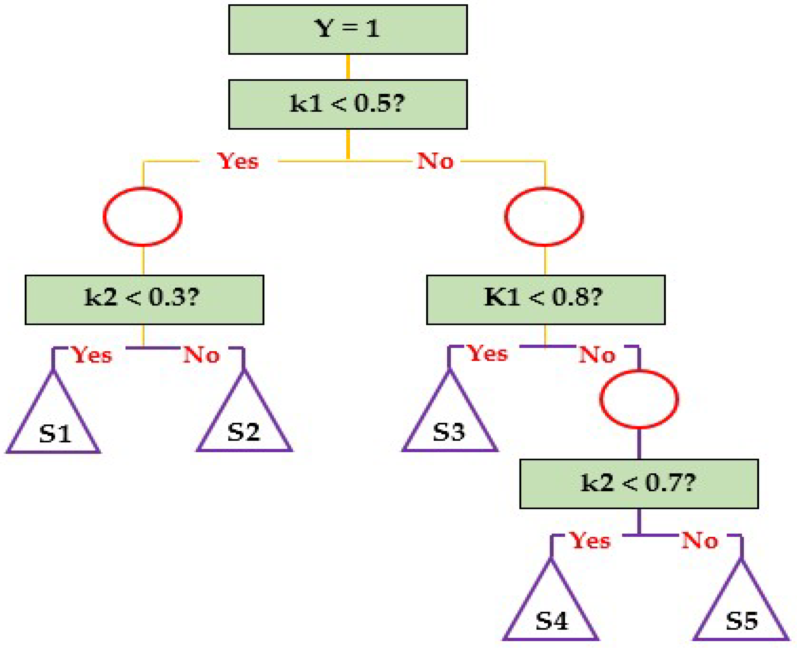
A decision tree (DT) functions as a classification model, illustrating a recursive division of instance space. The structure comprises nodes, forming a rooted tree where the “root” node lacks outgoing edges, and subsequent nodes possess exactly one incoming edge. Internal or test nodes, with exterior edges, partition the instance space based on discrete functions of input attribute values. Each internal node creates two or more subspaces, where, in the simplest scenario, each test assesses a single attribute, dividing the instance space based on attribute values. Numeric attributes are split based on range conditions.

It is common practice to assign a class corresponding to the ideal target value to each leaf. Alternatively, a leaf may store a probability vector indicating the likelihood of the target characteristic having a specific value. Instances are categorized by traversing the tree from the root to a leaf based on test results. The representation employs circles for internal nodes and triangles for leaves [28].

Figure 1 illustrates a straightforward decision tree model with two variables, k1 and k2 (ranging from 0 to 1) and a binary objective variable, Y (0 or 1). A decision tree model has key components, including nodes, branches, and essential modeling operations such as stopping, splitting, and pruning.

• Nodes: Three node types exist. (a) A root node, or decision node, divides records into mutually exclusive sets. (b) Inner nodes, or chance nodes, elucidate options at a particular position in the tree structure, connecting to parent nodes above and child or leaf nodes below. (c) Leaf nodes, or final nodes, signify the result of a sequence of choices or events.
• Branches: Replacing random events from internal and root nodes, branches form a hierarchy, defining decision paths. Each route (from the root node through inner nodes to a leaf node) depicts a rule of classification decision, expressible as ‘if-then’ rules. For instance, “If condition 1 and condition 2 and… condition i occur, then outcome j occurs”.
• Splitting: Parent nodes are divided into purer child nodes related to the target variable, using input variables associated with the target. Continuous and discrete input variables, categorized into two or more bins, are employed. Criteria like entropy, Gini index, classification error, information gain, gain ratio, and towing criteria determine the most crucial input variables, ensuring the purity of resulting child nodes (i.e., the proportion with the target condition) [29].

4.2. Random Forest

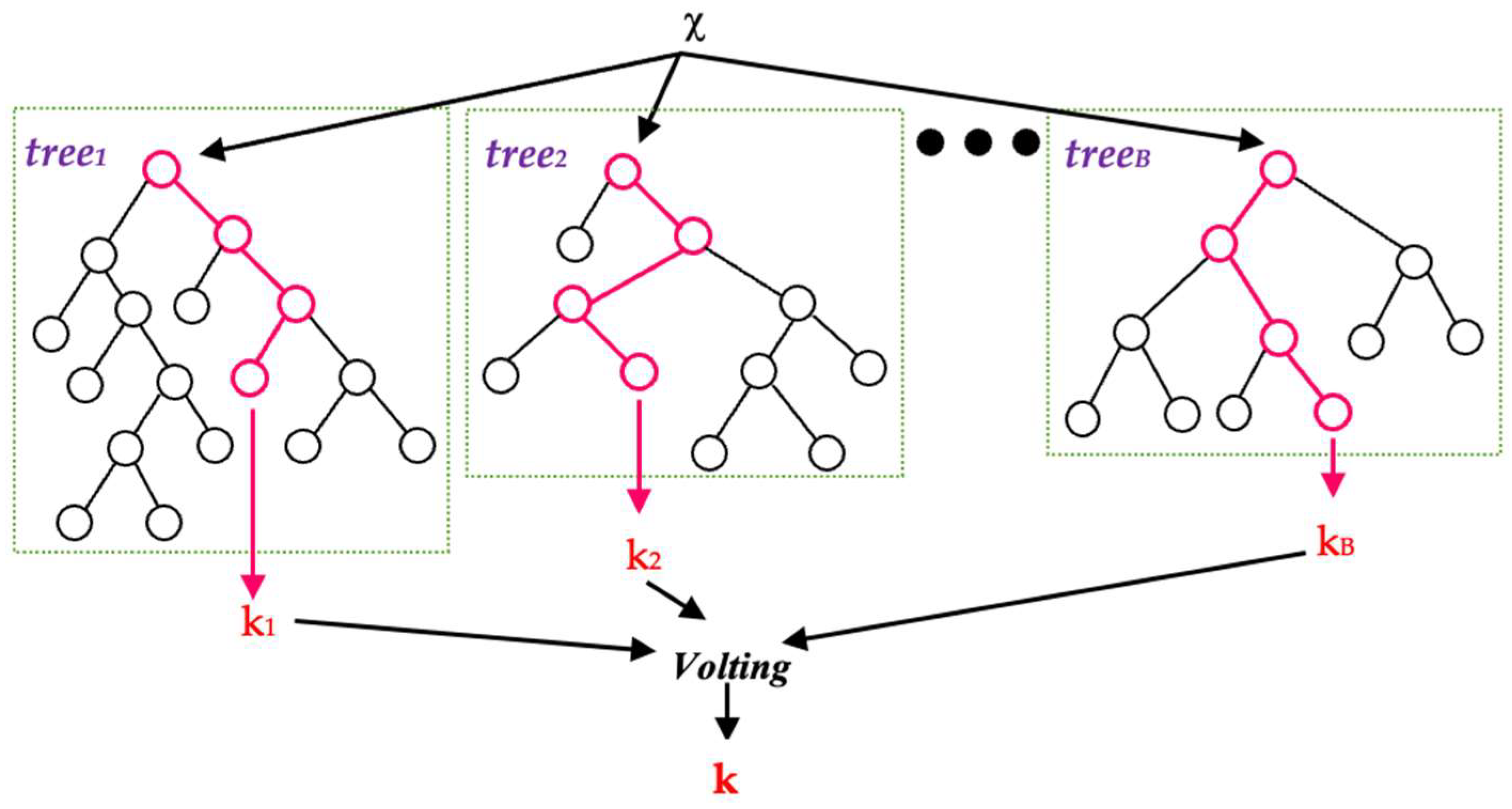
In the realm of machine learning, the random forest (RF) stands out as a widely embraced ensemble learning technique, frequently employed for tasks related to classification and regression (Figure 2). The essence of ensemble learning lies in combining predictions from multiple machine learning models to enhance forecast accuracy and reliability.

Contrary to linear regression, which assumes data linearity, random decision trees within the RF framework demonstrate superior predictive capabilities by swiftly adapting to non-linearities inherent in the data. While the simplicity of linear regression aids in model comprehension, it often falls short in predictive performance due to its reliance on the linearity assumption. Random forests exhibit enhanced prediction accuracy, particularly on medium to large datasets, as they effectively navigate and capture non-linear patterns.

In situations where the number of independent variables surpasses the number of observations, logistic regression and linear regression algorithms encounter limitations since there are more parameters to estimate than available data points. The random forest circumvents this constraint by selectively utilizing predictor variables, ensuring effective model performance [30].

The predictive process of the random forest model involves computing a forecast through the averaging of projections derived from individual decision trees. This aggregation mitigates model variance and contributes to an overall improvement in predictive accuracy [31].

Here is a detailed description of how a random forest model works:

• Divide the training data into different groups. The process used for this is called bagging.
• Use each subset of training data to train a decision tree. Only a random subset of features is considered at each split in the decision tree.
• Repeat steps 1 and 2 to create a forest of the decision tree.
• To predict something, take the average of all the projections from all the individual decision trees.

4.3. Support Vector Machine (SVM)

Another kernel-based machine learning approach employed for classification tasks and regression challenges is the support vector machine (SVM), pioneered by Vapnik in 1986 (Figure 3). This method is particularly utilized in support vector regression (SVR) to address regression problems. Successful applications of support vector machines in time series forecasting have been documented [24].

The SVM technique partitions data points into two classes with the widest margin by identifying a hyperplane within the input space. The margin represents the separation between the nearest data points for each class and the hyperplane. The hyperplane is determined through the resolution of a quadratic programming problem. A set of support vector data points closest to the hyperplane provides the solution to this problem. Once the support vectors are identified, new data points can be classified using SVM by projecting them onto the hyperplane. If data points lie on one side of the hyperplane, they are classified into a specific class; otherwise, they are grouped into the opposing class. SVMs are a potent machine learning technique applicable to regression and classification tasks, particularly effective with high-dimensional data and data exhibiting non-linear relationships [32,33].

The primary objective of model classification is to construct a model that performs optimally based on the training dataset. Conventional training methods often result in models that accurately memorize each input-output combination, leading to a decreased ability to generalize if the model is overly tailored to the training data. Conversely, SVM aims to categorize classes within the training set into as many distinct groups as possible using a surface that maximizes the separation between them. In essence, SVM facilitates the maximization of a model’s generalization potential [34].

4.4. XGBoost (XGB)

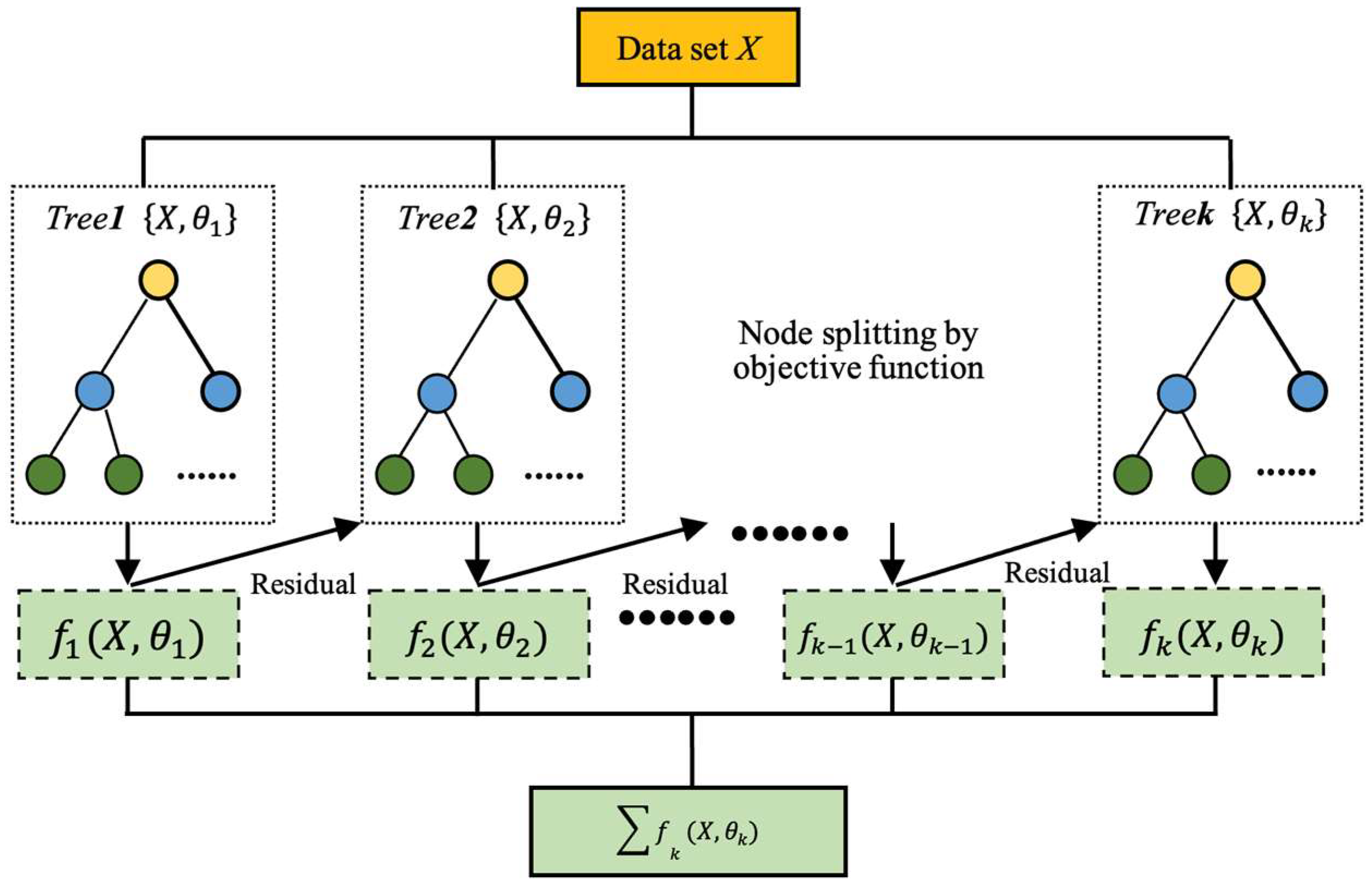
XGBoost (XGB) is a collection of decision trees based on gradient boosting, known for its high scalability (Figure 4). It achieves incremental expansion of the objective function by minimizing a loss attributed to gradient ascent. XGBoost utilizes a distinct loss function designed specifically for decision trees, the sole base classifiers employed in XGBoost. To expedite the training of decision trees without compromising ensemble accuracy, XGBoost implements various techniques. XGBoost addresses the computational complexity of decision tree construction, particularly the time-consuming step of determining optimal distribution. It targets this by optimizing the split search process. While conventional split search algorithms explore all potential candidate splits and choose the one with the highest gain, XGBoost streamlines this process by pre-sorting and storing data in a compressed column format. This reduces the need for repeated sorting at each node, ensuring each feature is sorted only once. Moreover, XGBoost incorporates randomization strategies to improve training efficiency and prevent overfitting. Random subsamples are employed during the training of individual trees, and column subsampling is applied at both the tree and tree node levels as part of XGBoost’s randomization approaches [35].

Each decision tree has learned to predict the residual error of the previous tree. The disparity between the actual target value and the predicted value of the previous tree is called residual error. The XGBoost algorithm uses a method known as gradient boosting to train decision trees. One additional decision tree is added to the set at a time using the iterative gradient boosting approach. Each new decision tree undergoes training to reduce the residual error of the previous trees. Other methods, such as regularization and early stopping, are also used by the XGBoost algorithm to improve model performance [36,37,38].

4.4.1. Case Study

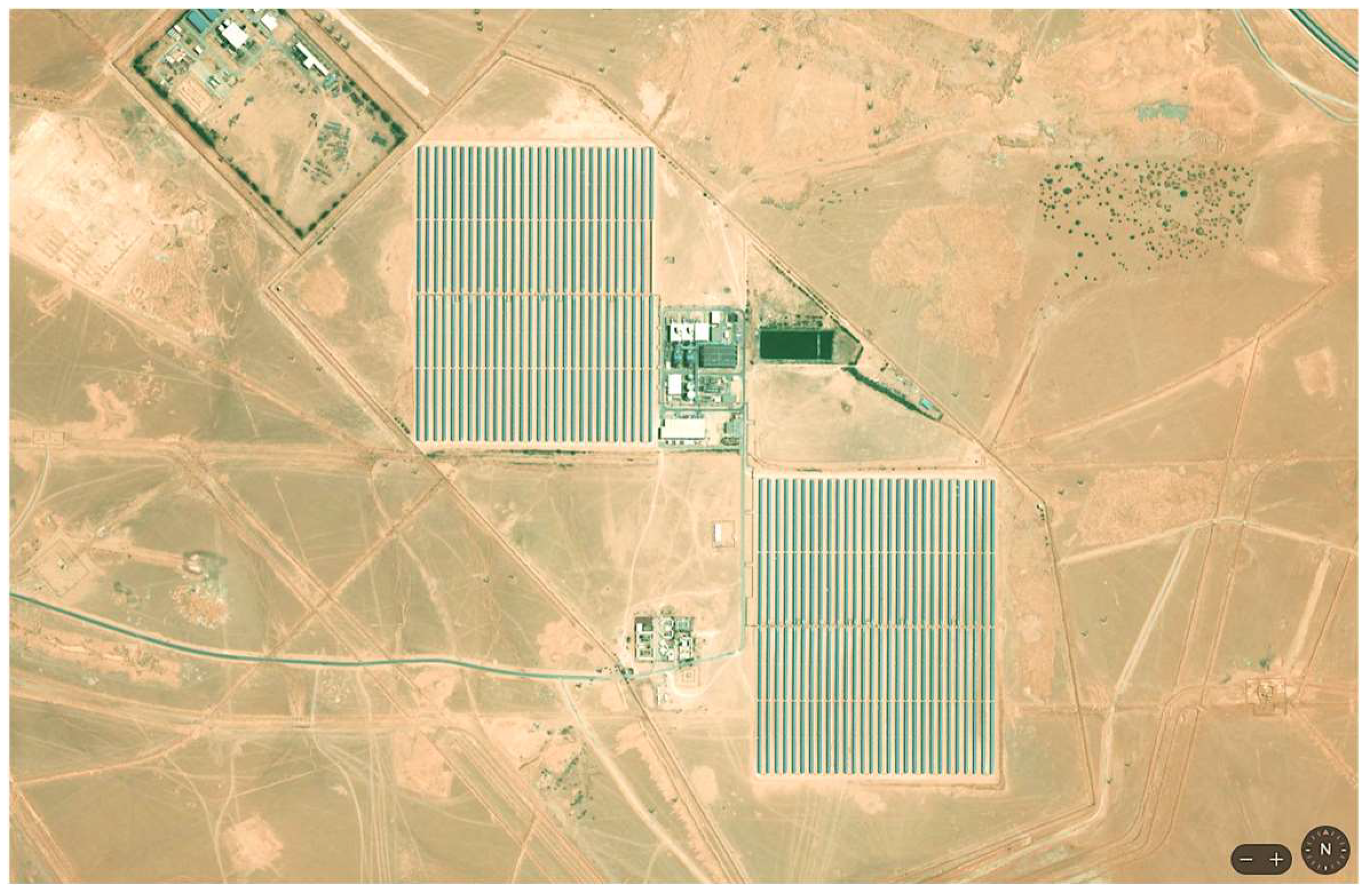
In this case study, a dataset containing historical information on the energy production of a solar farm located in Hassi R’mel, Laghouat, is used, Algeria (Latitude: 33°7′29.728″ N; Longitude: 3°21′22.484″ E). Figure 5 shows a satellite image of the Hassi R’Mel power plant.

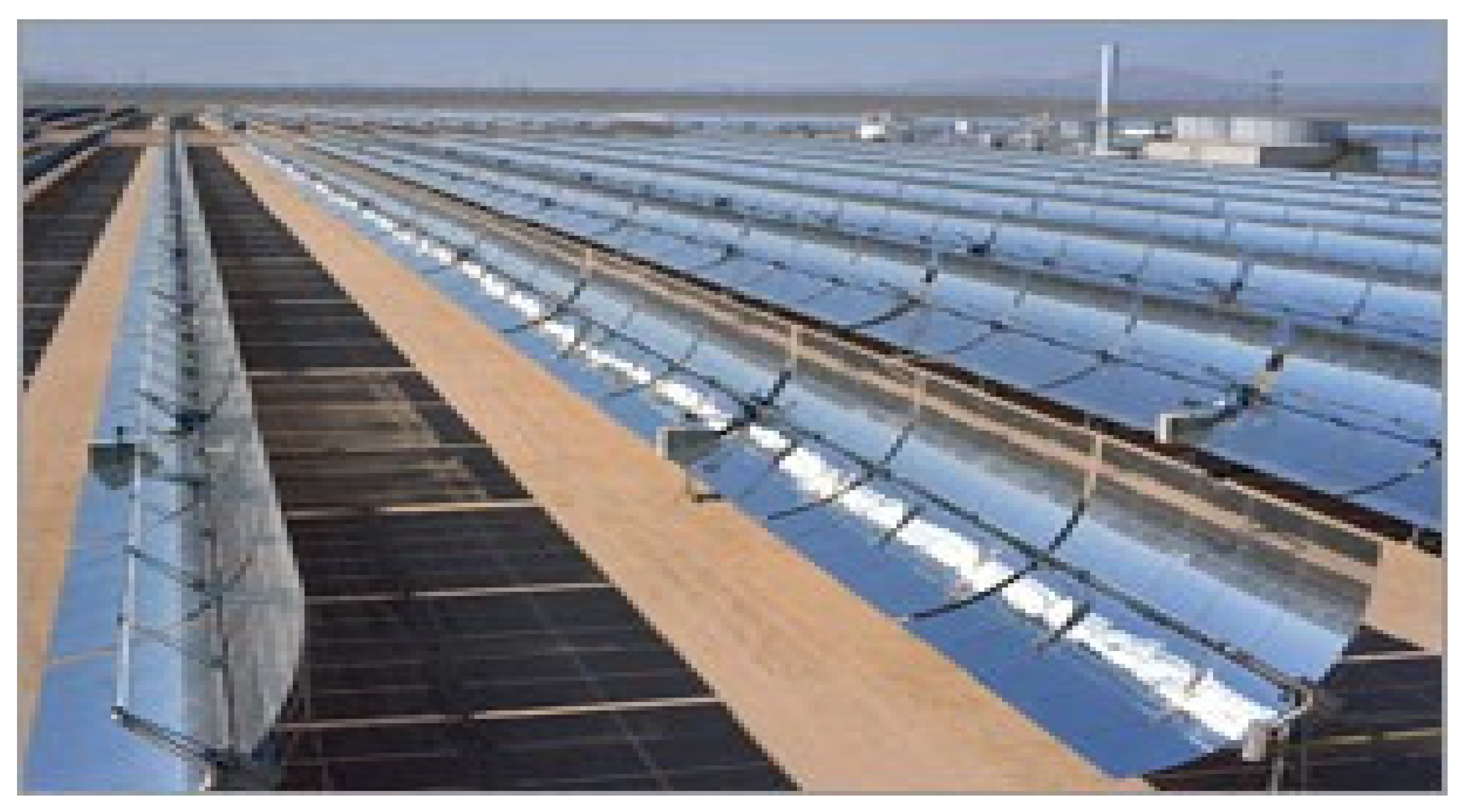
The Hassi R’Mel power installation, boasting a capacity of 150 MW, stands as a pioneering facility in the realm of thermo-solar and combined cycle hybrid electricity generation. Positioned within the largest natural gas field in Algeria, Hassi R’Mel, the installation incorporates two (02) gas turbines (40 MW), two 75 MW combustion systems, a steam turbine with a capacity of 80 MW, and two (02) parabolic solar fields contributing 25 MW to the production capacity. The solar fields encompass 224 parabolic collectors organized into 56 loops across an expansive area of 180,000 m². Figure 6 provides a visual representation, showcasing the power plant adorned with its distinctive parabolic-shaped collectors.

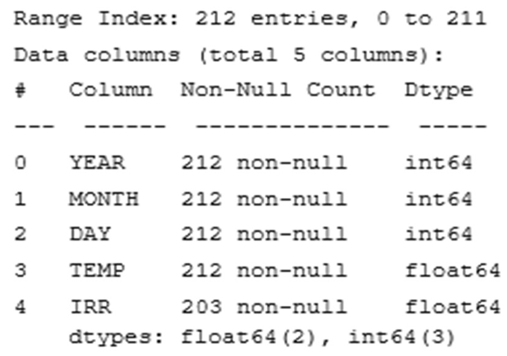
Historical data for temperatures and solar irradiance were collected daily from solar stations [39], covering a 7-month period from January to July (comprising 212 entries indexed from 0 to 211, each containing five columns: year, month, day, temperature, and irradiance).

The dataset is pre-processed by handling missing values and extracting relevant temporal features. The data used in this study are available at (Figure 7):

• NASA/POWER CERES/MERRA2 Native Resolution Daily Data
• Dates (month/day/year): 1 January 2023 through 31 April 2023
• Location: Longitude 3.356; Latitude 33.125;

Data may disappear due to file loss, equipment malfunction, or other reasons. This can reduce the statistical power of the analysis, making it less likely that true effects or relationships will be detected because missing data may be systematically related to the variables of interest. As shown in the table above, which was extracted from the program via Python, no value is lost as a result of processing the data used in this study (non-null).

In this study, the four models are employed for temperature and solar irradiance forecasting, with “YEAR”, “MONTH”, and “DAY” serving as design variables across all models. The decision tree model dynamically adapts its structure during training, utilizing a decision tree regressor with default parameters. The random forest model, employing the random forest regressor, determines its structure based on the number of trees and their configurations. The support vector machine (SVM) with a linear kernel characterizes its structure with the optimal hyperplane during training. In contrast, the XGBoost model utilizes the XGBoost Regressor with specific hyperparameters, including n_estimators = 100, learning_rate = 0.1, and max_depth = 3. All models share temporal features as input measures, offering predictions for temperature and solar irradiance.

Figure 8 illustrates the variations in temperature and solar irradiance throughout the month of January. The daily values represent the averages recorded per day, explaining the temperature drop of up to 2 °C during the first months, as observed in Figure 8.

4.4.2. Model Evaluation

The performance evaluation of each model involved the use of key metrics, including mean absolute error (MAE), mean squared error (MSE), and root mean square error (RMSE). The definitions of these metrics are provided using Equations (1)–(3), respectively, as outlined in the pertinent literature [26,27,39].

$$MAE=\frac{1}{N}{\sum }_{i=1}^N|{\hat{\mathrm{x}}}_i-{\mathrm{x}}_i|$$

(1)

$$MSE=\frac{1}{N}{\sum }_{i=1}^N{({\hat{\mathrm{x}}}_i-{\mathrm{x}}_i)}^2$$

(2)

$$RMSE=\sqrt{\frac{1}{N}{\sum }_{i=1}^N{({\hat{\mathrm{x}}}_i-{\mathrm{x}}_i)}^2}$$

(3)

Here, “N” represents the length of the time series, “${\hat{\mathrm{x}}}_i$” denotes the forecasted value, and “${\mathrm{x}}_i$” represents the measured value.

5. Discussion of Results

The initial section of the verification results focuses on visual comparison to evaluate the concordance between actual and predicted values within the test data for irradiance and temperature predictions. Moreover, quantitative evaluation employs metrics such as mean absolute error (MAE), mean squared error (MSE), and root mean square error (RMSE). Moving to the next section, the comparison of models expands to encompass various criteria, including complexity level, stability, response time, and implementation complexity. This multifaceted evaluation aims to offer a comprehensive understanding of the models’ performance beyond numerical metrics alone.

5.1. Temperature Prediction

The accuracy of temperature forecasts is contingent upon several factors, including the chosen forecast method, the quality of input data, and the complexity of prevailing weather conditions. Machine learning algorithms prove effective by being trained on extensive datasets comprising historical temperature data, which may encompass information from extreme weather events. This training enables algorithms to discern patterns and relationships associated with diverse climatic scenarios. Once trained, these algorithms exhibit the capability to provide more precise predictions about future temperatures, even when faced with conditions beyond the range of historical data. In the specific case outlined, the program leverages data spanning several months to enhance its training, capturing the nuances of climate changes throughout different seasons. 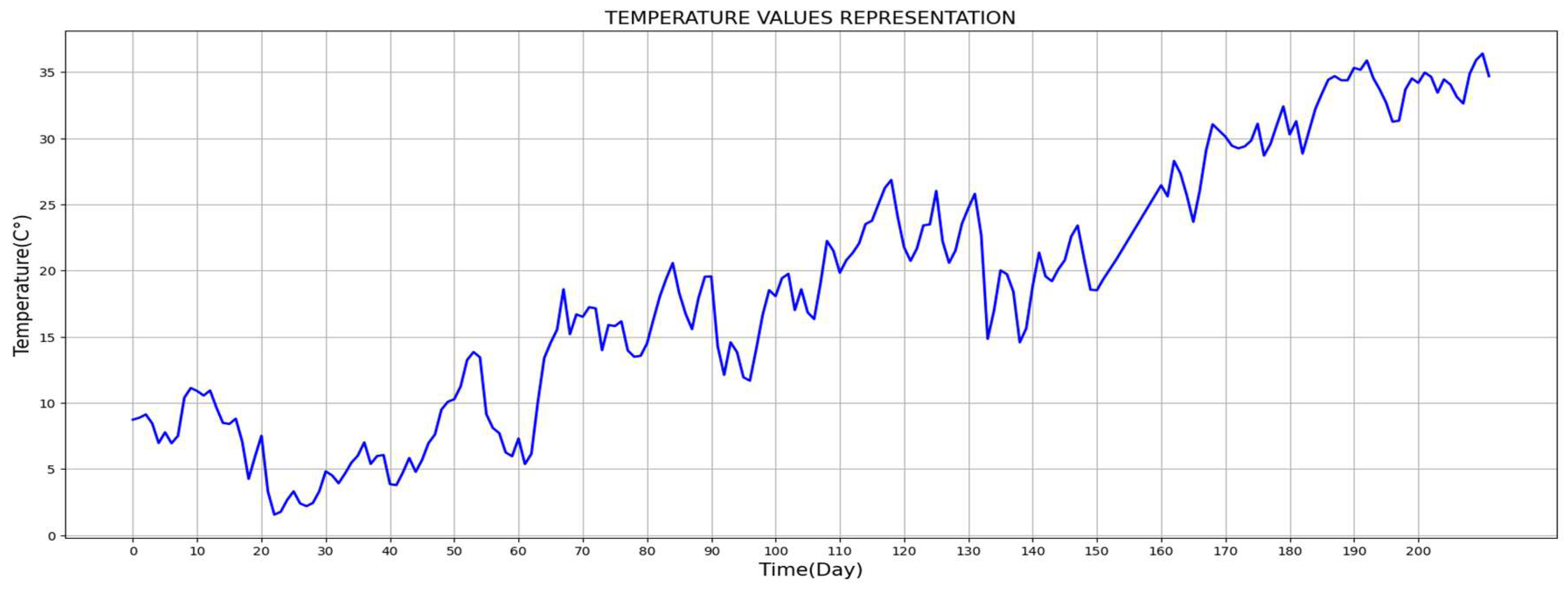Figure 9 visually represents the variation in temperature within the study area over a duration of seven months.

Note

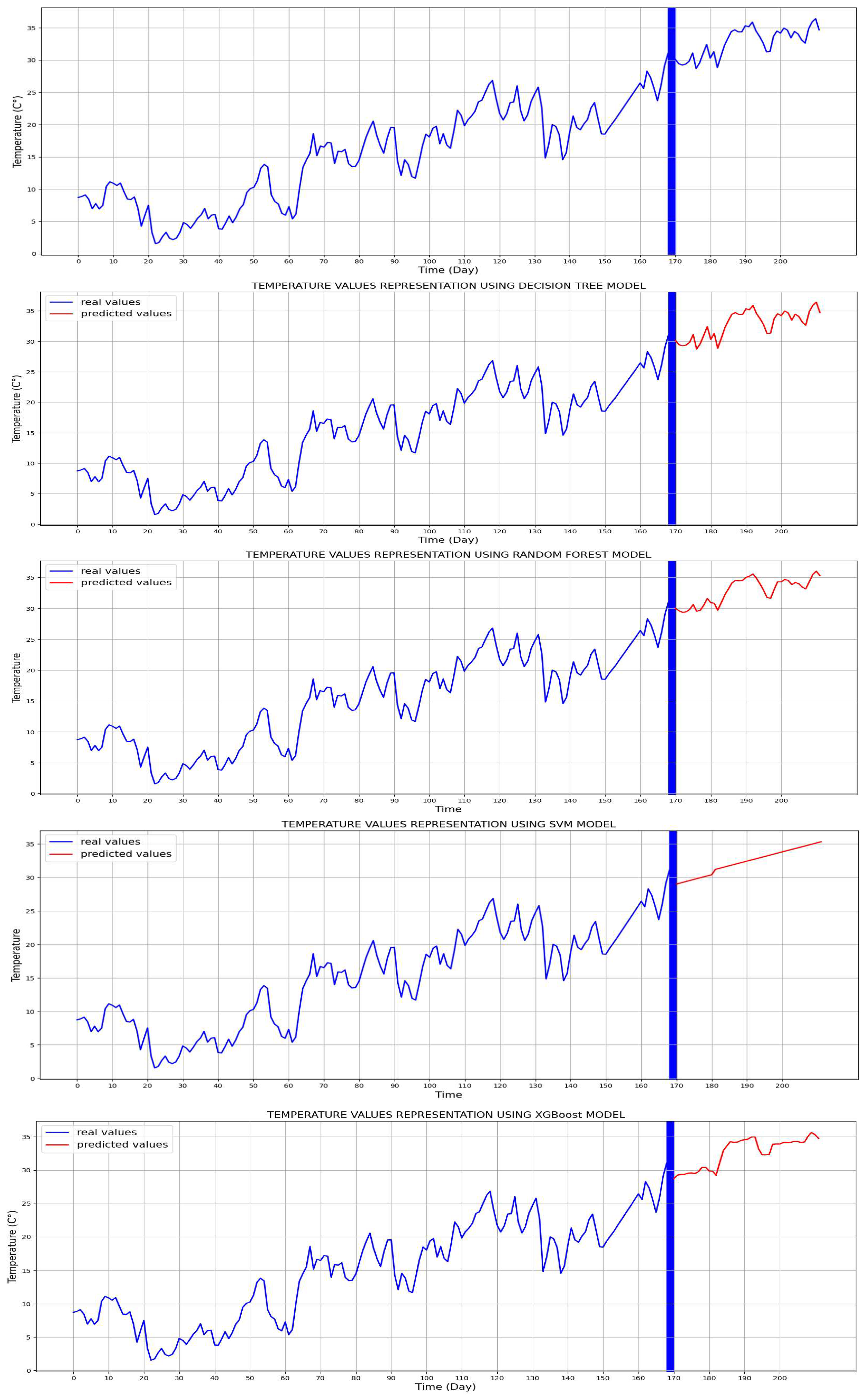
In this process, the decision tree model registers a value of 0 in the metrics, signifying that the studied model perfectly fits the training data. This exceptional case implies that the model attains flawless accuracy in predicting the values of the target variable for all training data points. Such a scenario is uncommon and is more likely to occur with smaller training datasets. In this instance, 80% of the data is allocated for the model training, corresponding to 167 days. Figure 10 provides a visual comparison of the predicted temperature values among the four models, highlighting the distinctive characteristics and performance of each. For each studied model, the values of the MAE, MSE, and RMSE for temperature forecasting are shown in

Table 4. The values of metrics for temperature forecasting.

Model	MAE	MSE	RMSE
DT	0.00000 *	0.00000 *	0.00000 *
RF	0.32031	0.15355	25.15817
SVM	1.18382	2.25412	24.38985
XGBoost	0.59879	0.58510	0.76492

* Raw result obtained from data treatment.

.

5.2. Solar Irradiance Prediction

Solar irradiation forecasting involves the complex process of predicting how much sunlight will reach a specific location at a given time in the future. However, this process has become more complex due to ongoing climate change. As the planet warms, we observe an increase in extreme weather events, such as thick clouds and dust storms, which are becoming more frequent. These extreme weather conditions can significantly reduce the amount of sunlight reaching the Earth’s surface, making it extremely difficult to predict solar irradiation levels accurately.

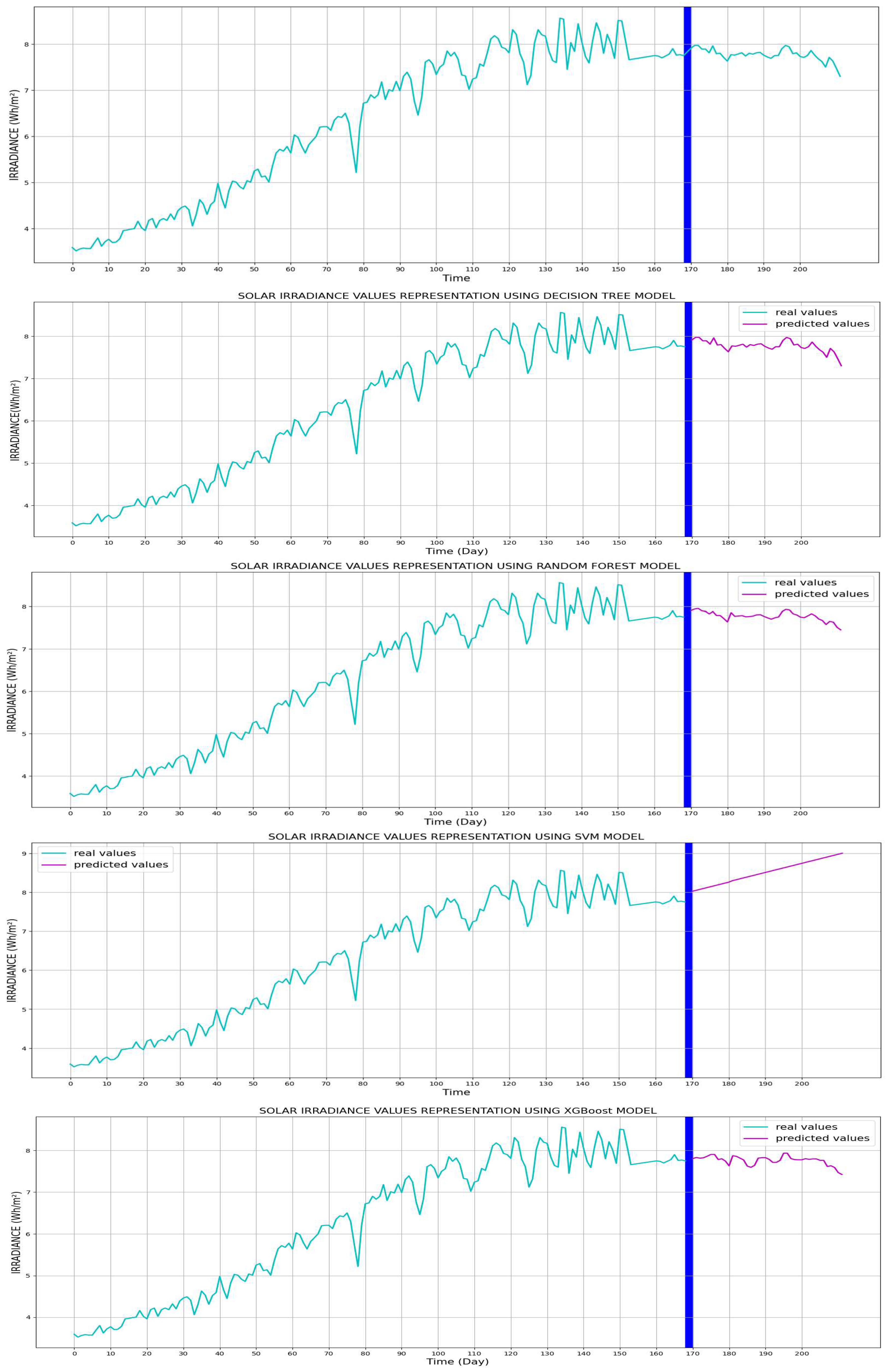
This increased complexity explains the relatively low solar irradiation scores recorded during the first months of the study. Figure 11, shown above, provides a visual overview of the collected solar irradiation data, highlighting the challenges of forecasting this vital resource. Figure 12 illustrates a comparison between the different models for predicted irradiance values. Values of MAE, MSE, and RMSE for solar irradiance forecasting are presented in

Table 5. The values of metrics for solar irradiance forecasting.

Model	MAE	MSE	RMSE
DT	0.00000 *	0.00000 *	0.00000 *
RF	0.02702	0.027029	0.03940
SVM	0.75297	0.75297	0.84729
XGBoost	0.06601	0.06601	0.08301

* Data raw result obtained from data treatment, a decision tree works by recursively splitting the data based on the features, creating decision nodes to differentiate between different classes (in this case, we are concerned with regression, not classification, as such we are not going to work with classes). Thus, achieving 0 error in a DT model is theoretically possible, especially if you have a small and well-structured dataset.

.

5.2.1. Interpretation

In this study, the models underwent training with the exclusion of the last 40 days that were selected for the test set. Upon evaluation of its accuracy, the SVM model emerged with the highest mean absolute error (MAE) value, indicating its relatively weaker performance compared to the other models. The XGBoost model secured the second position, followed by the RF model, with the simple DT model ranking last. Graphical analysis unveiled that the representation of temperature values generated by the decision tree model closely resembled the original representation. This observation implies that the decision tree model retained the fundamental characteristics of the original data, offering valuable insights into temperature patterns within the study.

5.2.2. Measuring Forecast Speed

The forecasting speed of a model varies depending on the model architecture, the size of the dataset, and the hardware the model is running on. However, measuring forecast speed can be useful for comparing different models or for optimizing a model’s performance. As we can see in

Table 6. The values of forecasting speed (s).

Model	DT	RF	SVM	XGB
Temperature	0.00588	0.01296	0.01292	0.00199
Irradiance	0.00399	0.02592	0.00793	0.00426

, both DT and XGB achieve a low prediction speed (unit is second).

Table 7. Comparison of the different models using other factors.

Model	Complexity	Speed	Efficiency
DT	Simple	Very fast	More efficient
RF	Simple	Fairly fast	Efficient
SVM	Simple	Fairly fast	Not enough
XGB	Medium	Very fast	Efficient

presents a comparison between different models according to their complexity of implementation, their speed, and their efficiency.

The evaluation results indicate that the decision tree stands out as an accurate and robust forecasting tool for both temperature and solar irradiance. The model demonstrates the capability to achieve low mean absolute error (MAE), mean squared error (MSE), and root mean square error (RMSE) values, along with optimal forecasting speed. However, the selection of the most suitable forecasting model is contingent on the specific requirements of the application. In the current study, where forecasting accuracy and speed are paramount, the decision tree model excels on both fronts. Decision trees exhibit high accuracy by adeptly learning intricate relationships between features and the target variable. Through recursive data division based on feature values, decision trees discern complex patterns, contributing to their accurate predictions.

Decision trees are notably fast due to their avoidance of complex calculations. The algorithm’s efficiency lies in comparing the feature values of a data point with those of the training data and, upon finding a match, assigning a label to the data point. Moreover, decision trees showcase versatility by accommodating both continuous and categorical features, rendering them a versatile and adaptable machine-learning algorithm for various applications.

Differential privacy techniques provide a robust framework for injecting controlled noise into the training process, thereby protecting individual data points such as federated learning and homomorphic encryption. By integrating these advanced privacy-preserving techniques, our future research aims to strike a delicate balance between accuracy, model complexity, and computational efficiency, thereby contributing to the development of secure and privacy-friendly ML models for predicting energy production photovoltaic. By exchanging model parameters rather than private data, the intended FedDRL (federated deep reinforcement learning) can produce an accurate prediction model in a decentralized manner, thus avoiding sensitive privacy issues [40]. Moreover, homomorphic encryption (HE), with its security guarantees and computability on encrypted data, has become one of the most promising techniques to protect data privacy [41]. This proactive approach aligns with the evolving data protection landscape and highlights our commitment to ensuring responsible and ethical use of energy-related data in the context of renewable energy forecasting.

6. Conclusions

In this paper, four ML algorithms were designed to predict future temperature and irradiance values with high accuracy: decision tree, support vector machine, random forest, and XGBoost.

The effectiveness of these methods was evaluated based on different simulation studies. A comparative study between these algorithms is presented according to three parameters: the mean absolute error, the absolute error, and the mean square error.

Based on the results, the present study highlights the importance of accurate temperature and solar irradiation estimates to optimize photovoltaic systems. The simple decision tree algorithm allows the model to make predictions very quickly. However, it is important to note that the accuracy of a decision tree model depends on the quality of the training data and the choice of features. We also propose using ensemble methods like gradient boosting to improve accuracy in photovoltaic energy production forecasting. These methods combine multiple models for higher accuracy while remaining computationally efficient. They also recommend streamlining model complexity by focusing on relevant features, using techniques like recursive feature elimination (RFE) or feature importance analysis. Additionally, fine-tuning model hyperparameters is crucial for finding the right balance between accuracy and efficiency. On another note, researchers emphasize advanced feature engineering to capture nuanced relationships in meteorological data for better accuracy, particularly in the context of climate change-induced variability. Integrating climate models into forecasting processes helps understand long-term climate trends, and real-time data assimilation techniques enhance accuracy amidst climate variability by continuously incorporating the latest observational data. These strategies effectively manage tradeoffs in forecasting accuracy, model complexity, and computational efficiency in photovoltaic energy production.

By providing the tools needed for efficient and sustainable solar energy production, machine learning models, particularly decision trees, have the potential to transform the energy sector. Furthermore, given the self-adaptive nature of ML models, this article can be used as a reference because the results mentioned can be considered sustainable.

Concerning our future research on forecasting photovoltaic energy production, this study will be developed subsequently via other machine learning models and, in particular, on the improvement of model architectures, the search for new approaches, and the integration of technology techniques to improve forecast accuracy. The results of this study pave the way for better consumption of renewable energies in areas rich in solar resources.

The results obtained in this article make a notable contribution to the field of photovoltaic energy production forecasting by shedding light on the choice of predictive models used in the development of solar energy infrastructures in order to obtain forecasts. They are more accurate and reliable for efficient energy management and predicting energy and financial gains.

References

- Mierzwiak, M.; Kroszczyński, K. Impact of Domain Nesting on High-Resolution Forecasts of Solar Conditions in Central and Eastern Europe. Energies 2023, 16, 4969. [Google Scholar] [CrossRef]
- Wolniak, R.; Skotnicka-Zasadzień, B. Development of Photovoltaic Energy in EU Countries as an Alternative to Fossil Fuels. Energies 2022, 15, 662. [Google Scholar] [CrossRef]
- Yagli, G.M.; Yang, D.; Srinivasan, D. Reconciling solar forecasts: Sequential reconciliation. Sol. Energy 2019, 179, 391–397. [Google Scholar] [CrossRef]
- Mellit, A.; Massi Pavan, A.; Ogliari, E.; Leva, S.; Lughi, V. Advanced Methods for Photovoltaic Output Power Forecasting: A Review. Appl. Sci. 2020, 10, 487. [Google Scholar] [CrossRef]
- Wan, C.; Zhao, J.; Song, Y.; Xu, Z.; Lin, J.; Hu, Z. Photovoltaic and solar power forecasting for smart grid energy management. IEEE CSEE J. Power Energy Syst. 2015, 1, 38–46. [Google Scholar] [CrossRef]
- Lima, M.A.F.B.; Carvalho, P.C.M.; Fernandez-Ramírez, L.M.; Braga, A.P.S. Improving solar forecasting using deep learning and portfolio theory integration. Energy 2020, 195, 117016. [Google Scholar] [CrossRef]
- Tian, J.; Ooka, R.; Lee, D. Multi-scale solar radiation and photovoltaic power forecasting with machine learning algorithms in urban environment: A state-of-the-art review. J. Clean. Prod. 2023, 426, 139040. [Google Scholar] [CrossRef]
- Sharma, A.; Kakkar, A. Forecasting daily global solar irradiance generation using machine learning. Renew. Sustain. Energy Rev. 2018, 82, 2254–2269. [Google Scholar] [CrossRef]
- Zhou, Y. Advances of Machine Learning in Multi-Energy District Communities—Mechanisms, Applications and Perspectives. Energy AI 2022, 10, 100187. [Google Scholar] [CrossRef]
- Gheibi, O.; Weyns, D.; Quin, F. Applying machine learning in self-adaptive systems: A systematic literature review. ACM Trans. Auton. Adapt. Syst. 2021, 15, 1–37. [Google Scholar] [CrossRef]
- Denholm, P.; Margolis, R.M. Evaluating the limits of solar photovoltaics (PV) in traditional electric power systems. Energy Policy 2007, 35, 2852–2861. [Google Scholar] [CrossRef]
- Adewuyi, O.B.; Lotfy, M.E.; Olabisi Akinloye, B.; Howlader Hor, R.; Senjyu, T.; Narayanan, K. Security-constrained optimal utility-scale solar PV investment planning for weak grids: Short reviews and techno-economic analysis. Appl. Energy 2019, 245, 16–30. [Google Scholar] [CrossRef]
- Pérez-Arriaga, I.J.; Batlle, C. Impacts of Intermittent Renewables on Electricity Generation System Operation. Econ. Energy Environ. Policy 2012, 1, 3–18. [Google Scholar] [CrossRef]
- Batlle, C.; Rodilla, P. Generation Technology Mix, Supply Costs, and Prices in Electricity Markets with Strong Presence of Renewable Intermittent Generation 2011; IIT Working Paper IIT-11-020A; Institute for International Trade: Adelaide, Australia, 2011. [Google Scholar]
- Rehman, S.; Bader, M.A.; Al-Moallem, S.A. Cost of solar energy generated using PV panels. Renew. Sustain. Energy Rev. 2007, 11, 1843–1857. [Google Scholar] [CrossRef]
- Majdi, A.; Alqahtani, M.D.; Almakytah, A.; Saleem, M. Fundamental Study Related to The Development of Modular Solar Panel for Improved Durability and Repairability. IET Renew. Power Generation. (RPG) 2021, 15, 1382–1396. [Google Scholar] [CrossRef]
- Wang, G.; Su, Y.; Shu, L. One-day-ahead daily power forecasting of photovoltaic systems based on partial functional linear regression models. Renew Energy 2016, 96, 469–478. [Google Scholar] [CrossRef]
- Khan, H.A.; Alam, M.; Rizvi, H.A.; Munir, A. Solar Irradiance Forecasting Using Deep Learning Techniques. Eng. Proc. 2023, 46, 15. [Google Scholar] [CrossRef]
- Kumar, D.S.; Yagli, G.M.; Kashyap, M.; Srinivasan, D. Solar irradiance resource and forecasting: A comprehensive review. IET 2020, 14, 1641–1656. [Google Scholar] [CrossRef]
- Ramirez-Vergara, J.; Bosman, L.B.; Leon-Salas, W.D.; Wollega, E. Ambient temperature and solar irradiance forecasting prediction horizon sensitivity analysis. Mach. Learn. Appl. 2021, 6, 100128. [Google Scholar] [CrossRef]
- Cotfas, D.T.; Marzband, M.; Cotfas, P.A.; Siroux, M.; Sera, D. Editorial: Forecasting solar radiation, photovoltaic power and thermal energy production applications. Front. Energy Res. 2022, 10, 1115096. [Google Scholar] [CrossRef]
- Rahimi, N.; Park, S.; Choi, W.; Oh, B.; Kim, S.; Cho, Y.H.; Ahn, S.; Chong, C.; Kim, D.; Jin, C.; et al. A Comprehensive Review on Ensemble Solar Power Forecasting Algorithms. J. Electr. Eng. Technol. 2023, 18, 719–733. [Google Scholar] [CrossRef]
- Alkabbani, H.; Ahmadian, A.; Zhu, Q.; Elkamel, A. Machine Learning and Metaheuristic Methods for Renewable Power Forecasting: A Recent Review. Front. Chem. Eng. 2021, 3, 665415. [Google Scholar] [CrossRef]
- Voyant, C.; Notton, G.; Kalogirou, S.; Nivet, M.L.; Paoli, C.; Motte, F.; Fouilloy, A. Machine learning methods for solar radiation forecasting: A review. Renew. Energy 2017, 105, 569–582. [Google Scholar] [CrossRef]
- Yang, B.; Zhu, T.; Cao, P.; Guo, Z.; Zeng, C.; Li, D.; Chen, Y.; Ye, H.; Shao, R.; Shu, H.; et al. Classification and Summarization of Solar Irradiance and Power Forecasting Methods: A Thorough Review. CSEE J. Power Energy Syst. 2023, 9, 978–995. [Google Scholar] [CrossRef]
- Van Der Meer, D.W.; Widén, J.; Munkhammar, J. Review on probabilistic forecasting of photovoltaic power production and electricity consumption. Renew. Sustain. Energy Rev. 2018, 81, 1484–1512. [Google Scholar] [CrossRef]
- Okumus, I.; Dinler, A. Current status of wind energy forecasting and a hybrid method for hourly predictions. Energy Convers. Manag. 2016, 123, 362–371. [Google Scholar] [CrossRef]
- Rokach, L.; Maimon, O. Decision Trees. In Data Mining and Knowledge Discovery Handbook; Springer: Berlin/Heidelberg, Germany, 2006; pp. 165–192. [Google Scholar]
- Song, Y.Y.; Lu, Y. Decision tree methods: Applications for classification and prediction. Shanghai Arch Psychiatry 2015, 27, 130–135. [Google Scholar] [CrossRef] [PubMed]
- Schonlau, M.; Zou, R.Y. The random forest algorithm for statistical learning. Stata J. 2020, 20, 3–29. [Google Scholar] [CrossRef]
- Breiman, L. Random Forests. Mach. Learn. 2001, 45, 5–32. [Google Scholar] [CrossRef]
- Pisner, D.A.; Schnyer, D.M. Support vector machine. In Machine Learning: Methods and Applications to Brain Disorders; Elsevier: Amsterdam, The Netherlands, 2019; pp. 101–121. [Google Scholar]
- Jun, Z. The Development and Application of Support Vector Machine. Stata J. Promot. Commun. Stat. Stata 2020, 20, 3–29. [Google Scholar] [CrossRef]
- Cervantes, J.; Garcia-Lamont, F.; Rodríguez-Mazahua, L.; Lopez, A. A comprehensive survey on support vector machine classification: Applications, challenges and trends. Neurocomputing 2020, 408, 189–215. [Google Scholar] [CrossRef]
- Bentéjac, C.; Csörgő, A.; Martínez-Muñoz, G. A comparative analysis of XGBoost. Artif. Intell. Rev. 2021, 54, 1937–1967. [Google Scholar] [CrossRef]
- Chen, T.; Guestrin, C. XGBoost: A scalable tree boosting system. In Proceedings of the ACM SIGKDD International Conference on Knowledge Discovery and Data Mining, San Francisco, CA, USA, 13–17 August 2016; Association for Computing Machinery: New York, NY, USA, 2016; pp. 785–794. [Google Scholar]
- Sabri, M.; Hassouni, M. El: Photovoltaic Power Forecasting with a Long Short-Term Memory Autoencoder Networks. Soft Comput. 2022, 27, 10533–10553. [Google Scholar] [CrossRef]
- NASA. Prediction of Worldwide Energy Resources.: Power Data Access Viewer. 2023. Available online: https://power.larc.nasa.gov/data-access-viewer/ (accessed on 1 February 2024).
- Hu, T.; Song, T. Research on XGBoost academic forecasting and analysis modelling. J. Phys. Conf. Ser. 2019, 1324, 012091. [Google Scholar] [CrossRef]
- Li, Y.; Wang, R.; Li, Y.; Zhang, M.; Long, C. Wind power forecasting considering data privacy protection: A federated deep reinforcement learning approach. Appl. Energy 2023, 329, 120291. [Google Scholar] [CrossRef]
- Xu, W.; Sun, J.; Cardell-Oliver, R.; Mian, A.; Hong, J.B. A Privacy-Preserving Framework Using Homomorphic Encryption for Smart Metering Systems. Sensors 2023, 23, 4746. [Google Scholar] [CrossRef] [PubMed]
Figure 1.
An example of the decision tree model’s algorithm.
Figure 2.
An example of the random forest model’s algorithm.
Figure 3.
Schematic description of the SVM model algorithm.
Figure 4.
Example of XGBoost model’s algorithm.
Figure 5.
Satellite image of the Hassi R’Mel power plant.
Figure 6.
Parabolic Collector of the Power Plant.
Figure 7.
Description of data shown using Python.
Figure 8.
The dataset from the month of January in Hassi R’Mel used in this study is presented as follows: (Top) the daily average temperature recorded per day, (Bottom) the daily solar irradiance data for the month of January.
Figure 9.
Representation of the temperature data.
Figure 10.
Representation of the solar irradiance data.
Figure 11.
Comparison between different models for predicted temperature values.
Figure 12.
Comparison between the different models for predicted irradiance values.