The Development of a Reduced-Scale Laboratory for the Study of Solutions for Microgrids

Abstract

The integration of renewable energy sources is crucial for achieving sustainability and environmental preservation. However, their intermittent nature poses challenges to electrical system stability, requiring robust integration strategies. Microgrids emerge as a flexible solution, but their successful deployment requires meticulous planning and intelligent operation to overcome these challenges. This paper presents the development of a reduced-scale laboratory dedicated to researching both hardware and software solutions for intelligent microgrid management. The laboratory was designed to incorporate key components that are becoming increasingly important in the present microgrid context, including renewable energy generation, storage systems, electrolyzers for hydrogen production, and combined heat and power sources. While some equipment consists of commercial models, the battery bank, converter, and supervisory systems were custom-designed to meet the specific requirements of the laboratory. The laboratory has proven itself as a robust tool for conducting studies on microgrids, effectively incorporating essential components, addressing pertinent system issues, and allowing for several tests on converting control algorithms.

1. Introduction

The increasing integration of renewable energy sources is paramount in reshaping the energy landscape, providing a pivotal response to contemporary sustainability challenges. The utilization of RES, such as solar and wind resources, not only curbs greenhouse gas emissions but also diminishes reliance on fossil fuels. Moreover, this diversification of the energy mix bolsters supply security. However, the intermittent and stochastic characteristics intrinsic to RES exert profound ramifications on electrical system stability. Consequently, there emerges a demand to develop robust integration strategies capable of handling the innate variability and unpredictability of these sources [1,2].

Microgrids represent an innovative and strategic answer to the complexities stemming from the increasing integration of renewable energy sources into power grids. A microgrid constitutes a remarkably adaptable, dynamic, and manageable entity, encompassing microgeneration units that draw upon renewable energy sources or low-carbon technologies, serving combined heat and power functions, energy storage mechanisms, and diverse loads [3,4,5,6].

Nevertheless, this utopian vision is accompanied by challenges in the system control and management. These challenges encompass power allocation, power quality assurance, stability assurance, environmental considerations, and economic viability [7]. Achieving these objectives mandates not only meticulous planning and MG system design but also astute and intelligent operation of its constituent elements, while duly acknowledging practical considerations.

Designing an MG interface control strategy is a crucial topic to handle. An MG can function as either a grid-connected system or an island. However, utilities and current standards [8,9] prohibit the operation of MGs on islands. The primary reasons for deliberate islanding are safety concerns regarding the powered section of the utility system, as well as the complicated control, communication, and protection requirements [10,11].

The development of power electronics has rendered power converter-interfaced distributed generation units capable of furnishing dependable power provision to end-users, thereby facilitating the assimilation of sophisticated control algorithms [7]. This evolution forms a crucial facet of enabling the realization of MG objectives.

Furthermore, microgrids can function as innovations and experimental platforms for novel demand management tactics, grid control techniques, and the integration of communication technologies. The coordination of local resources within a microgrid, facilitated by adept controllers and communication systems, empowers the distribution-level power infrastructure with substantial autonomy. This autonomy not only makes the assimilation of intermittent renewable energy easier but also bestows microgrids with a proactive role in stabilizing and controlling the broader electricity system. In this capacity, microgrids serve as buffers, adeptly absorbing fluctuations in both generation and demand, thereby contributing to overall system stability and control [3,12,13].

To optimize microgrid operation, control techniques require communication networks or linkages between levels [14]. Create communication interfaces to offer bidirectional channels for information flow between controllers [15]. Data flow between nodes in both directions, with each node capable of receiving and sending data via links to other nodes or endpoints. Microgrid nodes give information and communication capabilities to dispersed energy resources, resulting in intelligent electronic devices (IEDs) [16]. The microgrid controller may interface with IEDs and other components to send data and control orders.

This article addresses a significant gap in current research by introducing a scaled-down laboratory for developing and testing hardware and software associated with power electronics-based devices in the context of microgrids. While contemporary studies predominantly focus on microgrids within the system and integration domain, there is a notable lack of emphasis on hardware and its potential applications in industrial settings.

Notably, in works by Rojas et al. [17] and Jabbar et al. [18], microgrid laboratories are presented where the supervisory system is implemented using LabVIEW 2019 software. In contrast, our developed supervisory system utilizes Elipse E3 (version 6) software, founded on the SCADA system. This choice facilitates more agile data acquisition and visualization, rendering it better suited for industrial applications. Furthermore, the licensing cost of Elipse is considerably lower than that of LabVIEW.

In other studies [13,19,20], complete microgrid laboratories are showcased, albeit with simulated hardware. Sbordone et al. [21] employ physical hardware but with low power capacity. To bridge the gap and bring the laboratory closer to a real-world scenario, we have developed/used hardware with power levels closely resembling real-world situations on a small scale.

In line with the growing trend towards hydrogen as a clean fuel, our laboratory setup incorporates an electrolyzer in an alkaline environment to explore its integration into microgrids. Given the ongoing consolidation of this scenario, there is a scarcity of literature addressing the specific challenges and considerations related to the incorporation of electrolyzers into microgrids.

Laboratories such as Merabet et al. [22], Akpolat et al. [23], and Patel et al. [24] introduce microgrid laboratories featuring electrolyzers in their setups. However, these systems typically exhibit topologies with sets of renewable sources and electrolysis units connected in a common DC system—a configuration not conventional in an industrial context. To enhance the scalability of these systems for real-world installations, a strategic decision was made to connect the majority of these DC-based components to an AC bus through dedicated converters.

This AC-oriented approach provides a platform for studying the impacts on specific loads, such as electrolyzers, in terms of power quality. Moreover, it enables the development of hardware and software devices geared towards mitigating potential issues associated with these components, thereby addressing critical aspects of their integration into microgrids.

The majority of publications focusing on microgrid laboratories typically take into consideration more conventional renewable sources such as wind generators and photovoltaic arrays. Consequently, certain promising generation and cogeneration technologies are often overlooked despite their considerable potential. Our laboratory endeavors to broaden this perspective by integrating non-traditional cogeneration sources, such as the thermoelectric generator (TEG) system. The TEG system is founded on harnessing thermal energy expelled in industrial microgrids or generator plants, as seen in thermoelectric power stations. The inclusion of these less conventional sources in the laboratory setting aims to enhance our understanding and refinement of hardware systems and algorithms. This approach is geared towards improving overall efficiency while fostering a more synergistic integration with microgrid structures and their diverse energy demands.

The paper is organized as follows: Section 2 introduces the equipment used in the laboratory. Section 3 presents the control loops pertinent to the devised converters. Section 4 presents the results associated with the operation of the laboratory with special attention to the non-commercial devices that were developed. Finally, Section 5 concludes the paper and presents suggestions for future work.

2. Description of the Reduced-Order Laboratory

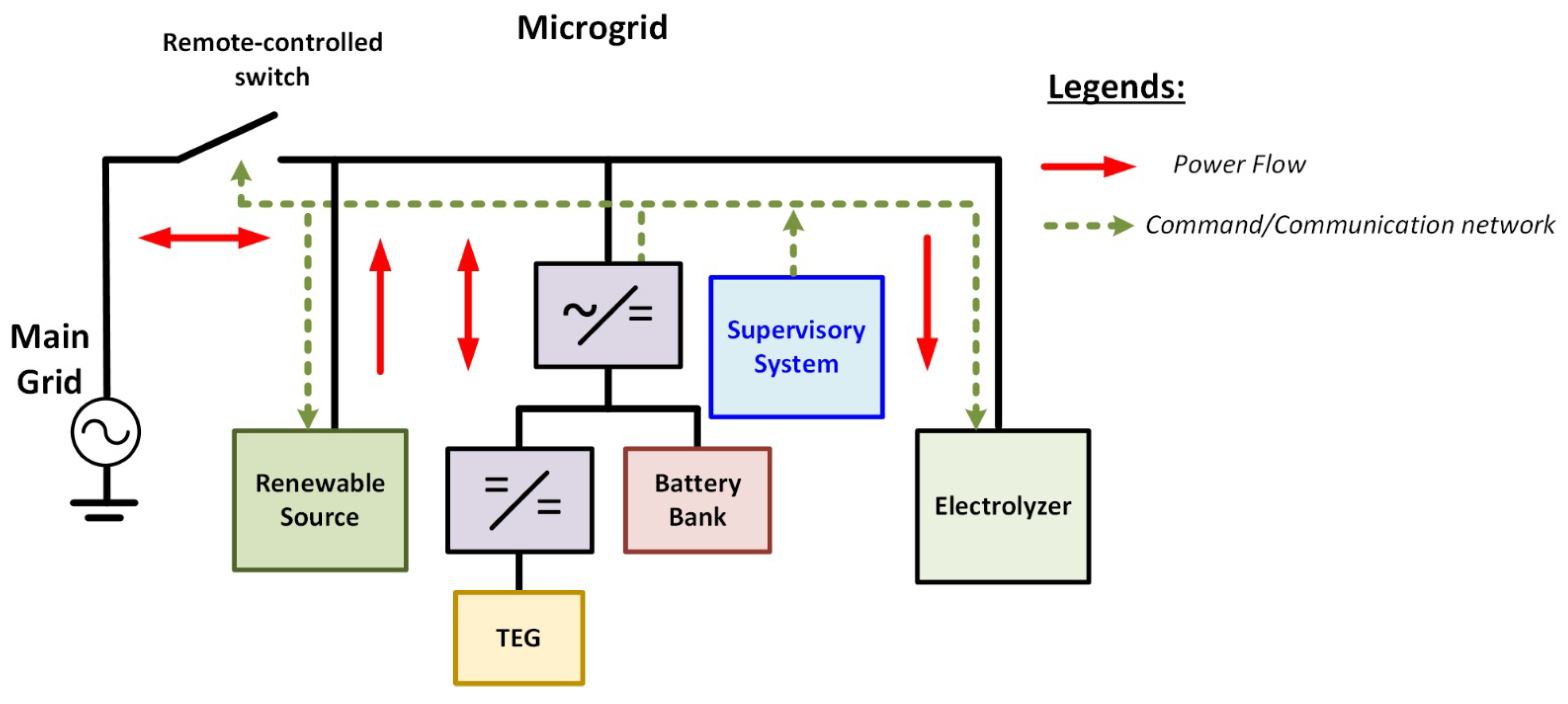
The 12 kW power laboratory comprises a combination of commercial components and in-house developed hardware and software prototypes. This configuration aims to create a straightforward yet resilient testing environment capable of emulating the intricate behavior and dynamics of a microgrid. The electrical setup follows a three-phase structure, with a 220 V line-to-line voltage operating at 60 Hz, aligning with the established standard for the Brazilian low-voltage grid.

Figure 1 presents the arrangement of all laboratory components. As depicted, alongside the generation sources, storage systems, and loads, the laboratory features a supervisory system. This system assumes responsibility for the synchronized monitoring and control of microgrid components.

Furthermore, the laboratory makes easier testing under islanded mode operation, where the microgrid is deliberately isolated from the primary grid through a remotely controlled switch. During this mode, the converter linked to the storage system and TEG cogeneration assumes the role of a grid-forming converter. It can not only identify instances of main grid disconnection but also effectuate reconnection once the primary grid is restored to operation.

2.1. PV System

To emulate PV generation, a commercial three-phase photovoltaic inverter, presented in Figure 2 and

Table 1. Basic characteristics of the Fronius Symo Brazil photovoltaic inverter [25].

Inverter	Fronius Symo Brazil
Numbers of MPPT	2
MPP voltage range	300–500 V
Total power	10 kW
AC output voltage	208–240 V

, was selected. Opting for this commercial inverter is guaranteed, given its pre-existing algorithms tailored for photovoltaic operation. Moreover, its nominal power and voltage align seamlessly with the microgrid’s designated parameters. The tri-phase capability enables uniform power injection across all three phases. Consequently, this singular inverter adeptly emulates, efficiently and cost-effectively, the impact of a PV farm integrated within the microgrid.

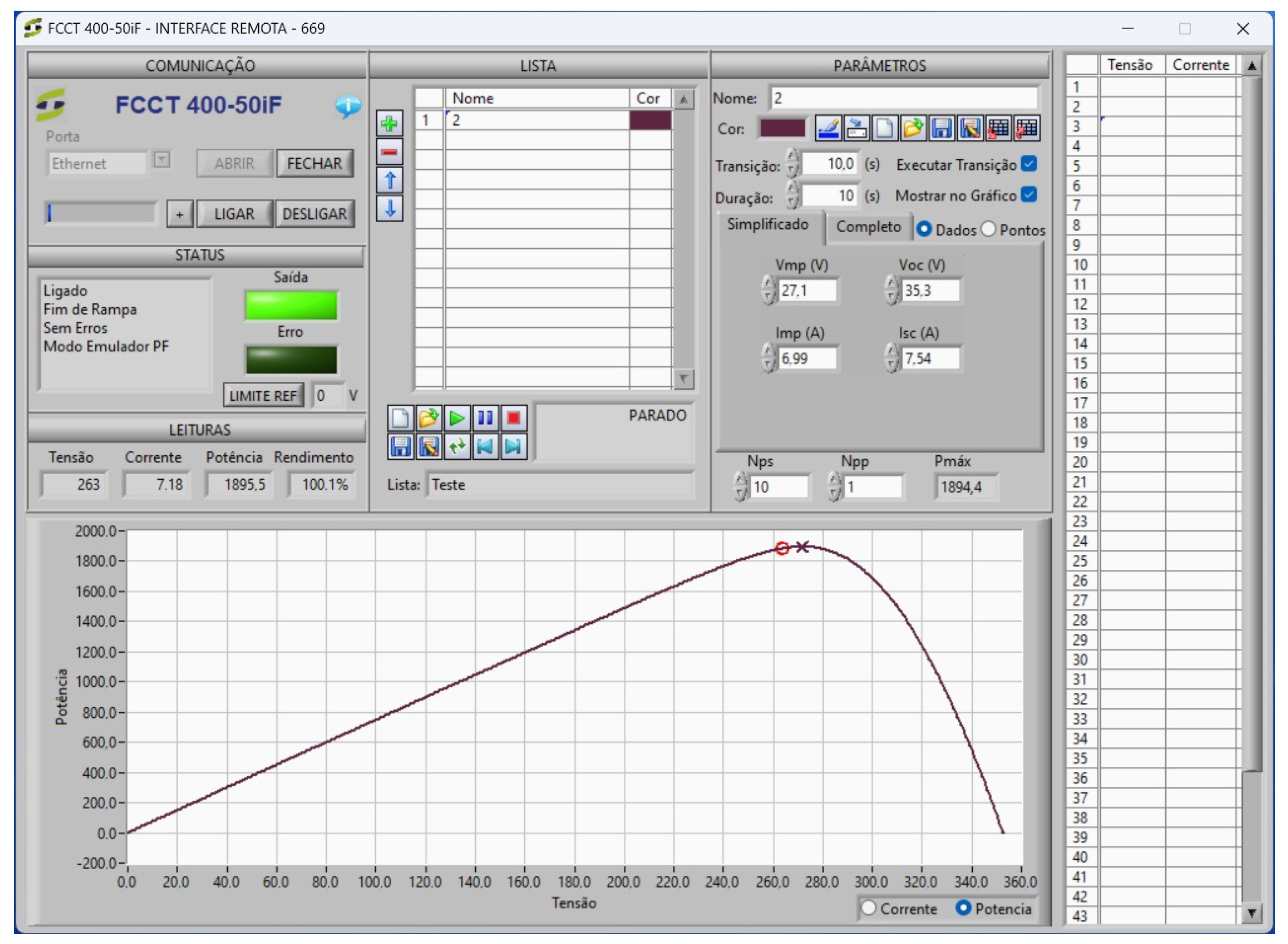
To circumvent reliance on solar irradiance, which is inherently intermittent, a deliberate choice was made to energize the inverter via a regulated voltage source capable of simulating the standard $PxV$ curve exhibited by PV panels. Employing this controlled voltage source offers the advantage of spatial optimization within the laboratory. This approach proves especially practical, as a photovoltaic panel array would necessitate a larger installation area. The structure of the controlled voltage source is shown in Figure 3 and

Table 2. Basic characteristics of the controlled voltage DC source [26].

Power supply	FCC 400-50i
Output voltage range	0–500 V
Output current	0–8 A
Output power	4 kW

.

To parameterize the PV curves utilized throughout the testing process, the voltage source manufacturer supplies software that empowers users to tailor the intended $PxV$ curve characteristics. This software additionally affords the flexibility to establish multiple $PxV$ curves concurrently, enabling adjustments to generation levels and maximum power points over regular intervals. Figure 4 illustrates the software’s parameterization interface. This interface allows for the definition of parameters linked to the PV configuration. For instance, users can specify the voltage of the PV panel, the quantity, and the arrangement within the array.

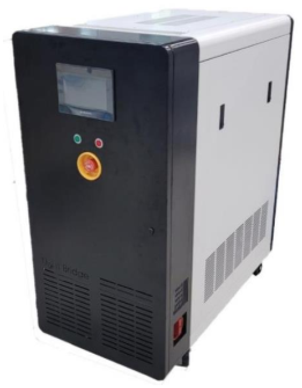
2.2. Electrolyzer

The laboratory is also equipped with a 5 kW alkaline electrolyzer, enabling the emulation of a microgrid incorporating a hydrogen production facility. The selection of an alkaline electrolyzer was based on its established maturity, commendable efficiency compared to other burgeoning water electrolysis technologies, and cost-effectiveness [27,28].

While the equipment is commercially available, its software has been customized to integrate control features and facilitate full external control. These added functionalities encompass the regulation of voltage and current during the electrolysis process. This enhancement empowers the system operator with greater autonomy over the operational processes.

When it comes to electrical infrastructure, it is necessary to use a transformer to adjust the 220 V of the laboratory grid to 380 V of the nominal input voltage of the inner controlled DC voltage source that feeds the equipment. The alkaline electrolyzer is shown in Figure 5 and

Table 3. Basic characteristics of the LBEX-5K Alkaline Electrolyzer [29].

Electrolyzer	LBEX-5K
Type of electrolysis	Alkaline
Power supply	220 V Three-phase
Power	<5 kW
Hydrogen production	1000 L/h
Oxygen production	500 L/h
Water consumption	800 mL/h
Hydrogen purity	99.7–99.9%
Oxygen purity	98%

.

2.3. TEG

Thermoelectric generators have been gaining substantial attention due to their noiseless operation, light weight, and compact design [30]. They have found successful applications in various fields, including solar energy harvesting, automobiles, biomedical devices, and industrial processes [31].

Indeed, TEGs have the remarkable capability to directly convert heat energy into electricity. This unique feature positions them as an ideal choice for capturing and utilizing waste heat produced in industrial processes. TEGs can operate efficiently even at extremely high temperatures, significantly boosting energy efficiency and aligning with eco-friendly practices in industries [32].

The Seebeck effect is the underlying idea behind TEGs. When there is a temperature difference, a voltage is created across two conductors connected in series and thermally in parallel [33]. This effect allows TEGs to harness energy that would normally be wasted as heat.

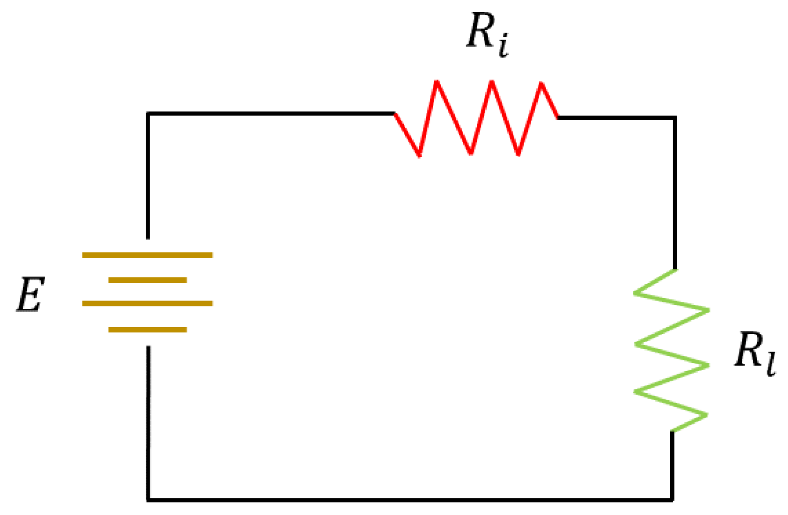
A thermoelectric generator module is normally made up of several interconnected legs that are placed on a common assembly base and coupled to ceramic sheets, essentially creating the hot and cold sides of the TEG module. The interfaces for the heat source and sink of the TEG module are located on the cold and hot sides, respectively.

A TEG can be thought of as the thermoelectric module’s equivalent electrical model [32]. The thermocouples used in the thermoelectric module are linked in series. A voltage source with internal resistance can serve as a representation for the electrically thermoelectric generator. Figure 6 shows an electrical schematic representing a TEG. The maximum power for the provided circuit is determined by the following Equation (1):

$$P=\frac{E^2}{4·R}$$

(1)

The maximum electrical output power from the TEG is achieved when the load resistance equals the equivalent internal resistance of the thermoelectric couples in series ($R_l=R_i$), resulting in each resistance receiving half of the source voltage [34,35].

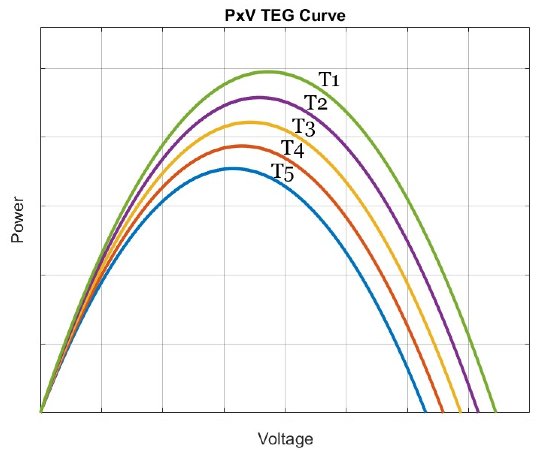
TEG modules, however, typically work in dynamic settings with stochastic temperature fluctuations. Because TEG output is a direct function of temperature, each module’s output power fluctuates under dynamic situations. Figure 7 shows a typically $PxV$ TEG curve. These curves vary according to the temperature gradient, which in the case presented is ($T_1>T_2>T_3>T_4>T_5$) and there is just one peak under each temperature gradient. Therefore, is essential to use an MPPT approach to maximize the power harvest of the TEG module by tracking the MPP.

To replicate the electrical model of the TEG devices depicted in Figure 6, we implemented the circuit as shown in Figure 8. This circuit incorporates a diode rectifier, powered by a variable autotransformer responsible for enabling voltage variation in the circuit, akin to the effect induced by temperature gradients. Additionally, a coupling transformer was employed to galvanically isolate the circuit from the AC network that powers it. The rectifier’s output includes a series resistor designed to simulate the internal resistance of the TEG device.

Table 4. Basic characteristics of the TEG system emulator circuit.

Internal DC voltage	0–560 V
Internal resistance	96 $\mathrm{\Omega }$
Maximum output power	830 W
Rectifier capacitance	5000 $\mathrm{\mu }$F

provides the parameters associated with the TEG system emulator circuit.

2.4. Battery Storage System and TEG Converter

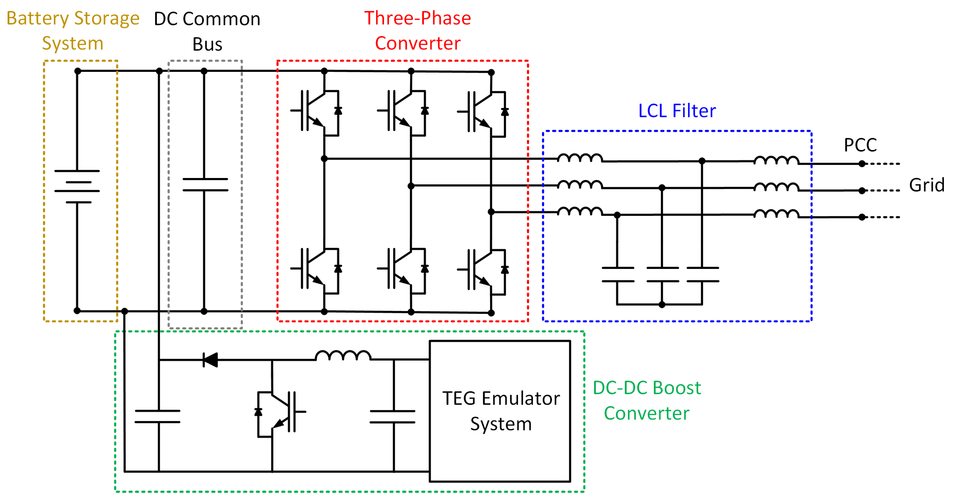
The integration of the battery storage system and TEG generation was strategically devised to streamline the laboratory’s infrastructure and leverage a common processing board for controlling both systems. This architecture consists of two converters that jointly utilize a shared DC bus, with the battery bank also linked to it. Figure 9 provides an illustrative schematic of the integrated system and its hardware layout.

The first converter is a three-phase AC-DC converter employed to establish the link between the DC bus and the grid. It assumes the roles of managing both battery bank charging and discharging and functioning as a grid-forming unit during islanded operations. The second converter is a boost DC-DC converter tasked with tracking the maximum power point of TEG systems and aligning the TEG voltage with the DC-link voltage. Importantly, it is worth noting that neither of these converters is commercial; both have been specifically developed and implemented to cater to the laboratory’s specific requirements.

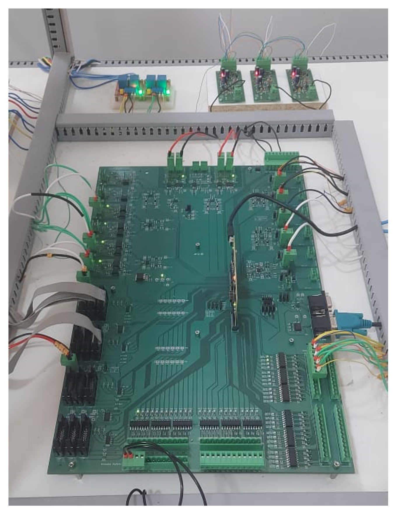
To develop control algorithms for the converters, the microcontroller TMS32028379D was employed. Its control card is connected to a motherboard (based on the design available in [36]), enabling access to the microcontroller pins pertinent to PWM modules, GPIO ports, serial communication, and signal conditioning for measurements. This circuit board, along with the associated peripherals and DSP control card, is illustrated in Figure 10.

The three-phase converter and the battery storage system were sized considering a nominal power of 6 kW, which is half the power of the laboratory capacity. This PWM-based converter incorporates an LCL low-pass filter designed to attenuate the impact of high-order switching frequencies. In developing the filter, the methodology explained in [37] was followed. The converter positioned on the laboratory workbench is shown in Figure 11 and

Table 5. Basic characteristics of the three-phase converter.

Rated power	6 kW
Current	16 A
Input voltage	486 $V_{cc}$
Output voltage	220 $V_{ac}$
Switching frequency	10,020 Hz
Inductance	1.3 mH
Inductance	790 $\mathrm{\mu }$H
Output capacitance	16.4 $\mathrm{\mu }$F

.

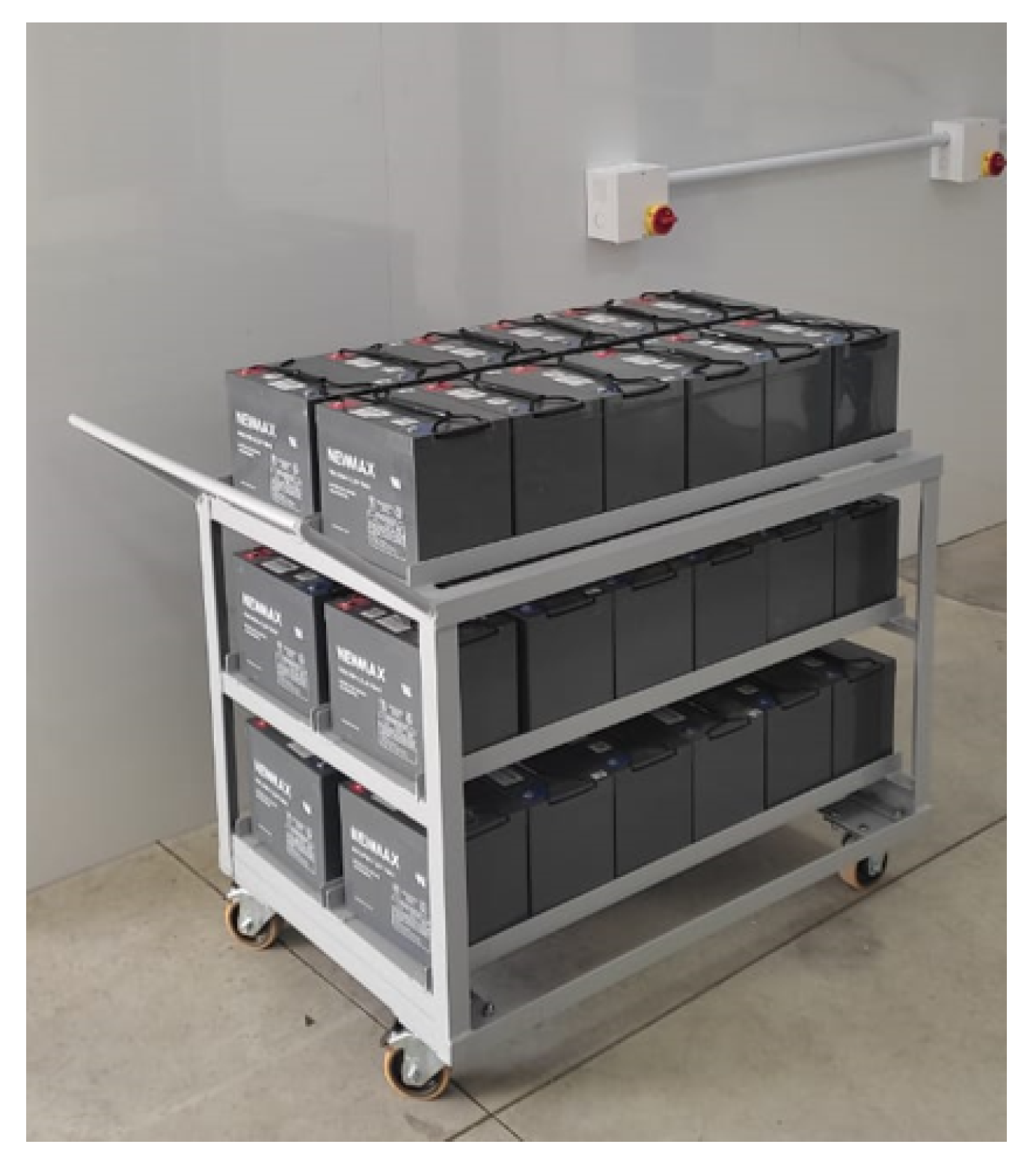
The battery bank is composed of 12 V sealed lead-acid batteries, each with a capacity of 70 Ah. Because this work deals with a prototype storage system by batteries with an interface made through a multilevel converter, factors such as weight and battery life were not a major concern. So, the selection of this battery technology is underpinned by its cost-effectiveness, user-friendly operational attributes, and inherent resilience in comparison to alternative battery technologies [38,39,40]. To ascertain the appropriate number of modules to constitute the battery bank, it is imperative to account for the AC voltage of the grid. This is crucial as power injection into the grid by the converter is feasible only when the DC link voltage, which is determined by the battery bank, exceeds the peak AC voltage.

The equation for determining the AC output voltage of the three-phase converter is represented by Equation (2). Here, $V_{dc}$ denotes the DC voltage, ma represents the modulation index that spans between 0 and 1, and $V_{f-f}$ signifies the RMS value of the line-to-line voltage of the converter. In this context, by adopting a modulation index of 0.95 and acknowledging the 220 V grid voltage, the threshold for the minimum acceptable DC link voltage stands at 378 V.

$$V_{f-f}=0.612·ma·V_{cc}$$

(2)

As the objective is to reach the minimum voltage level solely when the battery bank modules are fully discharged, the calculation for the number of modules involves dividing the minimum voltage by 10.5 V, which signifies the terminal voltage of an individual battery module. Consequently, to surmount the limitation imposed by the DC-link voltage, the battery bank needs to encompass 36 modules connected in series. The battery bank configuration is shown in Figure 12 and

Table 6. Basic characteristics of the battery bank.

Battery	FNC12700-C
Cells per monobloc	6
Rated voltage	12 V
Rated capacity	70 Ah
Max load current	28 A
Float charge voltage	13.5–13.8 V
Cyclic charge voltage	13.8–15 V
Discharge voltage	10.5 V

. Importantly, it is worth highlighting that this storage system can deliver a consistent 6kW power output, equivalent to the converter’s nominal power for approximately 5 h.

Given the low-voltage operational context of the TEG generation system emulation, a DC-DC boost converter was meticulously designed. Its purpose is twofold: firstly, to facilitate the injection of power from this system into the shared DC bus, where the battery bank is interfaced; secondly, the TEG devices generate power at a maximum power point, requiring the DC-DC converter to adeptly track this point.

Given that the nominal voltage of the shared DC bus mirrors the voltage of the battery bank, the boost converter’s output voltage must surpass 432 V. For design purposes, an output voltage of 500 V was adopted. Conversely, the input voltage hinges on the minimum voltage yielded by the TEG emulation system, which has been set at 50 V. With these voltage parameters established, and considering the TEG emulation system’s capacity as 500 W, the necessary inductor and capacitor for the DC-DC converter can be computed using Equations (3) and (4), respectively. Within these equations, $F_s$ symbolizes the switching frequency, ${\Delta }_{IL}$ signifies the desired input current ripple, and $\Delta V_{out}$ represents the desired output voltage ripple. The equations additionally take into account the duty cycle (D), which is evaluated using Equation (5). The DC-DC boost converter is installed on the laboratory bench as shown in Figure 13 and

Table 7. Basic characteristics of the DC-DC boost converter.

Power	800 W
Input voltage	150–280 V
Output voltage	486 V
Input current	3 A
Output current	1.65 A
Switching frequency	10,020 Hz
Input current ripple	1 A
Output voltage ripple	50 V
Inductance	5 mH
Output capacitance	18 μF

.

$$L=\frac{V_{in}D}{\Delta I_L{f}_s}$$

(3)

$$C=\frac{V_{out}D}{f_s\Delta V_{out}R}$$

(4)

$$V_{out}=\frac{V_{in}}{1-D}$$

(5)

3. Control

This section presents the control loops pertinent to the newly devised converters. The control loop for the three-phase converter encompasses the diverse operational modes exhibited by this equipment, encompassing battery charging and discharging, along with island mode operation. Furthermore, the section delves into the dead-time compensation algorithm, which plays a crucial role in mitigating harmonic components within the current waveform.

This section also addresses the control loop associated with the DC-DC boost converter that serves as the interface between the TEG generation system and the DC common bus. This converter must be able to extract the maximum power available from the generation devices. To achieve this, a P&O-type MPPT algorithm is utilized.

3.1. Discharge Mode

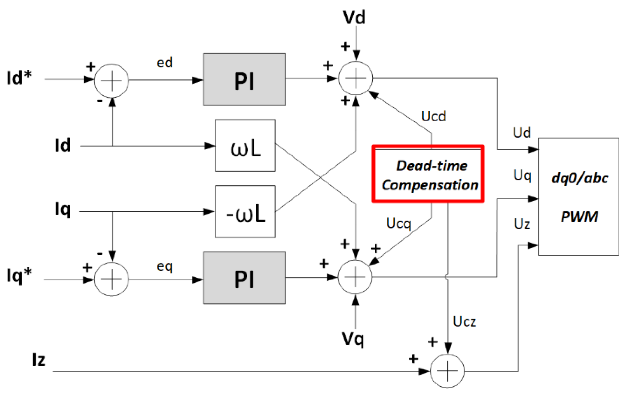
The converter’s discharge mode, involving power injection into the grid, is managed through a synchronous reference-based control strategy designed to effectuate decoupling between direct and quadrature axis parameters, as depicted in Figure 14. The reference angle employed for executing the synchronous transformation is derived from a phase-locked loop algorithm. This PLL algorithm is synchronized with the point of common coupling voltage.

The control architecture consists of two proportional-integral controllers, tasked with tracing the direct axis ($Id$) and quadrature ($Iq$) currents intended to flow between the converter and the grid. The direct current component ($Iq$) is directly tied to the active power managed by the converter, while the quadrature current component ($Iq$) pertains to the exchange of reactive power. The control framework further incorporates two decoupling terms, influenced by the network’s nominal frequency ($\omega$) and the converter’s filter inductances (L).

Moreover, the control loop incorporates a feedforward component in which the magnitudes of the grid voltage’s direct axis ($Vd$) and quadrature axis ($Vq$) are utilized. This feedforward element serves to counteract external fluctuations and enhance the control’s responsiveness and dynamics [41].

Since the converter’s objective is exclusively concerned with active power regulation, the quadrature current reference ($I{q}^{*}$) introduced by the converter into the grid is maintained at zero. The manipulation of active power exchanged with the grid is achieved by adjusting the magnitude of the direct axis current injected by the converter ($I{d}^{*}$).

To counteract the harmonic components arising from the driver dead time, a control loop founded on the non-ideal proportional resonant controller is employed, depicted in Figure 14 as a red block. These controllers take on the role of generating a voltage reference, which the converter utilizes to mitigate the presence of harmonic constituents within the output current.

The adoption of the non-ideal proportional resonant controller is substantiated by its diminished susceptibility to the precision of resonant frequency, as opposed to the ideal PR controller. The ideal PR controller exhibits an infinite gain at the resonant frequency, a characteristic that can potentially lead to stability concerns. In contrast, the non-ideal PR controller maintains a finite gain at the resonant frequency, albeit sufficiently high to curtail minor steady-state errors. Additionally, this design permits the expansion of the bandwidth in the proximity of the resonant frequency, thus decreasing sensitivity to minor frequency deviations [42].

Given the necessity to address multiple frequencies for compensation through the converter, the control loop is formulated by amalgamating multiple PR controllers into a singular controller. Within Equation (6), $K_p$ denotes the proportional gain, $k_r$ signifies the resonant gain, w represents the resonant frequency, and $w_c$ stands for the controller’s bandwidth. The index n designates the harmonic order corresponding to the transfer function.

$$G\left(s\right)=K_p+\sum _{i=1}^m\frac{2k_{ri}{\omega }_{ci}s}{s^2+2{\omega }_{ci}s+{\omega }_i^2}$$

(6)

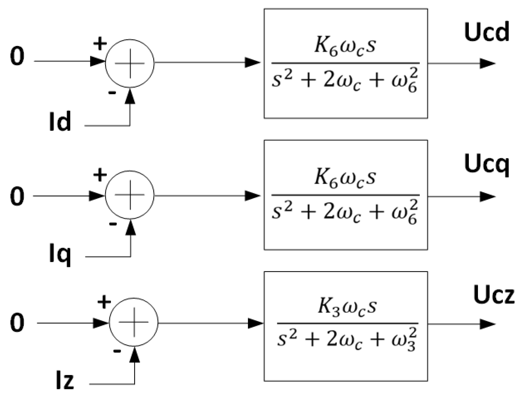
The prominent harmonic components stemming from the dead-time effect are principally the 180 Hz (3rd harmonic, $w3$), 300 Hz (5th harmonic, $w5$), and 420 Hz (7th harmonic, $w7$) frequencies. Because compensation takes place in the synchronous reference, the 5th and 7th harmonics manifest as a 360 Hz component (6th harmonic) within the $I_d$ and $I_q$ signals [43]. However, the 180 Hz current’s harmonic component is homopolar, remaining unaltered by the synchronous transformation and consequently appearing as a 180 Hz signal within the zero frame.

Consequently, a pair of non-ideal PR controllers tuned to 360 Hz are harnessed to counterbalance the fifth and seventh harmonics in the d and q frames. In parallel, another PR controller is engaged to offset the third harmonic in the zero frame. The control architecture of the dead-time compensation is depicted in Figure 15. It is noteworthy that the reference signal for the control loop remains at zero for all harmonics being addressed.

The control outputs derived from these controllers are combined with the primary controller signal in the $dq0$ frame, corresponding to the 60 Hz component. The resultant control signal is subsequently converted to the abc frame and modulated using the pulse width modulation technique. This modulation process generates the current waveform to be injected into or withdrawn from the grid by the equipment.

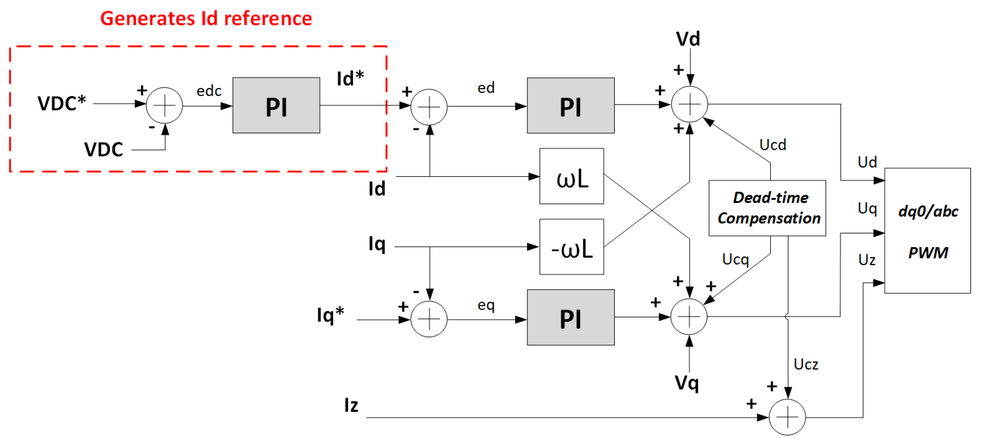
3.2. Charge Mode

The structure of the controller overseeing battery charging remains akin to the one elucidated in the preceding section, diverging solely in the methodology employed for generating the reference component $Id$ to be followed by the converter. The generation of the direct axis current reference ($I{d}^{*}$) hinges on the operational stage in which the charging process currently resides. These stages are categorized as constant current, constant voltage, and floating mode [45,46].

Figure 16 delineates the progression through the three operational stages of the lead-acid battery. Notably, in stage 1, characterized as the constant current mode, a steady DC current is set to charge the batteries. Throughout this stage, the voltage rises linearly until it reaches the floating voltage threshold. In the constant current mode, a proportional-integral controller is employed to trace the DC current reference ($ID{C}^{*}$). This PI controller generates the current reference ($I{d}^{*}$) to be pursued by the controller, as shown in Figure 17. The charge current value is predefined by the user during device initialization.

The transition into stage 2, recognized as the constant voltage mode, commences upon reaching the floating voltage level. In this phase, the DC current commences a gradual decay over time to maintain the battery at its floating voltage. To accomplish this, a proportional-integral controller dedicated to tracking the battery’s floating voltage takes charge. This PI controller generates the current reference $Id$ to be followed by the controller, as shown in Figure 18.

Lastly, stage 3, recognized as the fluctuation stage, essentially extends from stage 2. During this phase, a minor charge current is drawn from the grid solely to maintain the battery’s voltage in a fluctuating state. Consequently, the control loop employed for this operational stage remains identical to that utilized in stage 2.

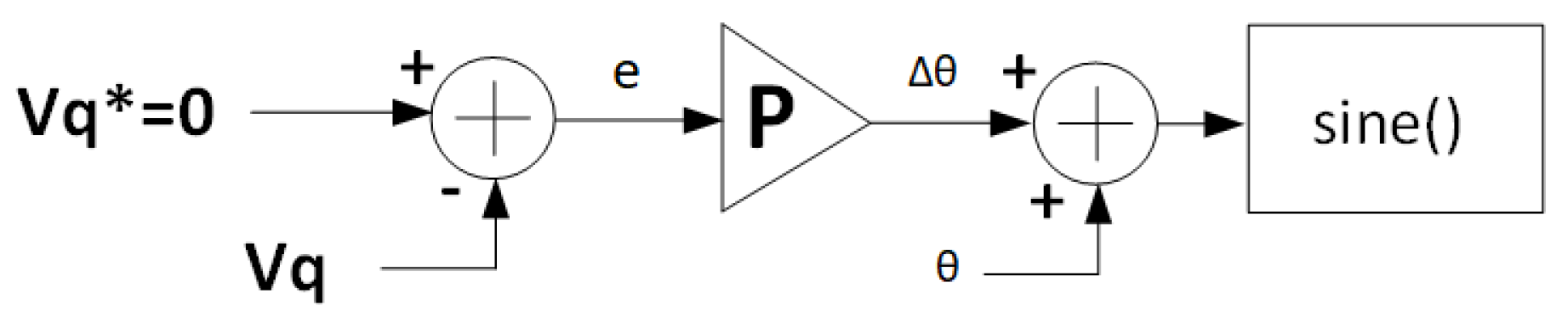
3.3. Island Mode

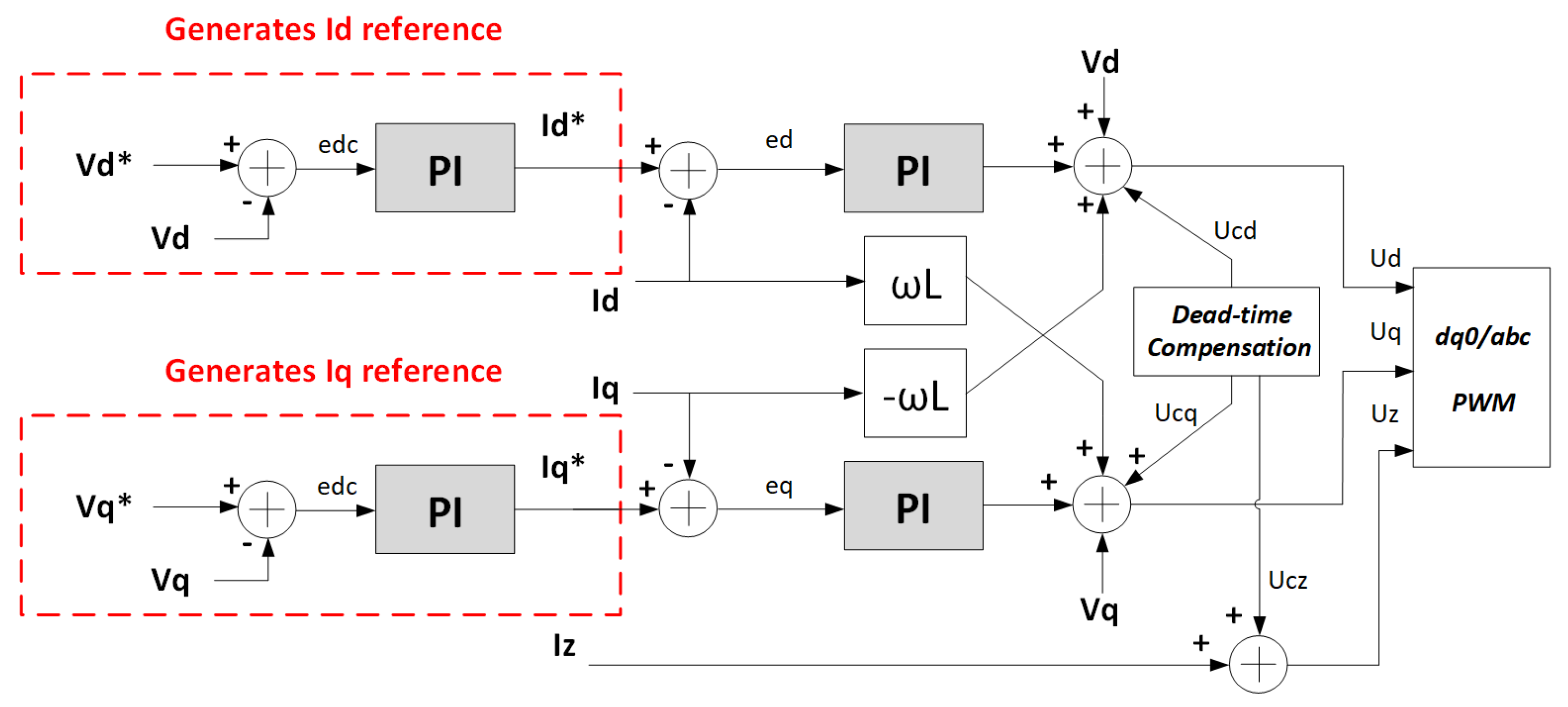
The island mode control employs the identical inner $dq0$ current control loop that has been elucidated in other operational modes, as expounded upon in preceding sections. However, what distinguishes the island mode control is the exterior control loop, responsible for generating the $dq$ current reference intended for the converter’s tracking. Given that the converter functions as a grid-forming entity, its role extends to generating a voltage reference for other equipment incorporated within the microgrid. This entails preserving both the voltage magnitude of the bus and its frequency at nominal values, regardless of the power output by the converter [47].

Consequently, in pursuit of this objective, a pair of PI controllers is deployed to track the $dq$ voltage reference. The outcome of this endeavor generates the direct and quadrature current references, as demonstrated in Figure 19. It is important to note that, in this context, the $Vd$ reference is established at the nominal phase-to-neutral voltage peak, while the $Vq$ reference is maintained at zero. In the context of island mode operation, the absence of an external voltage reference for control synchronization requires the creation of an internal 60 Hz signal. This signal is generated by the microcontroller to make easier operations associated with the $dq0$ transformation intrinsic to voltage and current control loops.

The adoption of this isochronous control strategy stems from the unique nature of the converter developed, which functions as the sole grid former within the microgrid. In a contrasting scenario where multiple grid-forming converters coexist within the grid, a droop control approach would be employed to orchestrate power distribution among them [48,49].

To detect the occurrence of a main grid loss, a passive method of islanding identification is harnessed. This method hinges on monitoring the direct voltage amplitude and tracking variations in frequency. Should either the voltage amplitude or grid frequency exceed predetermined threshold values, a command signal is transmitted to the remote-controlled switch. The frequency was chosen as a 1Hz variation from the network frequency. The voltage value chosen was a 10% variation from the phase-neutral voltage. This command disconnects the microgrid from the main grid, thereby isolating it in reaction to a detected main grid loss.

Passive methods of islanding identification exhibit a relatively lower immunity to non-detection zones when juxtaposed with active and hybrid methodologies. Nonetheless, despite this limitation, the passive approach was selected as the initial point of departure for islanding identification studies to be conducted within the laboratory facility. This choice is underpinned by the method’s inherent simplicity and cost-effectiveness, rendering it a pragmatic starting point for investigation [50].

Upon readiness of the main grid for reintegration, the grid-forming converter assumes the task of realigning the microgrid voltage with the main grid voltage before effectuating their reconnection via the closure of the remote switch. This procedural step is critical to circumvent any abrupt power transients between the two systems during reconnection, which might otherwise jeopardize the integrity of the microgrid equipment. As such, the employment of a resynchronization algorithm emerges as a paramount consideration in this process.

The implemented algorithm takes on the role of phase angle adjustment within the internally generated sine wave, which serves as the converter’s reference during island mode operation. This alignment is pursued until the reference sine wave attains synchronization with the main grid voltage, thereby enabling the reconnection process. This synchronization endeavor is accomplished through the application of a proportional gain. Upon restoration of the main grid’s operation, the algorithm works to mitigate the quadrature voltage component ($Vq$) of the main grid. Given that, during island mode operation, $Vq$ is derived from the converter’s tracking of the reference sine wave, its value is intrinsically linked to the phase discrepancy between the voltages of the two systems.

As a result, the deviation between the $Vq$ value and the desired zero reference is employed to calculate an angle value ($\Delta \theta$) by multiplying it with the proportional gain. This calculated angle is subsequently added to the reference sine signal angle ($\theta$). Figure 20 illustrates the resynchronization algorithm, with the proportional gain (P) being configured at a suitably low level to ensure a gradual convergence. This approach safeguards against abrupt phase shifts during the process. Upon completion of this phase, the phase-locked loop algorithm begins utilizing the main grid voltage as its reference, thus paving the way for reconnection to occur.

3.4. DC-DC Converter Control

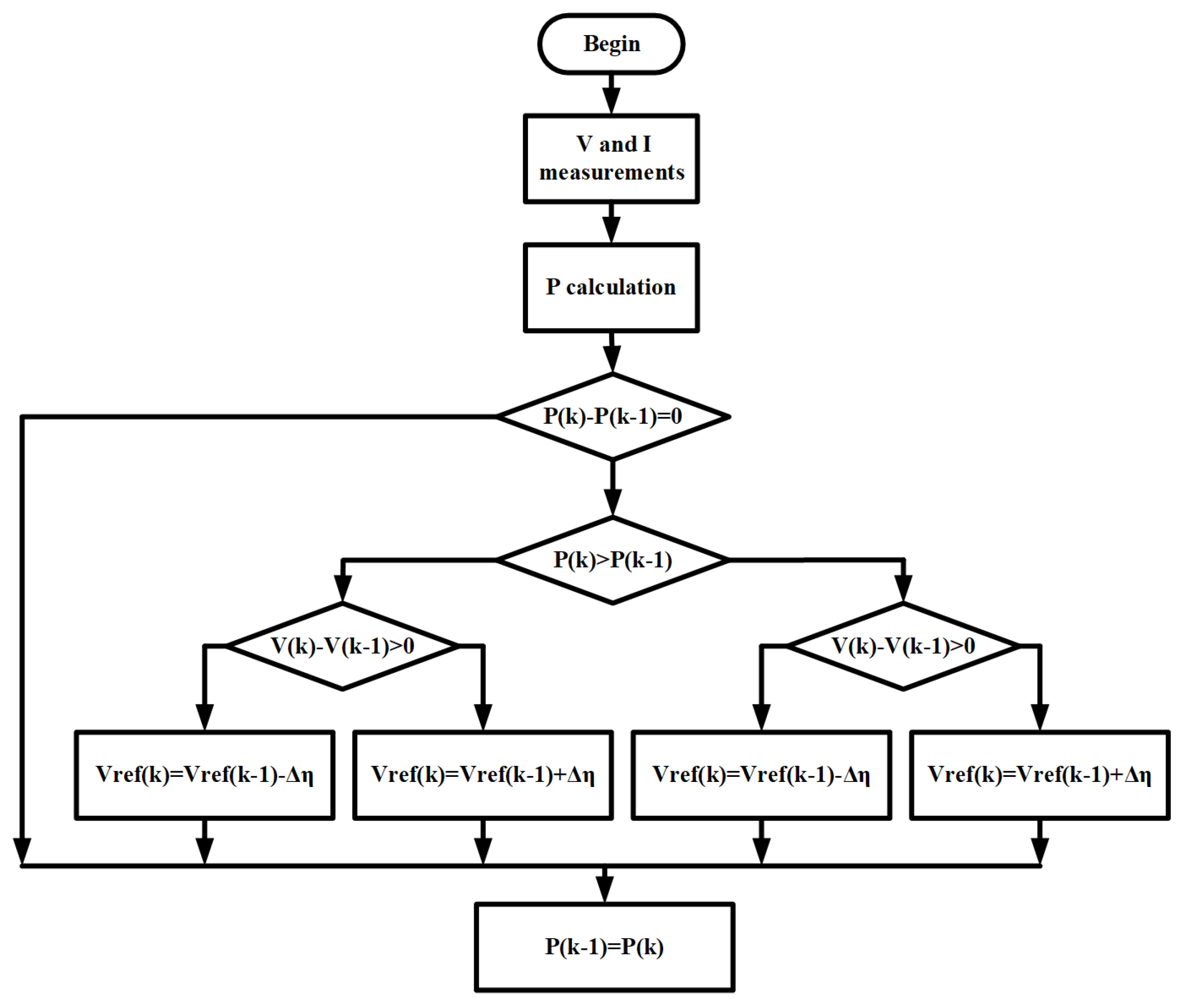
As previously detailed in preceding sections, the operational behavior of thermal generation can be simulated using a DC voltage source combined with a series resistance. This DC voltage source replicates the temperature gradient observed in TEG devices. Consequently, alterations in voltage levels lead to shifts in the operational point where maximum power extraction occurs. To effectively follow this maximum power point, it is essential to employ algorithms that can adjust to variations in thermal gradients. These algorithms are referred to as maximum power point tracking algorithms.

The perturb and observe technique entails introducing a minor perturbation to the operating voltage of the TEG system by adjusting the duty cycle of the DC-DC converter. Subsequently, the output voltage and current of the TEG system are measured, enabling the calculation of power, which is then compared against the power value preceding the perturbation. If the power increases, the algorithm proceeds with a perturbation in the same direction as the prior one and reiterates the power comparison process. Conversely, if the power at the new operating point diminishes, the voltage perturbation is executed in the opposite direction. Through this iterative process, the converter methodically traverses the entire power-to-voltage curve of the TEG device, progressively nearing the maximum power point. The operational sequence of the P&O algorithm is outlined in Figure 21. Here, the index k signifies the ongoing iteration, while $\Delta \eta$ denotes the voltage perturbation.

3.5. Communication Infrastructure and Supervisory System

To oversee all the constituents comprising the microgrid and facilitate remote control commands, the supervisory platform “Elipse E3” by Elipse is employed. This software encompasses a comprehensive array of functionalities essential for this project, encompassing:

• An open and friendly programming interface, based on the Visual Basic language;
• A wide range of drivers for communication with the most diverse devices;
• Speed of processing and communication;
• MS SQL Server database connectivity.

In addition to its device interface capabilities, the supervisory platform also dispatches operational set points to guide the behavior of these devices. For instance, it communicates directives like the desired current magnitude to be injected by the battery storage system into the grid or the specified current level for the electrolysis process. Furthermore, the supervisory platform governs the operational states of select equipment. A case in point is the battery storage system, which can be directed to function in charge, discharge, or idle mode as dictated by the supervisory commands. This overarching control enables precise management and coordination of the microgrid’s operations.

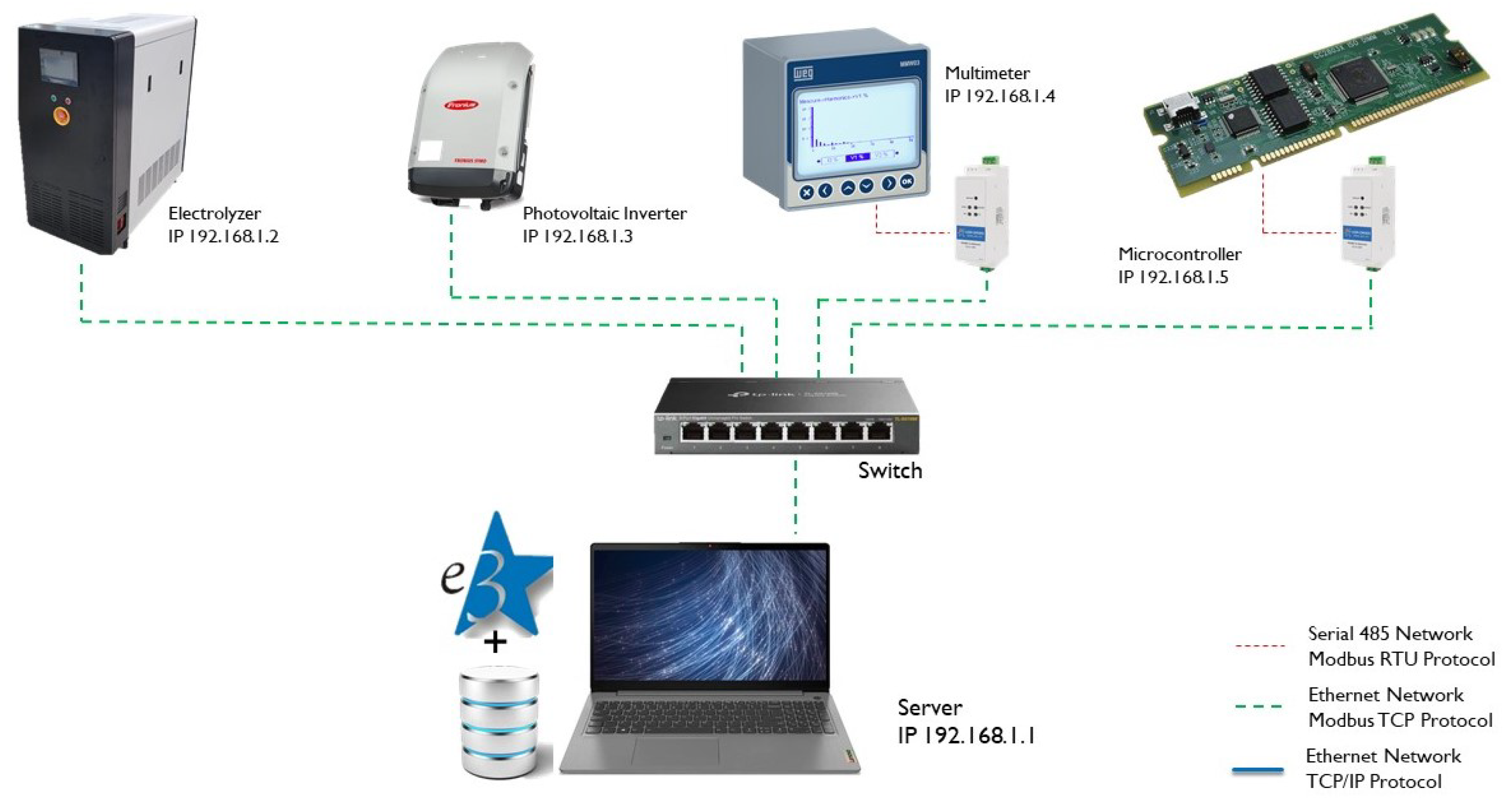
To facilitate communication with the grid components, the ModBus/TCP protocol has been adopted. This protocol’s selection stems from its blend of structural simplicity and widespread acceptance across diverse manufacturers. The network topology has been implemented as depicted in Figure 22, effectively reflecting the arrangement and connectivity of the grid components.

The electrolyzer and photovoltaic inverter devices inherently supported Modbus/TCP communication, necessitating only the configuration of IP addresses. However, the multimeter, entrusted with electrical measurements at the coupling point between the microgrid and the main grid, and the DSP microcontroller, responsible for the management of the battery bank and TEG converters, employed Modbus/RTU via RS485 and RS232 interfaces, respectively. Consequently, these devices necessitated a gateway to effectuate protocol conversion and interface adaptation, enabling their alignment with the Modbus/TCP standard.

The selection of the MS SQL Server database stems from its robustness, swift management capabilities, and notably, the potential for scalability in terms of database storage. This database is tasked with storing all the relevant parameters from each device, with a sampling frequency of 1 s per recording. Notably, all available variables within each device are meticulously monitored, affording programming flexibility and enabling the execution of studies on coordination solutions among microgrid agents and energy management strategies. The implemented SQL system has the following configurations: Windows 10, i7 8th generation, and 8 GB memory ram.

The supervisory platform additionally incorporates real-time trend graphs and historical data, offering a comprehensive overview of the primary information for each device. This empowers users with enhanced analytical capabilities. Moreover, the platform integrates an alarm mechanism that provides visibility into device failures and events. These alarms are presented to the user on-screen and simultaneously recorded in the database as reports, ensuring that operational insights are readily accessible.

4. Results and Discussion

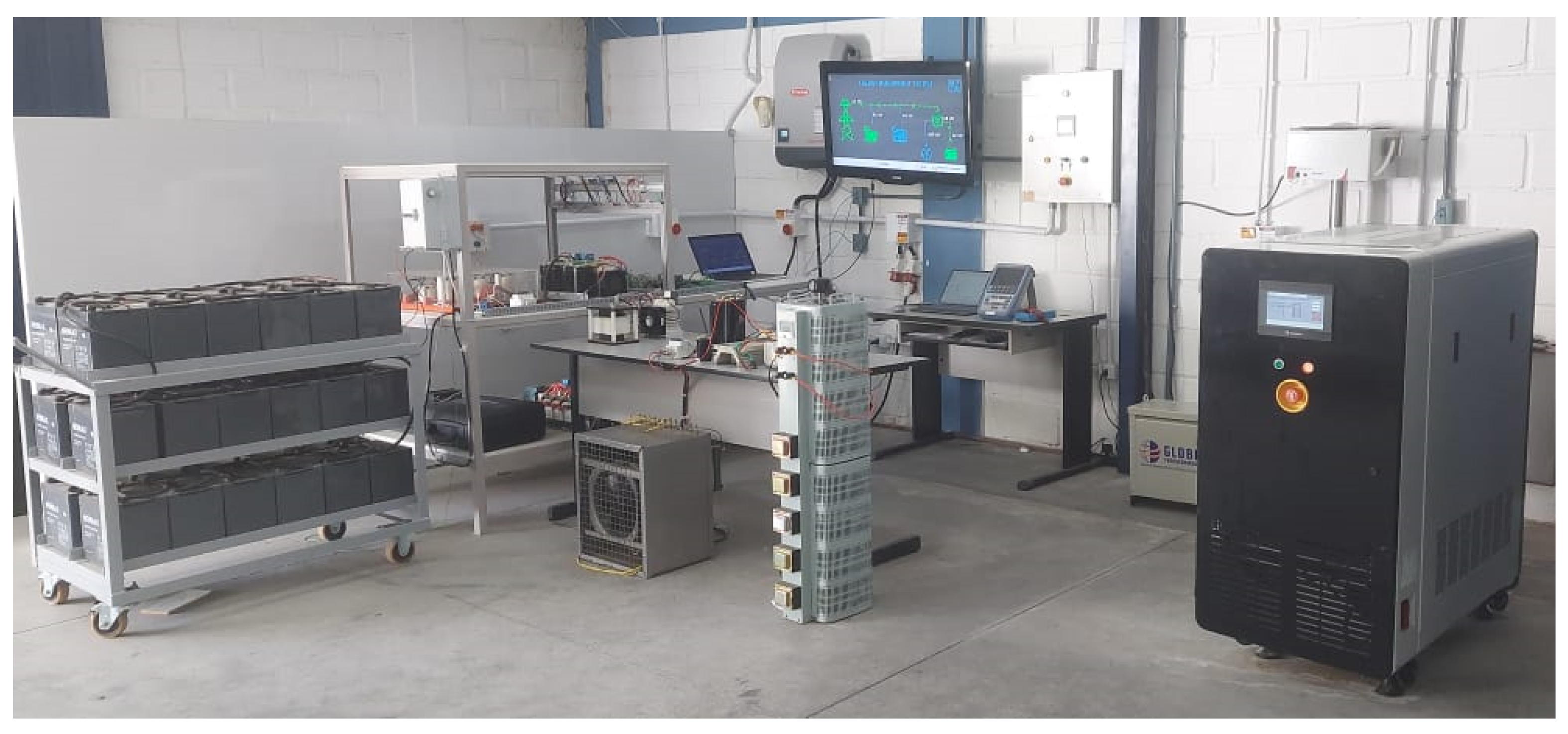
In this section, the results associated with the operation of the laboratory described in the previous sections are presented. Figure 23 depicts the final layout of the developed laboratory. While the overall operation of the laboratory is discussed, special attention will be given to the non-commercial devices that were developed during the project to meet the laboratory’s specific needs. These are as follows:

• A battery bank converter and network former;
• A converter associated with the simulated;
• A supervisory system.

4.1. Battery and TEG System

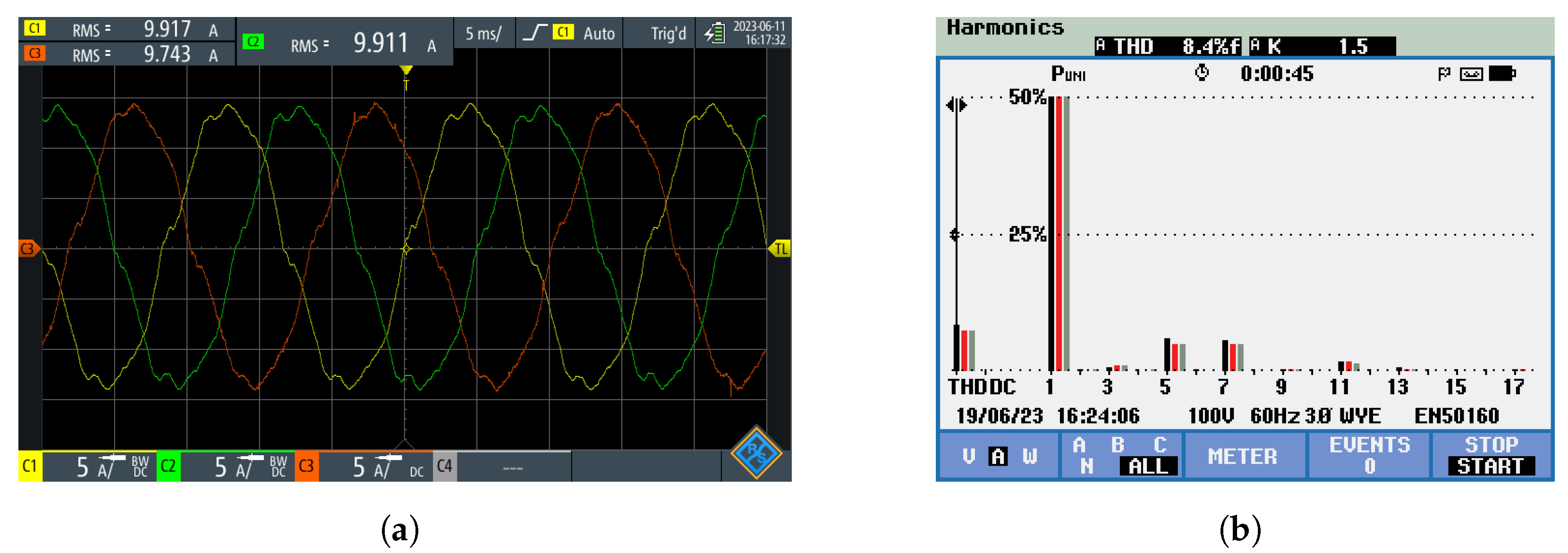
This subsection encompasses the outcomes linked to the performance of the three-phase converter and its controllers. In Figure 24a, the oscillograms illustrating the three-phase currents injected by the inverter are depicted, characterized by a reference of 10 A RMS and the absence of dead-time compensation. Complementary to this, Figure 24b elucidates the harmonic spectrum of these currents. Notably, it becomes evident that in the absence of compensation for the fifth and seventh harmonics attributed to dead-time effects, despite the controller’s capability to track the 60 Hz component, a significant harmonic content of the 300 Hz and 420 Hz constituents persists. This culminates in a total harmonic distortion of 8.4%.

Figure 25a encompasses both the oscillograph (a) and the harmonic spectrum (b) of the currents injected by the converter under analogous conditions as in Figure 24. However, in this instance, the compensation for harmonic components engendered by the dead-time effect is enabled. A discernible trend emerges in Figure 25b, illustrating the substantial reduction in the 300 Hz and 420 Hz components through this compensation process. The outcome is a pronounced decrease in the total harmonic distortion (THD), culminating in an acceptable value of 2.4%. Moreover, this compensation endeavor contributes to the enhancement of current waveform profiles.

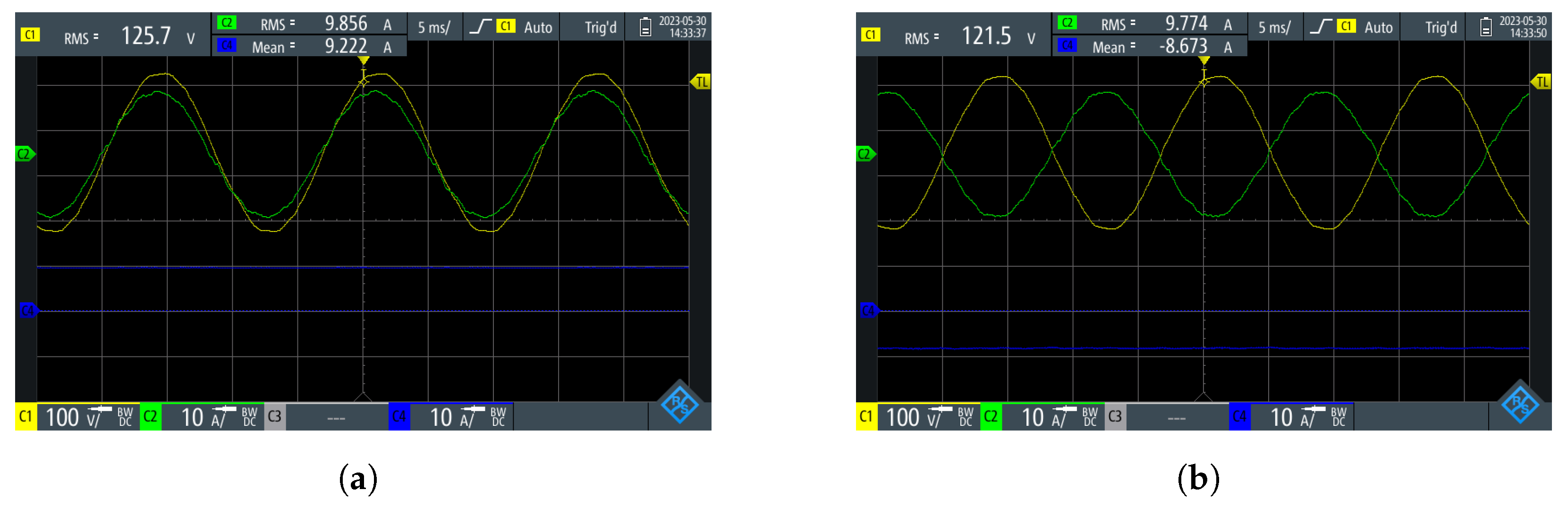
In Figure 26, the converter’s dual role of absorbing and injecting 10 A RMS into the network is illustrated. In Figure 26a, highlighting the injection mode, the current (illustrated by the green signal) is in phase with the neutral phase voltage (denoted by the yellow signal). This alignment leads to a discharge of DC current (indicated by the blue signal) from the batteries, averaging around 9 A. Conversely, in the absorption mode showcased in Figure 26b, the AC current operates in anti-phase relative to the grid voltage. Consequently, the DC current assumes a negative sign, signifying a reversal in the power flow direction.

The transient responses of the control for various current references are showcased. Figure 27a portrays an instance where the converter, initially operating by injecting a current of 5 A RMS (depicted by the green signal) into the AC bus to which it is linked, undergoes a reference alteration to 9 A RMS. Analyzing the behavior of the discharged DC current (represented by the blue signal) from the batteries, it can be deduced that the control attains stability with the new reference in approximately two cycles of 60 Hz.

Figure 27b exemplifies a scenario where the converter starts operation by injecting a 5 A RMS current into the AC bus. Subsequently, it shifts to absorbing a current of 9 A RMS within a span of nine cycles of 60 Hz. The prolonged adjustment duration observed here can be attributed to the extended interval between the first and second current references, which the controller endeavors to track.

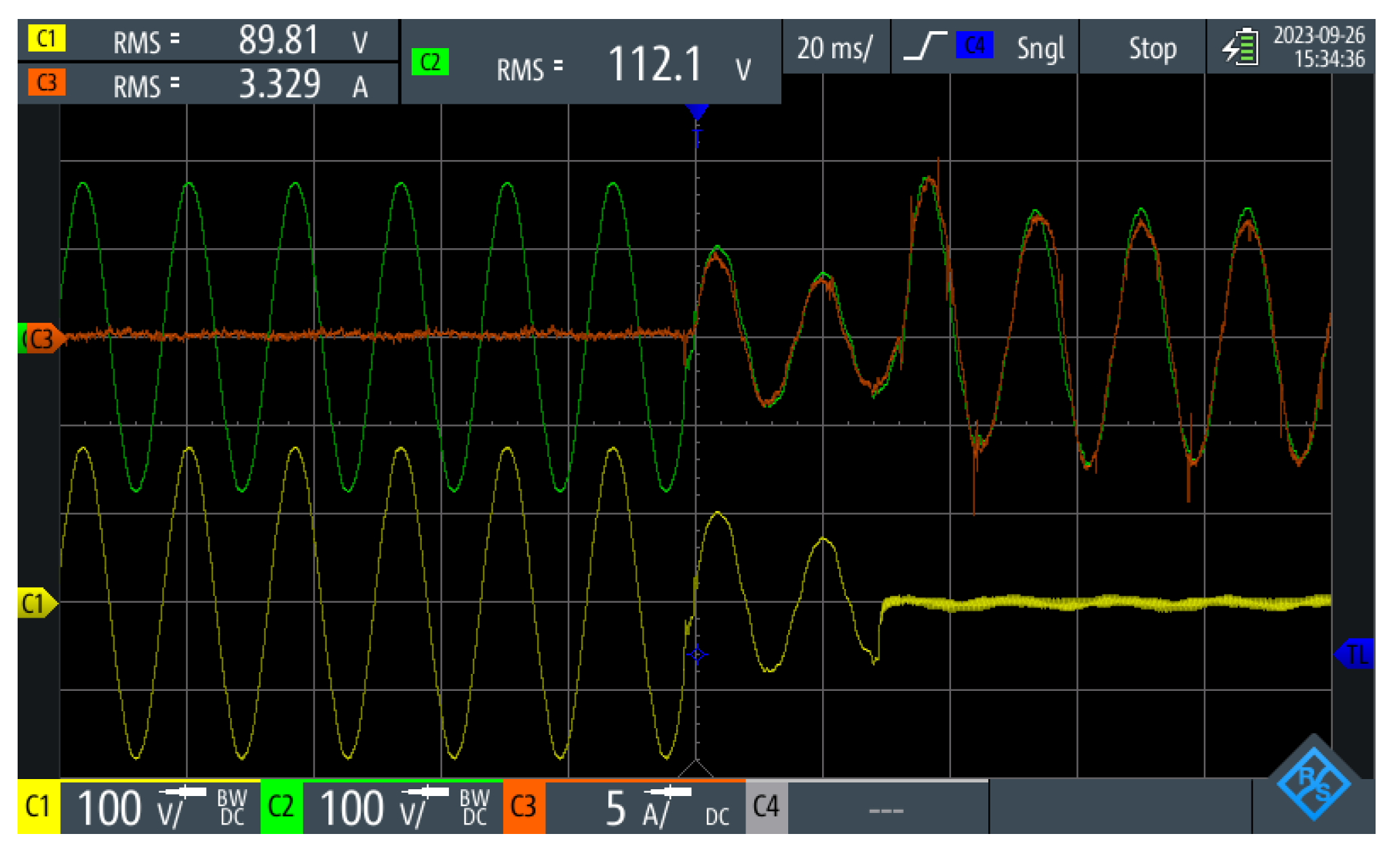
Figure 28 illustrates the operation of the boost converter during the MPP of the TEG-emulating system while undergoing a voltage variation. Initially, the internal voltage of the circuit (yellow signal) used to emulate the TEG system is 300 V. According to the theory described in previous chapters, the MPP occurs when the voltage at its terminals (green signal) is 150 V. As observed, at this operating point, the converter can reach the MPP, drawing approximately 2 A (red signal), resulting in an extraction of about 300 W.

After a few moments, the internal voltage of the circuit is raised to 500 V to emulate the increase in the thermal gradient of a set of TEG devices, and consequently, the increase in generated power. During this variation, the maximum power point shifts, prompting the boost converter, through the MPPT algorithm, to start tracking this new point. According to theory, this new point should be around 250 V, and as can be observed, the converter adjusts the system to this value in about 15 s. At this point, the extracted power from the circuit emulating the TEG set is 750 W.

The oscillations present in the voltage are primarily due to the duty cycle update step, where a $\Delta \eta$ of 0.003 was used. Reducing these oscillations can be achieved by using smaller steps. However, it prolongs the time required to reach the MPP. Operating points that require a higher duty cycle may also exhibit more oscillations. This is because the variation in converter gain is more sensitive to changes in the duty cycle at points where the latter is higher.

In general, considering the parameters of the circuit emulating the TEG system along with the theory of maximum power transfer, it was observed that the implemented boost converter was able to satisfactorily track the maximum power point of this system. Therefore, the hardware related to the boost converter and the system emulating the TEG system can be used in the future as a platform for the development and improvement of MPPT algorithms.

4.2. Charge Battery Bank Mode

This subsection delves into the battery bank’s charging cycle, wherein a DC current reference of 7 A was stipulated for the constant current mode, accompanied by a voltage reference of 468 V for the constant voltage mode. Figure 29 encapsulates the battery charge cycle executed over approximately 9 h.

Initially, the battery bank possessed an initial voltage of 424 V at the commencement of the charging process. Notably, the initial 4 h period encompasses the constant current mode, during which the battery absorbs the specified 7 A reference current. Over this stage, the voltage exhibits linear growth, ultimately attaining the predetermined 468 V threshold.

After this point, the control mechanism transitions to the constant voltage mode. In this phase, the current responsible for charging the bank progressively decreases to uphold the reference voltage. A noteworthy observation is the gradual reduction of the current drawn by the batteries as the charging cycle unfolds. Given the extended duration and the gradual tapering of current toward zero in stage 3, this phase has been omitted in the figure to preserve resolution in depicting the latter two stages.

In the final stage, only a residual current remains, serving to sustain the battery voltage at its designated float value. This culminates in the completion of the cycle and the cessation of battery charging.

4.3. Island Mode

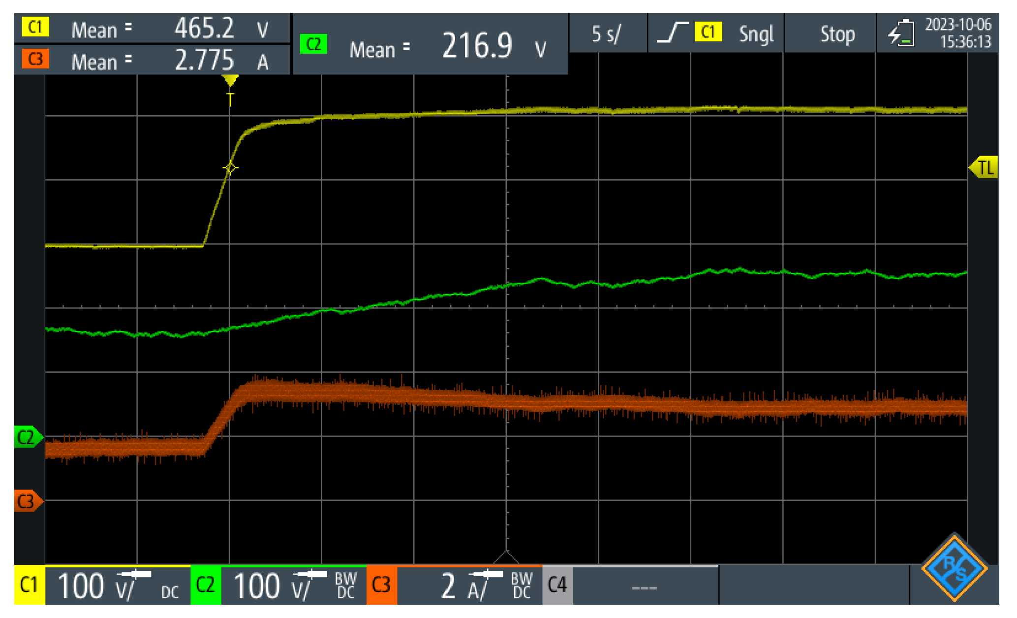
To demonstrate the effectiveness of the algorithms associated with microgrid islanding, we initially considered a scenario where the electrolyzer (load) consumes approximately 2kW of power, which is provided by the main grid. The converter connected to the battery bank, which operates as a grid former during islanding, is in a floating mode, meaning it does not exchange power between the bank and the grid. When a loss of the main grid occurs and is detected by the converter, a signal is sent to the switch that connects the microgrid to the main grid, and the disconnection is carried out. From the moment of disconnection, the grid-forming converter takes over, supplying the power demanded by the load while maintaining the nominal bus voltage.

The dynamics of the described procedure can be observed in Figure 30. Here, it is evident that the voltage of the microgrid (depicted in green) and the main grid (depicted in yellow) are initially equal, as both systems are connected. As previously mentioned, initially, the converter is in a floating state, which is indicated by the output current of the converter (depicted in red) being approximately zero.

When the main grid goes down, the converter takes two cycles to execute the disconnection and assume control of the bus. In this way, the converter starts maintaining the nominal voltage of the microgrid while also supplying the current required by the load.

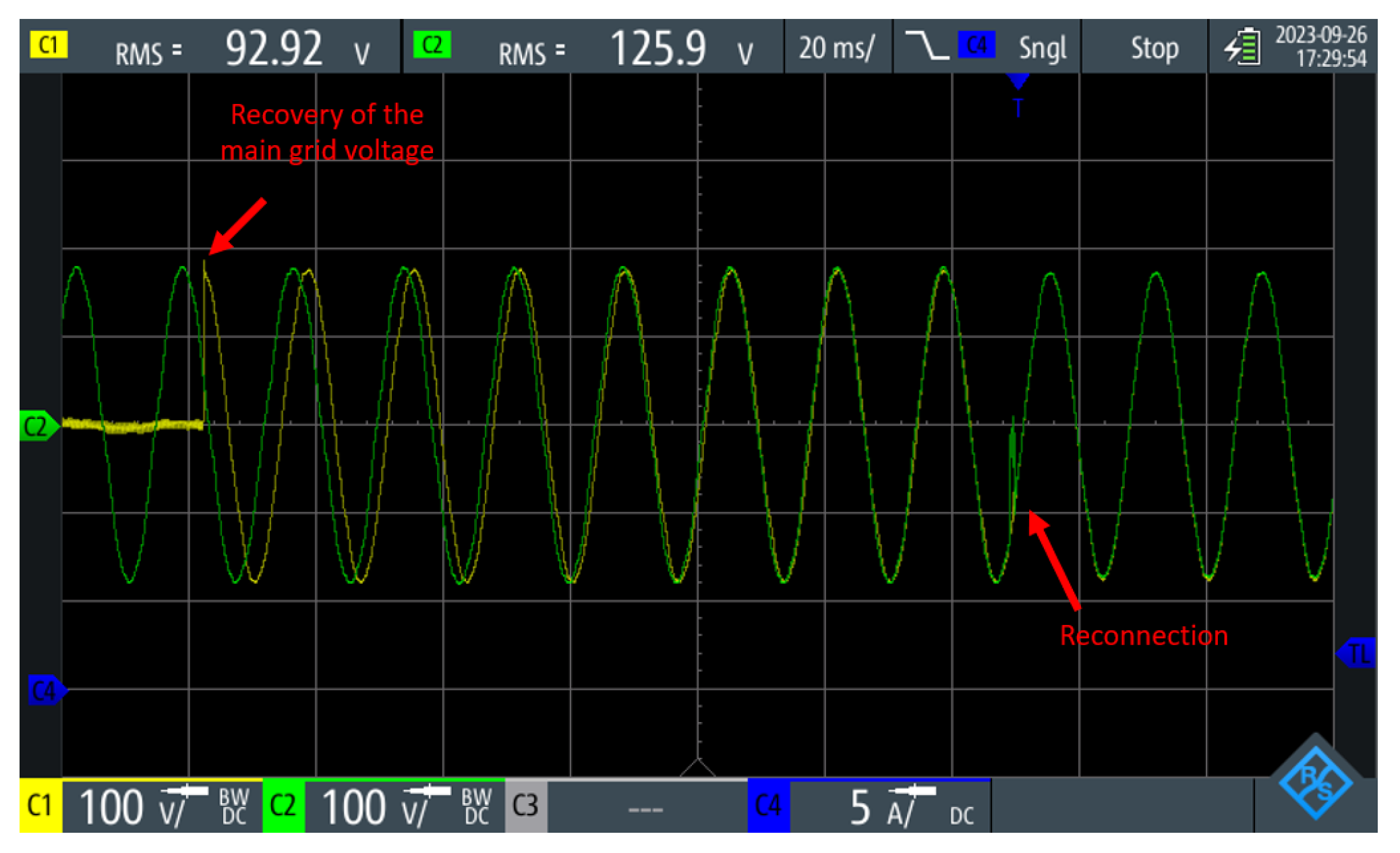
Upon the restoration of the main grid, the converter initiates the synchronization between the microgrid voltage and the main grid voltage. Consequently, once synchronization is achieved, a command is dispatched to the coupling switch, and reconnection is executed. The Figure 31 shows the dynamics of the synchronization between the main branch voltage (depicted in yellow) and the microgrid voltage (depicted in green). Here, it is observable that when the main grid is restored, its voltage is not synchronized with the microgrid voltage. Therefore, a slow resynchronization is necessary to prevent a sudden phase jump that could impact the load. When the phase difference between the voltages is sufficiently small, reconnection occurs. In this scenario, the reconnection process lasted approximately 7.5 cycles of the grid voltage.

4.4. Supervisory System

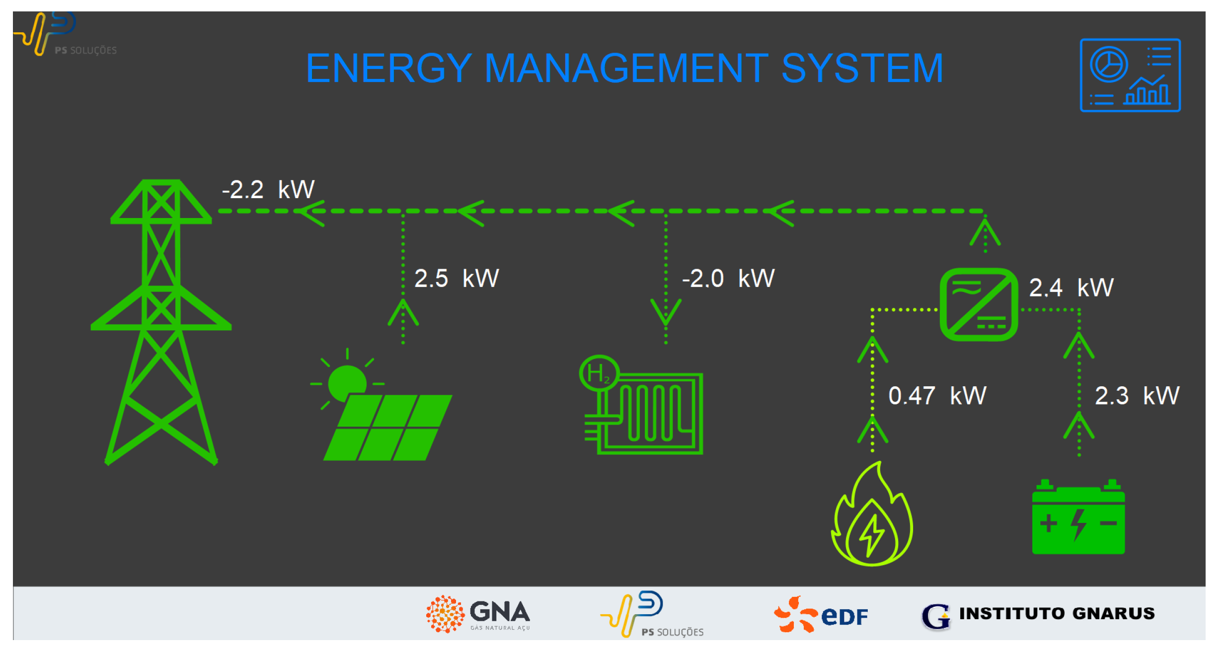
The main screen of the supervisory system is shown in Figure 32. It displays the status of all agents that make up the microgrid (whether they are connected or disconnected), represented by the icons. Additionally, the figure shows the power contribution of each of the devices connected to the microgrid, with arrows indicating the direction of power flow. In the presented case, all agents are connected and therefore displayed in green. If they were disconnected, they would be represented in blue.

In this scenario, there is cogeneration by the system emulating the TEG system (about 0.47 kW), and the batteries are being discharged into the bus, totaling 2.4 kW injected into the grid by the inverter that interfaces these systems with the grid. Additionally, there is an injection of 2.5 kW into the bus by the solar inverter, resulting in approximately 5 kW of power injected into the buses by the equipment operating as sources. The electrolyzer in this scenario is the only load in the system and is configured to operate, drawing about 2 kW. Therefore, since there is an energy surplus in the bus, the main grid starts receiving the surplus (−2.2 kW) of energy that is not consumed by the electrolyzer. A slight difference in the power outputs of each agent may occur due to inaccuracies in the sensors of each equipment. However, these discrepancies do not affect the analysis of the energy contribution of each equipment within the microgrid.

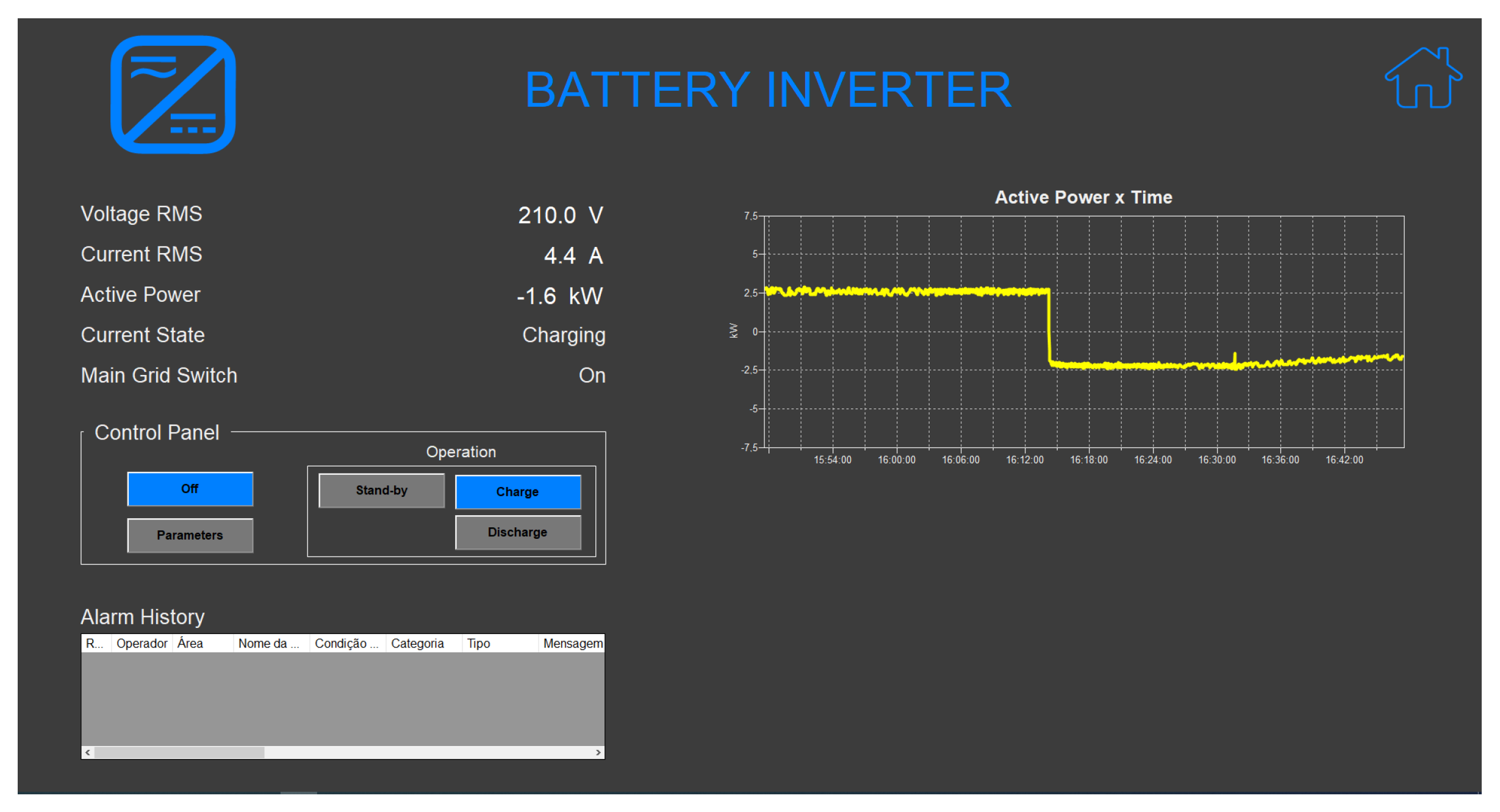
The supervisory system also includes auxiliary screens that provide information about each of the components and have some control functionalities. As an example, the figure displays the screen related to the inverter that interfaces between the battery bank and the microgrid. It can be observed various electrical quantity information that the equipment is exposed to, its current operational status, as well as some command buttons. These buttons allow the change in the operational state of the equipment, which includes standby, charging, and discharging modes. The button related to parameters enables the configuration of the amount of current to be injected into the microgrid and set references for battery charging, which include the reference current for the constant current mode and the reference voltage for the constant voltage mode during the charging process of the batteries.

The screen shown in Figure 33 also includes a graph displaying the variation of power over time. As observed, initially, the inverter operated in discharge mode, injecting about 2.5 kW for approximately 30 minutes. After this period, the inverter switched to battery charging mode, drawing approximately (−2.5 kW). It is worth noting that after about 18 minutes of charging operation, the power drawn by the converter starts to decrease, indicating that the charging process has transitioned from the constant current mode to the constant voltage mode.

It is important to note that each of the agents that make up the microgrid has its own supervision and control screen. However, due to space constraints, they are not presented. All measurement data related to the microgrid equipment are stored in the MS SQL Server, making it possible to generate operational reports of the microgrid and identify the time at which a specific alarm associated with one of the monitored equipment occurred.

5. Conclusions and Future Work

This article addresses a significant gap in current research by presenting a scaled-down laboratory dedicated to the development and testing of hardware and software associated with power electronics-based devices in the context of microgrids. The focus on industrial applications distinguishes this work from contemporary studies, which predominantly center around microgrids within the system and integration domain. The laboratory was designed to encompass elements that are gaining prominence in the current microgrid landscape, such as renewable generation, storage systems, electrolyzers for $H_2$ production, and cogeneration sources.

Given that communication systems are a crucial component in the context of microgrids associated with smart grid philosophy, a supervisory system was developed to meet the demands of studies in these areas applied to microgrids. The supervisory system aims to monitor and coordinate various agents within the microgrid. The developed structure provides an effective and robust initial platform for conducting future studies regarding intelligent decision-making algorithms for the operational optimization of these networks.

Regarding power electronics-based devices, a converter was developed for controlling a storage system, which also operates as a grid-forming unit in the event of microgrid islanding. Additionally, a boost converter was developed to simulate a cogeneration system based on thermal generation through devices that convert thermal energy into electrical energy via the Seebeck effect. The sizing process of these converters and the algorithms associated with their functionality were detailed, and the presented results demonstrated effective operation in meeting the initial demands of the laboratory.

With the equipment developed in addition to the supervisory system, the microgrid can detect and act in the event of grid islanding. Doing so is a challenge to overcome, given the difficulty of overcoming equipment security systems.

Also, the exploration of non-traditional cogeneration sources, such as electrolyzers and thermoelectric generator (TEG) systems, contributes to a more comprehensive understanding of microgrid dynamics. The integration of an electrolyzer and the decision to connect DC-based components to an AC bus offer valuable insights into the challenges and considerations related to these components’ incorporation into microgrids. This paper provides detailed insights into the laboratory setup, control loops, and operational results, emphasizing the development of non-commercial devices.

In summary, the laboratory presented in this article proves to be a powerful tool for studies focused on microgrids, as it is capable of encompassing the key components and issues related to these systems. The developed structure has shown versatility in conducting studies related to converter control algorithms. Therefore, with the developed laboratory, it will be possible to make improvements in the functionalities already described, as well as implement new features such as compensation for harmonic currents and reactive power.