1. Introduction
Nitrogen oxides, generally known as NOxs, are some of the most important hazardous air pollutants from industry [
1,
2]. In China, the NOx emission in the waste gas of industrial sources was about 8.957 million tons in 2022 [
3]. When emitted into the atmosphere, NOx undergoes a series of photochemical reactions with volatile organic compounds under the UV light of sun radiation to generate irritating photochemical smog [
4,
5]. NOx also reacts with O
2 and H
2O to form acid rain [
6]. NOx in the stratosphere is believed to be an important ozone depletion substance, damaging the ozone layer protecting our eco-system [
7]. With the rapid increase in the growth of the economy and energy demand, the total amount of anthropogenic NOx emitted in the world has increased by three–six times [
8], bringing massive hidden dangers to the ecological environment and human health.
Previous research has revealed that the majority of annual ambient NOx emissions could be attributed to fossil fuel combustion, especially coal combustion in power plants [
9]. In China, many efforts have been made to control the NOx emission from coal-fired power plants. Over 90% of Chinese coal-fired power plants have completed the installation of selective catalytic reduction (SCR) technology to reduce their NOx emission [
10].
However, the existing SCR technology is facing a dilemma that the detection of NOx concentrations cannot keep up with the fluctuation in the NOx concentrations in flue gas due to the sample extraction process which is conducted before the NOx reaches the gas analyzer. The NOx concentration fed to the distributed control system (DCS) is usually several minutes behind the actual NOx variation in the flue gas. Therefore, it is very difficult for the ammonia injection system to quickly respond to the NOx concentration fluctuation to achieve better NOx removal. Most power plants inject excessive ammonia into the SCR reactor to be sure that the NOx finally emitted to the atmosphere is below the government-permitted limit. This strategy will inevitably increase the cost of SCR operation and the chance of ammonia slipping into environment.
To address the inherent delays in traditional NOx measurement, non-contact instantaneous measurement technologies were developed. However, in flue gas environments, dust interference is significant, and laser measurement technology requires precise alignment of the angle of incidence. Their high susceptibility to dust interference can lead to damage to expensive measurement instruments, hence their limited application in power plants.
In situations where improvements in hardware measurement are not feasible, we consider using soft-sensing methods to address the aforementioned issues. An accurate online NOx concentration prediction method for soft sensors is essential in improving the performance of SCR systems, as soft sensors can be used as the feedforward signal for SCR control to make up for the inherent delay problem in the existing NOx measurement, and to control the ammonia injection in advance to achieve the effect of accurate denitrification in the power plant.
NOx prediction can be divided into mechanism-driven and data-driven methods. Many previous efforts have been made to develop NOx mechanism models. Many mechanism models on NOx formation have been proposed using fitting combustion [
11,
12,
13,
14] and flow processes [
15,
16,
17]. Thomas Le Bris et al. [
18] established computational fluid dynamics simulations for a 600 MW pulverized coal unit, and validated their prediction by NOx reduction via over-fire air. Unfortunately, these mechanism models are too complicated for SCR process control. The formation and transportation of NOx couples chemical reactions and flow processes [
19]. The prediction of NOx concentrations at the SCR inlet is either unreliable without the accurate simulation of the in-furnace coal combustion process and downstream flow process [
18], or very slow if reaction and flow parameters included. Therefore, it is almost impossible at the moment to build a mechanism model to cope with the requirements of online operation.
By contrast, with the fast development of industrial digitalization [
20,
21], the massive data generated in power plants every day [
2] may contain a lot of information not known to us yet. Fully excavating and making good use of these data might be immensely helpful in regulating the SCR control using a different aspect.
In recent years, the artificial intelligence aided by machine learning and big data technologies has been rapidly applied to the power industry [
22,
23,
24,
25,
26,
27]. Wang et al. [
28] proposed a Gaussian process (GP) to fit the NOx emission characteristics with 21 boiler parameters, and identified the optimal parameters to predict boiler combustion and NOx emission. Zhou et al. [
29] built an artificial neural network (ANN) model for NOx emission based on 12 sets of experimental data of a 600 MW unit, with the influences of over-firing air, secondary air, nozzle tilt, and coal properties on NOx combustion characteristics being investigated. A modified genetic algorithm (GA) was developed to optimize the combustion conditions for NOx reduction. Adams et al. [
30] developed LSSVM and DNN models to predict the SOx and NOx emissions associated with coal conversion in a CFB power plant. Yang et al. [
31] treated NOx concentrations as a time-series problem and applied a long-short term memory (LSTM) neural network to model NOx emission. Wang et al. [
32] proposed a prediction method of NOx emission and mass flow rate before the SCR of diesel vehicles based on mutual information (MI) and reversed back propagation neural network (BPNN). The above methods demonstrated the effectiveness and potential of industrial data prediction in a data-driven way.
The above literature summarizes relevant studies in the field of industrial NOx emission prediction, primarily employing methods such as artificial neural networks (ANNs), deep neural networks (DNNs), long short-term memory (LSTM) networks, and Gaussian processes. These studies have trained and tested their models on various datasets, achieving a certain level of predictive accuracy.
However, the following limitations remain:
- 1.
Reliance on single data-driven methods: Most studies rely solely on data-driven machine learning approaches, without considering the physical mechanisms of NOx formation, which may result in limited generalization capabilities of the models;
- 2.
Poor model interpretability: While deep learning models such as DNN and LSTM demonstrate high predictive accuracy, their “black-box” nature reduces the interpretability and trustworthiness of the models, posing challenges for practical engineering applications;
- 3.
Inapplicability in real-time operations: The aforementioned deep learning models involve complex convolutional computations, whereas DCS systems in coal-fired power plants are limited to simple operations. As a result, these models are difficult to deploy on-site, rendering them unsuitable for real-time use;
- 4.
Limited prediction lead time: Some studies do not account for the need to predict NOx emissions ahead of time, thereby failing to provide sufficient adjustment time for process control.
Necessity of this Study:
In light of these limitations, our research aims to integrate mechanistic models with data-driven models to develop a soft-sensing model capable of predicting NOx emissions in coal-fired power plants with physical interpretability and a lead time of 3 min. By combining knowledge of NOx-generation mechanisms with advanced machine learning algorithms, we seek to improve the predictive accuracy and generalization ability of the model, enhance its interpretability, and provide more effective technical support for NOx reduction and control in coal-fired power plants.
This approach not only addresses the shortcomings of purely data-driven models but also ensures that the weak learners used are deployable on-site. Moreover, the ensemble learning method mitigates the risk of gradient explosion and delivers more reliable predictive results, meeting the demands of practical engineering applications for NOx emission control.
In fact, NOx concentration is an industrial variable containing the characteristics of data series and coupling with industrial data itself. The existing research has rarely combined the actual power plant combustion process with the data-driven coupling relationship.
This study aims to bridge this gap by combining the characteristics of industrial time-series data on NOx concentrations with boiler operation parameters related to the formation and transport mechanisms of NOx. The objective of this paper is to propose a forecasting model that can achieve a lead time of up to three minutes, enabling its online application in power plants as an advanced soft measurement sensor which can compensate for the measurement delays of the existing hardware. To develop a robust online 3 min advanced NOx prediction model for power plants, this study will be structured around three main objectives:
Development of a new indicator: We introduced a novel indicator, PR2. This indicator focuses on the model’s predictive accuracy at turning points, filling gaps left by other indicators and providing a specific evaluation of the model’s applicability in industrial settings.
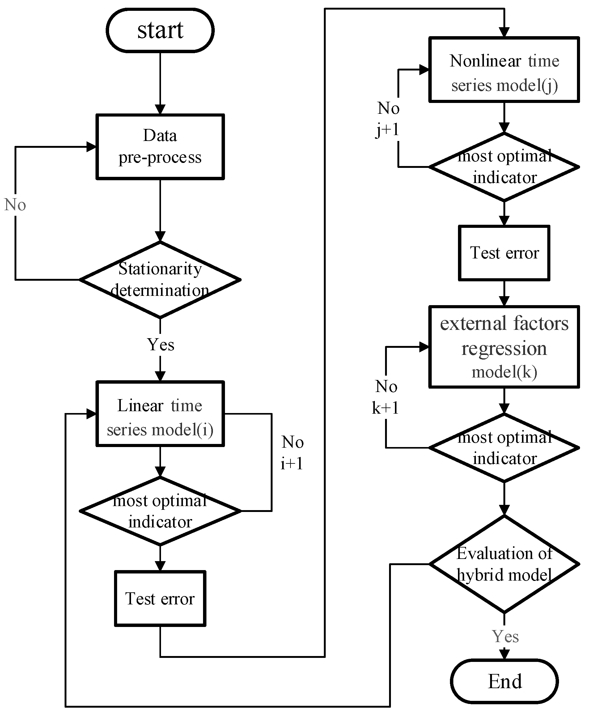
Three-layer integrated prediction method: This study proposed a three-layer integrated framework that categorizes industrial data from a power plant into stable time-series features, volatile time-series features, and external features related to the combustion side. The integrated hybrid prediction algorithm was then developed to accurately forecast NOx concentrations.
A time-based method for analyzing the correlations between variables in the denitration systems and NOx concentrations: By utilizing big data analysis, we investigated the time delays between various exogenous variables related to combustion and the NOx concentrations, as well as the exact measurement delays in an actual power plant.
The predictive model in this paper will be trained offline. To enable deployment in the plant’s DCS system, we integrated a simplified model. Once trained and implemented in the control system, no additional training time or computational resources will be required. The model will simply function as a feedforward signal, as shown in
Figure 1, to optimize the control system. The proposed model will be used as the
ufeedforward signal in the denitrification control process shown in
Figure 1, predicting changes in NOx concentration in advance and enabling timely ammonia injection to ensure precise NH
3 concentrations.
4. Prediction Results
4.1. Feature Selection
In coal-fired power plants, the NOx concentrations involve a variety of complex reaction mechanisms. These mechanisms represent the fundamental characteristics of NOx and are essential for the “interpretability” required by computer models or big data analyses. Due to the complexity of mechanistic models, which often precludes their online application, this paper combined big data time-series features with mechanistic insights to construct a joint NOx prediction model. The incorporation of multivariate mechanistic features significantly enhanced the robustness of the model, avoiding the significant errors and biases typical of simpler univariate models.
In this study, the actual physical process model was mined from the data by the maximal information coefficient (MIC) feature selection of combustion variables involved in the front end. The front-end influence variables included air-side, coal-side, and other variables which had been verified by the MIC to be influential on the NOx concentration. The results of the feature extraction were as follows.
Figure 6 reveals that the variables exhibiting a strong correlation with the NOx concentration include the total coal amount, primary and secondary air flows,
, and outlet air temperatures, as well as the SCR inlet and outlet flue gas temperatures. For instance, in
Figure 6a, the primarily selected variables relate to air flows, including secondary air flow on the left side of the furnace and on the right side of the furnace. In
Figure 6b, the selected variables include the total coal quantity, actual unit load, instantaneous coal feed from the coal feeder, flue gas temperature (variables 123), oxygen content, and pressure difference between the inlet and outlet of the flue gas, which were consistent with existing research on NOx formation mechanisms. These strongly correlated variables selected by both the mechanism model and the data model will participate in the subsequent prediction.
In addition to traditional feature analysis, this study incorporated time-delayed variables into the model. Each variable was intentionally shifted by varying time delays to examine its correlation with the NOx concentration. This approach not only corroborated the actual measurement delays experienced in the power plant but also aided in determining the realistic time delays for different variables.
Figure 7 revealed that the optimal delay times between the different variables and the NOx concentrations were not the same. Meanwhile, an interesting phenomenon can be observed, that all variables showed optimal delay times around 2–3 min, which corresponded to the previously analyzed potential 3 min delay in NOx measurements at this power plant. This finding confirmed that we can quantitatively describe the temporal delays between the variables and NOx concentrations through data analysis. It also aided in analyzing the measurement delays of NOx at the plant to design an effective advance prediction model. This represented a significant innovation, providing a solid foundation for future NOx prediction in power plants. This method enhanced the predictive accuracy of our NOx concentration model by aligning it more closely with the dynamic operational conditions of the plant.
4.2. Prediction Results
Due to the long sampling line and the analysis time required for the NOx measurement process in power plants, there is usually a delay of several minutes in the measurement session. The delay time in the power plant in this study was calculated by data and correlation analysis to be approximately 3 min. Therefore, this section will apply the exogenous variables identified through feature selection and a three-tiered prediction approach to forecast real-time data from power plants. The effectiveness of the model’s predictions will be evaluated using the multiple indicators previously discussed and compared. Moreover, since the existing predictive studies typically focus on one-minute single-step predictions, to validate the advantages of the proposed model over the existing methods, this study also conducted single-step one-minute predictions and three-step three-minute predictions.
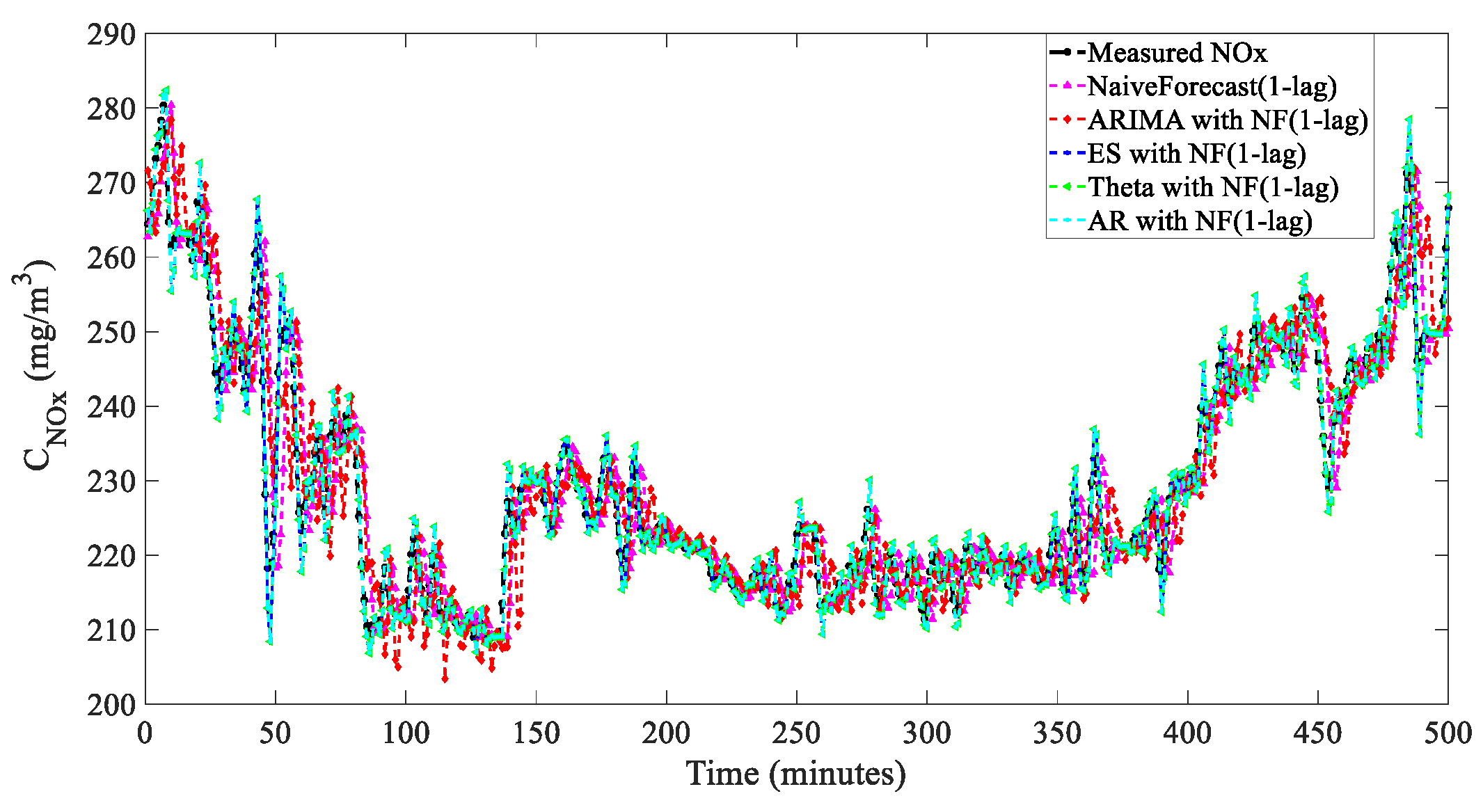
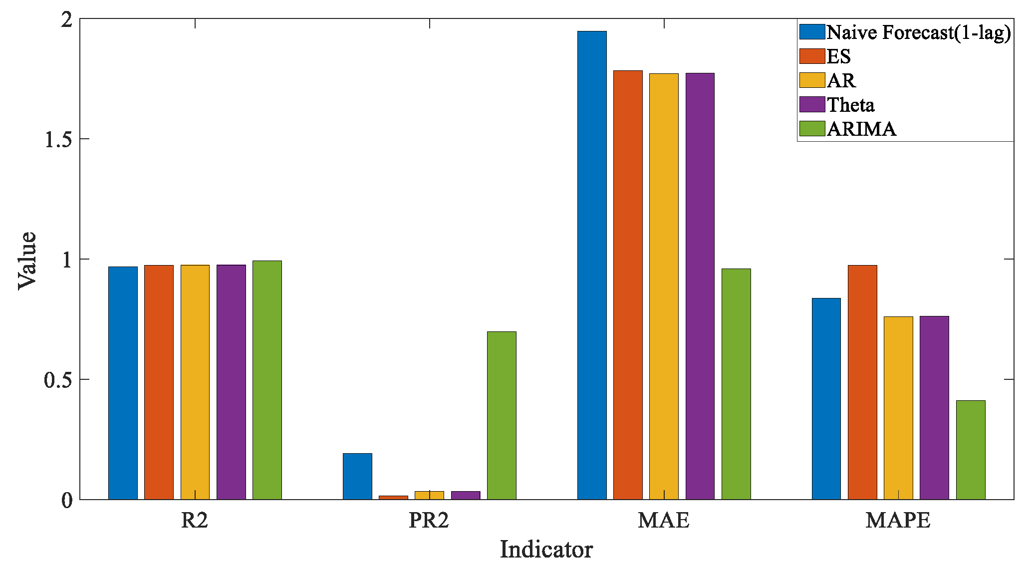
It can be seen from
Table 3 and
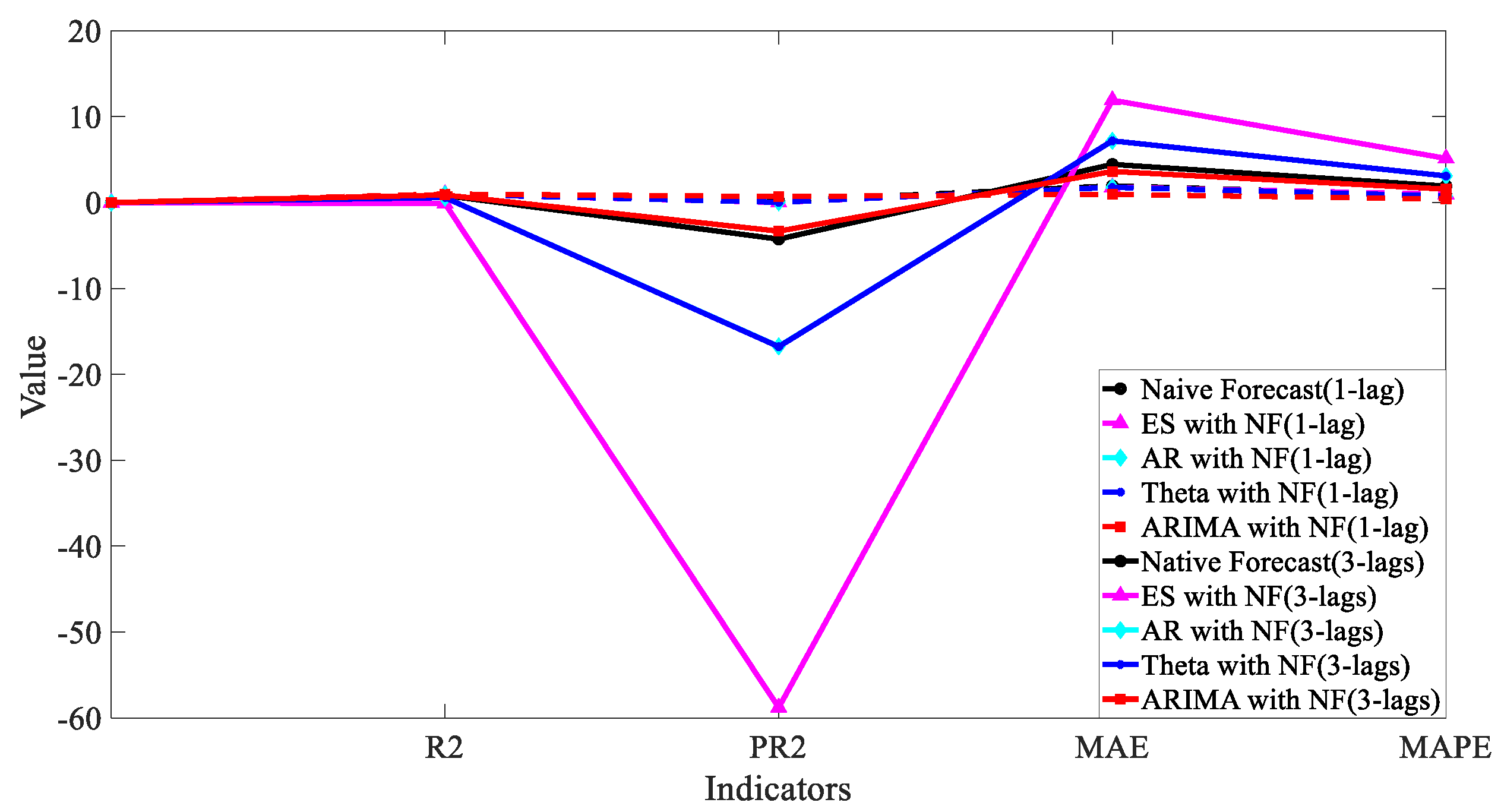
Figure 10, that, in 1 min prediction, ARIMA (1-lag) had the best prediction among the linear time-series models above. At the same time, the one-minute prediction combined with (NF 1-lag) can greatly improved the effect of the model prediction, and it showed that the data trend was more important in the single-step prediction. Moreover, we can see that the performances of different models on different evaluation indicators were not corresponding. For instance, the Naive Forecast model had a better PR2 value and a worse MAE value when compared with those of AR and Theta models. Therefore, we need to choose a prediction model that better meets our needs. The proposed PR2 might distinguish itself the traditional models when using another aspect.
In the 3 min prediction, as shown in
Figure 14, the ES (NF3) and AR (NF3) models were diverged. Despite several adjustments to the parameters of both models, the divergence persisted, likely due to the ES and AR models functioning by applying different weighted accumulations to prior NOx concentrations. This mechanism was akin to an open-loop model without feedback. In the three-minute forecasts, the NF-3 (without feedback) combination disrupted the original model, significantly increasing the probability of divergence. For other models, as the forecasting interval extended to three minutes, the amount of useful information contained diminished. The overall performance of the linear time-series forecasting models deteriorated, especially when they were combined with native prediction models. This deterioration may be due to the inaccuracies represented by the three-lag data that the original predictive model cannot rectify. Consequently, we rearranged the three-minutes multi-step forecasts using a linear regression algorithm alone, the results of which are presented below.
Table 5 and
Figure 15,
Figure 16,
Figure 17 and
Figure 18 revealed that, with the exception of the ARIMA algorithm, the ES, AR, and Theta methods showed significant improvements in their 3 min prediction performance when not combined with the NF (3-lag) feature. However, despite the ES model’s R
2 score improving from −0.126 to 0.64, it still exhibited considerable bias in its predictions. This issue likely stemmed from the intrinsic nature of the ES model as primarily a data smoothing technique, which may not be well-suited for multi-step predictions over a short 3 min interval. Additionally, the ES model’s inherent lag and limited ability to recognize turning points further contribute to its substantial bias in calculations.
In our analysis of linear models, the ARIMA model demonstrated the highest prediction accuracy at one-minute prediction for both turning points and overall average levels. However, as the prediction interval increased to three minutes, the performance of the linear time-series models generally declined. This suggested that most of the predictive information at the one-minute mark can be effectively extracted from the inherent patterns of the time-series itself. ARIMA showed an advantage in modeling short-term predictions where the series is relatively smooth.
For three-minute predictions, there appeared to be a greater need for information about nonlinear or external physical processes. Notably, the ARIMA model maintained its robustness across the different linear prediction models tested, showing little variation in performance whether combined with the NF3-lag feature or not. This indicated that the moving average component of the ARIMA model played a crucial role in stabilizing the predictions. Based on these observations, we selected the ARIMA model as the linear baseline model for integrating subsequent nonlinear and regression models in our predictive framework. This choice was supported by ARIMA’s proven effectiveness in handling predictions and its robust performance under varying conditions.
- (1)
Prediction of nonlinear time-series models
The application of nonlinear models in our study primarily addressed the local volatility within the time-series that the linear models were unable to manage effectively. The linear models were best-suited for series that display stable expectations and variance. However, if a series exhibits variance changes—as observed in our dataset—models like ARCH and its derivatives were found to be more apt for addressing these fluctuations.
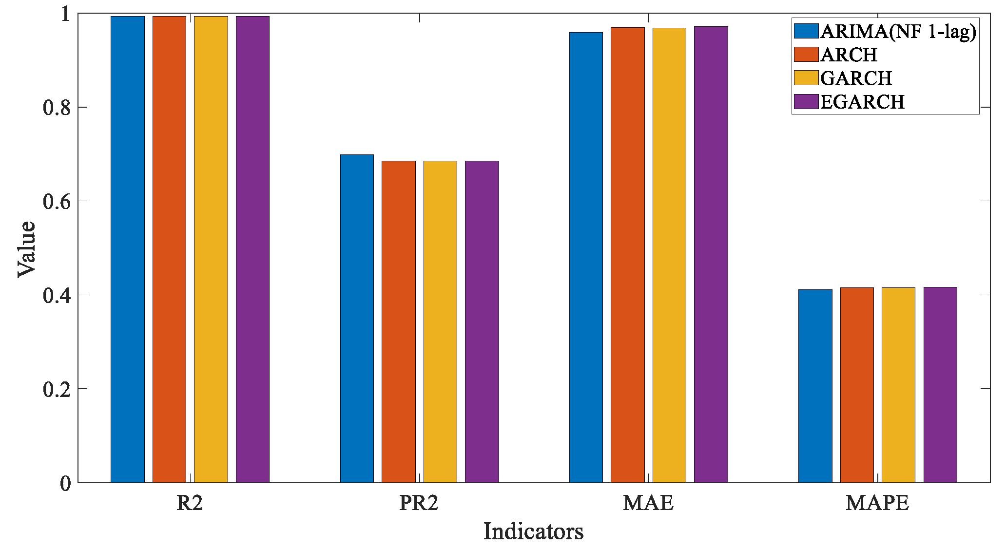
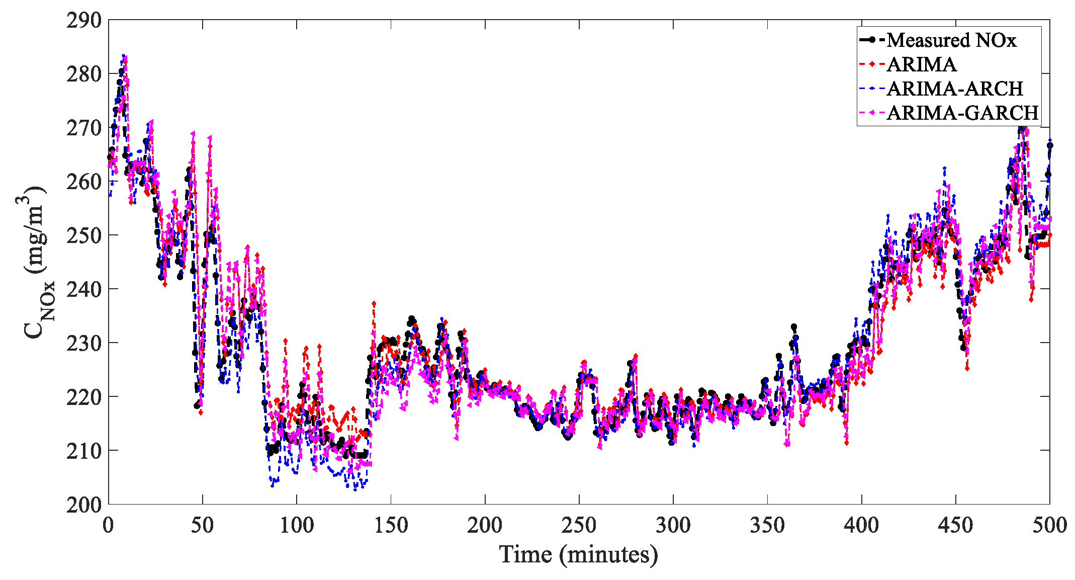
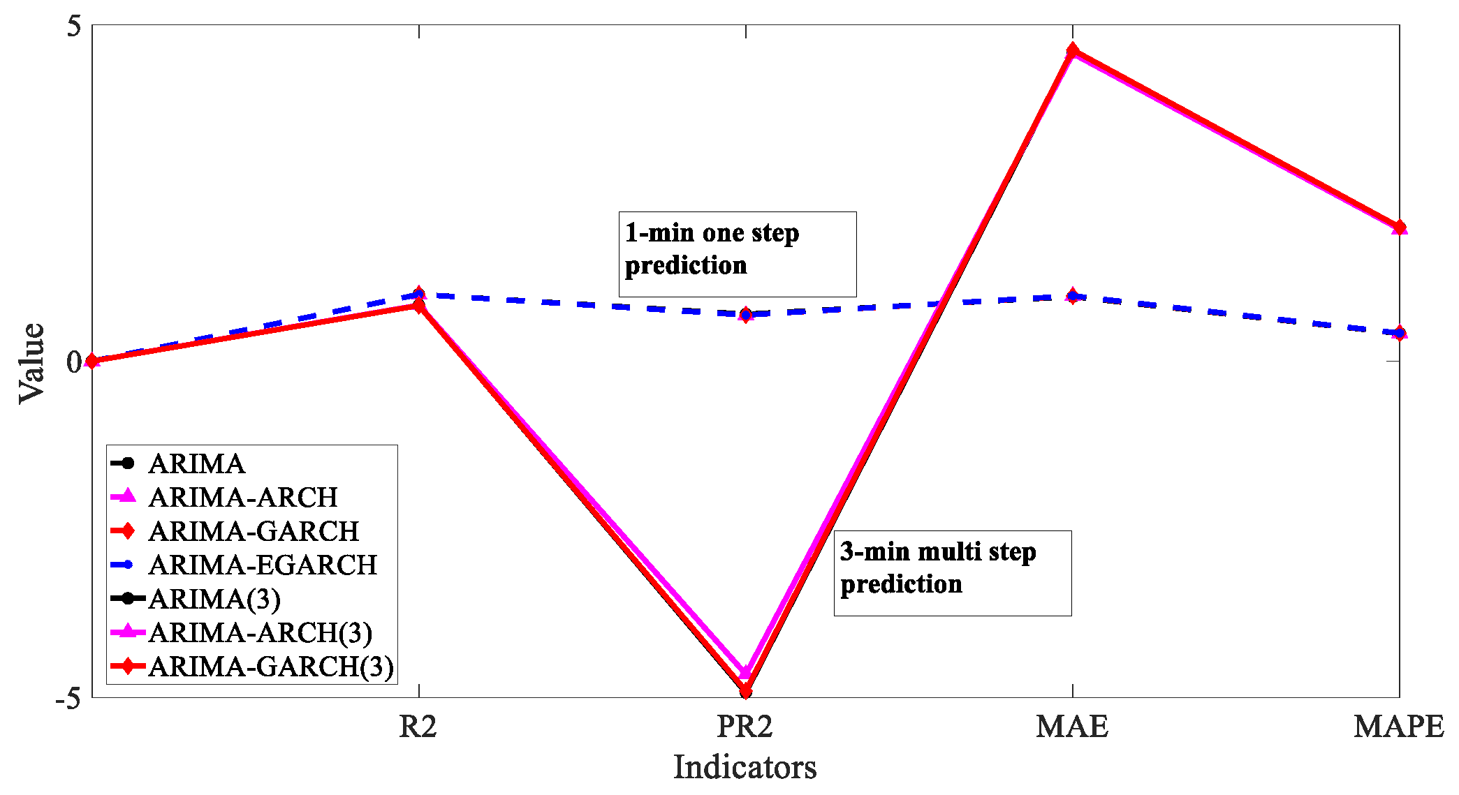
In this study, we employed several nonlinear models, including ARCH, GARCH, and EGARCH, to handle the complexities of the dataset where linear models fall short. To enhance the prediction accuracy, we integrated these nonlinear models with the ARIMA linear model. The hybrid model indicators of ARIMA and the nonlinear models were as follows.
From the data presented in
Table 6 and
Figure 19,
Figure 20,
Figure 21,
Figure 22,
Figure 23 and
Figure 24, it was evident that the use of nonlinear models in one-minute, short-term, single-step predictions did not enhance the overall accuracy of the models; instead, it may lead to overfitting. This suggested that, for short prediction intervals, maintaining model simplicity can be more beneficial.
In the above
Figure 19,
Figure 20,
Figure 21,
Figure 22,
Figure 23 and
Figure 24 and
Table 7, detailing the forecasting effect of the combined nonlinear model, it can be seen that the forecasting evaluation indicators such as the R
2 and PR2 of the combined model were improved after the addition of the nonlinear model. The PR2 indicator in the pooled ARCH model was improved the most, indicating that ARCH improved the forecasting effect of the combined model through variance compensation. It also confirmed its effectiveness in dealing with local fluctuations.
- (2)
Prediction of multivariate regressive time-series models
In this part, we delineated the models as follows. These models, despite varied mechanisms, shared essential characteristics common to regression models used in statistical learning. This part of the prediction utilizes multivariate regression based on highly correlated variables identified through the feature selection of front-end variables in
Section 4.1 The model continued to extract information related to mechanistic models from the operational data, thereby further enhancing the overall predictive performance of the integrated model.
This part of the prediction primarily fitted the weights of different independent variables by reducing residuals and the loss function. Compared to the linear and nonlinear time-series predictions discussed earlier, this prediction was multivariate and included information related to the NOx generation mechanism model. In the power plant experiments, we also adaptively adjusted the weights of these independent variables based on the NOx generation mechanism.
Table 8 and
Table 9 below show the effect of NOx concentration prediction by combination models for the 1-min and 3-min, respectively.
As can be seen in
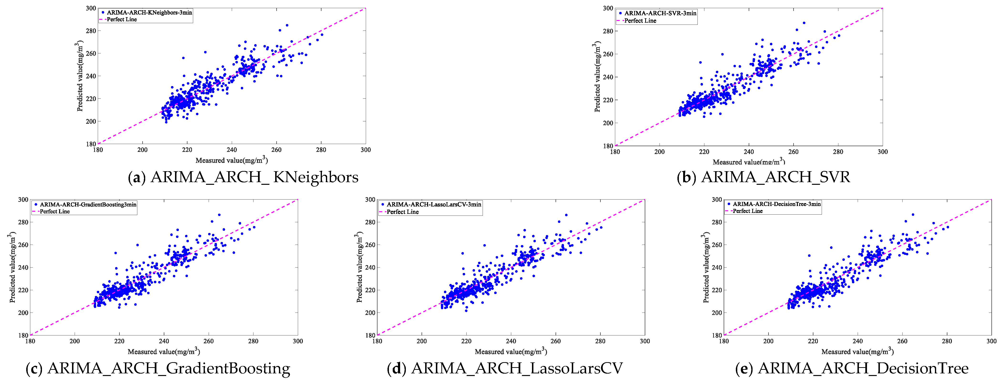
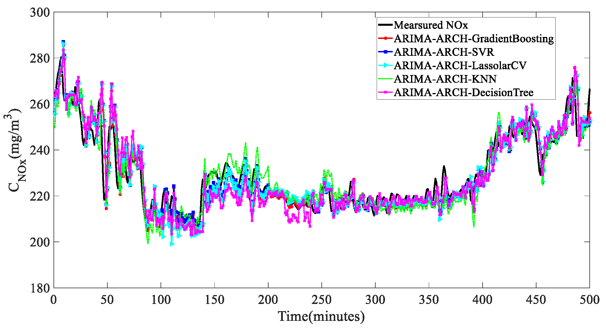
Table 8, the combined models are all accurate for 1-min predictions. For the 3-min prediction, there is some difference in the effectiveness of the combined model, and
Figure 25 and
Figure 26 show the 3-min prediction of the combined model.
The above analysis indicated that, for short-term predictions of one minute, the trend information in the time-series data was relatively important for forecasting. The additional benefits of combining nonlinear or regression models were minimal.
However, for multi-step predictions over three minutes, where the data were resampled at one-minute intervals and then used to predict the concentrations three minutes later, there was an excessive loss of trend information, leading to a decreased forecasting performance. In this case, combining the NOx generation mechanism model with the nonlinear factors of the data will enhance the overall predictive performance.
Our findings highlighted that a composite model, which integrated linear time-series, nonlinear time-series, and exogenous regression models, demonstrates significant advantages in three-minute multi-step forecasts. Notably, in our dataset, the ARIMA_ARCH_GradientBoosting model emerged as the most effective for three-minute predictions. This model adeptly combined the strengths of individual forecasting techniques, optimizing the predictive accuracy and reliability, which are essential for operational efficiency in power plant settings. Therefore, the ARIMA_ARCH_GradientBoosting model will be employed as the proposed model in this study for subsequent tests of generalizability and comparison with the existing literature.
4.3. Generalizability Testing
In applying the prediction models to industrial processes, the most important concern was the generalization of the model. In this study, based on the previous model, predictions were made on an untrained data segment from the same power plant, and the prediction results are shown in
Figure 27:
The results, illustrated in
Figure 27, demonstrated that the model effectively predicts NOx levels over a three-minute interval, maintaining a high accuracy even with new data. The smoother characteristics of this data segment yielded an R
2 score of 0.9115, which was superior to the previous result of 0.8463 obtained from a different segment. This improvement confirmed the model’s robust generalization performance across varying data conditions.
To compare the three-minute prediction accuracy of the proposed combination boosting model with existing predictino models, this study employed a widely used deep learning approach, the long short-term memory (LSTM) model. The LSTM network is a variant of recurrent neural networks that is specifically designed to process and predict event-related characteristics in time-series data. It is commonly used in fields such as time-series analysis and forecasting. For the LSTM model, we employed a two-layer architecture with 100 and 50 units, respectively, to extract and learn complex time-series relationships. For training, we chose the Adam optimizer with an initial learning rate of 0.01. A dropout rate of 0.2 was implemented to reduce overfitting of the model, and the output layer neurons were selected as 1 and 3 for the single- and three-step predictions, respectively. In single-step forecasting, the LSTM model resulted in an R2 value of 0.9902, a PR2 value of 0.6770, an MAE of 1.0743, and a MAPE of 0.4842. It can be observed that, in single-step prediction using the LSTM model, due to the absence of a residual compensation process, the prediction accuracy at turning points is somewhat inferior. To achieve more precise predictions from the data, the LSTM model can be further optimized through a boosting strategy to enhance its accuracy at turning points. However, since this study was intended for on-site application, one-minute or LSTM predictions can only serve as comparative models and were not suitable for subsequent on-site application. Under these conditions, the prediction model proposed in this paper will possess the strongest adaptability and robustness. Since the ultimate goal of this study is to propose a set of 3 min advance prediction combination models that will be available in the field, we applied the LSTM model to the selected data segments for 3 min prediction; the prediction outcomes are presented below.
Figure 28 shows a comparison between the final proposed combined prediction model and the LSTM model, specifically for time-series prediction, where the R
2 of the proposed integrated model was 0.8463, the R
2 of the LSTM model was 0.82102, and the PR2 of the LSTM model was −4.4832, which made us realize that deep learning and complex models are not a panacea, and that specific analysis methods for specific data were more meaningful and effective. We believe the superior predictive performance of the model proposed in this paper, compared to related work, is due to continuously optimizing the PR2 metric during the process and the ability to adjust the parameter k in the PR2 based on different data and prediction requirements. Additionally, our familiarity with the NOx formation mechanism allowed us to make specific parameter-weight adjustments in the ARIMA model based on this mechanism.
More importantly, compared to related studies, the key advantage of the approach proposed in this paper is that it can be implemented on-site. Additionally, it predicts NOx concentrations 3 min ahead, meaning that this is not simply an optimization of a prediction model in the field of computer science, as the reviewer suggested, but rather a practical, deployable model designed to solve real-world problems. Consequently, it is challenging to perform a detailed comparison with existing studies. Furthermore, we introduced the PR2 parameter, tailored to practical applications, and proposed an ensemble learning model based on multiple weak learners, incorporating data characteristics and the conditions of on-site applications. These innovations improve the overall predictive performance, serving as an optimized feedforward for the SCR control systems in power plants.
Additionally, this study opted for a combination of simpler models primarily because such an approach is feasible for implementation in a power plant setting, unlike deep convolutional neural networks which may not be practical on-site. This decision underscores the importance of model applicability in real industrial environments.
4.4. Discussion
In this section, we will analyze the model’s performance in terms of accuracy, robustness, and applicability to real industrial scenarios. We will compare the predictive performance of the proposed model with that of existing studies and the LSTM model.
In one-minute single-step predictions, the trend information in the time-series data dominated the forecast, and incorporating additional models at this stage may cause overfitting, reducing the prediction effectiveness. In contrast, in three-minute multi-step predictions, the trend information was greatly reduced, and the inclusion of the naive forecast model degraded the predictive performance, while incorporating the data’s inherent nonlinearities and the physical generation mechanisms of NOx can enhance the reliability of the predictions.
In this study, the proposed model was applied to actual data from a 330 MW power plant, showing excellent predictive accuracy. For 3 min prediction, compared to predictions made by ARIMA, the fitting degree R
2 and the PR2 were increased by 3.6% and 30.6%, respectively, and the MAE and MAPE were decreased by 9.4%, and 9.1%, respectively. It can also be observed that the PR2 evaluation indicator proposed in this paper provided a sharper contrast than traditional indicators. For example, in
Table 1, the difference in R2 values between the predictions is minimal, while the difference in the PR2 is significant, indicating that the PR2 offers more distinct prediction results. In
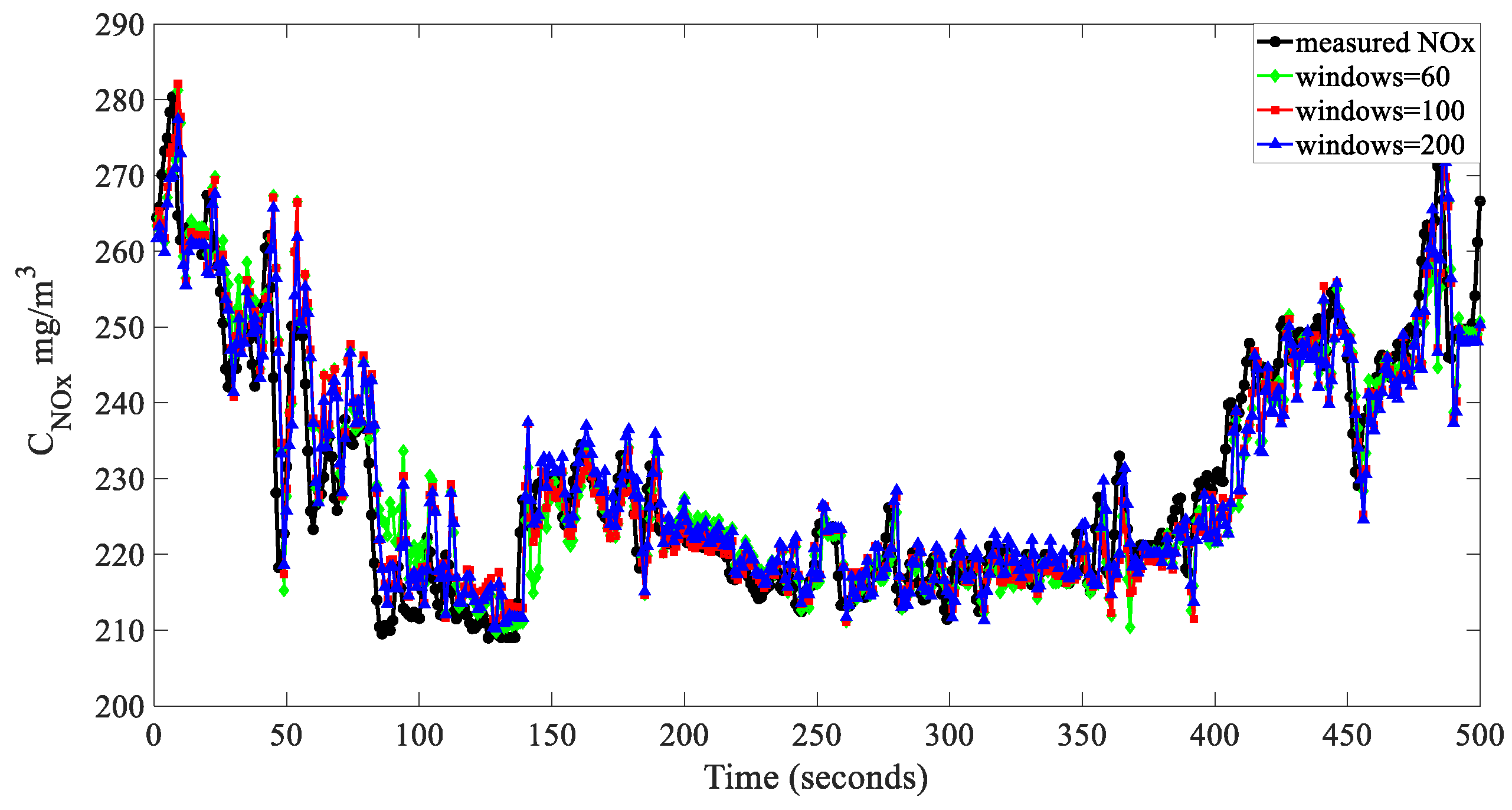
Table 2, the traditional prediction indicators were improved with longer window lengths, whereas the PR2 exhibited a turning point, making it easier to select model parameters and window lengths.
Additionally, existing research on NOx prediction has introduced a method combining random forest and just-in-time learning for forecasting NOx concentrations in thermal power plants [
43], achieving a maximum R2 of 0.9319 and a MAE of 2.7718. These figures were lower than those reported in our study, with an R2 of 0.9925 and a MAE of 0.4213. This further substantiated the effectiveness of the method proposed in our paper for enhancing predictive accuracy.
In addition, we also conducted predictions using an LSTM model with the same data and, for comparison, the R2 of the proposed model for 3 min prediction is 0.8463, whilst that of the deep learning LSTM model for 3 min prediction is 0.82102. This comparison illustrates that deep learning and complex models are not universally optimal. Tailored analytical methods specific to the data can be more meaningful and effective. More importantly, the field implementation of NOx advance prediction is made possible by the combination of a simple prediction model with a boosting method.
The error analysis can be directly observed in
Figure 22,
Figure 26, and
Figure 28, as well as similar figures. Even though the PR2 parameter was introduced, the model still cannot entirely avoid the inherent shortcomings of prediction models, particularly showing poorer performance when there are large fluctuations in the data. While the introduction of the PR2 parameter offers some improvement over other models in terms of optimization during significant data variations, this remains a common issue in data prediction. Therefore, this is an area for future work, where further advancements in data modeling will allow for more improvements in predictive soft-sensing. On the other hand, since the prediction data in this paper were downsampled to minute-level data, the model’s performance in handling data with jagged fluctuations still requires further improvement.
5. Conclusions and Future Work
To address the issue of delays in online NOx measurement in power plant denitration processes, this study introduced a hybrid boost integration model suitable for on-site implementation at power plants. The forecasting method proposed in this paper aims to achieve a lead time of up to three minutes for forecasts, enabling its online application in power plants as an advanced soft measurement sensor. This advanced forecasting method, when applied in coal-fired power plants, will serve as a feedforward signal in the SCR control system, applied to the ammonia injection valves. It can act as a soft measurement model to compensate for the inherent hardware measurement lag, aligning the control signals with the measurement signals and enhancing the efficiency of precise ammonia injection.
- (1)
This study introduced a new evaluation indicator, PR2. This indicator focuses on the model’s predictive accuracy at turning points, filling gaps left by other traditional indicators and providing an evaluation different from traditional parameters in data prediction, enhancing the model’s predictive performance;
- (2)
A time-based method was proposed for analyzing the correlations between variables in denitration systems and NOx concentrations. Using this method, we investigated the time delays between various exogenous variables related to combustion and the NOx concentrations, as well as the exact measurement delays in an actual power plant;
- (3)
To address the issue of NOx measurement delays, this study introduced a hybrid boosting model suitable for on-site implementation. This model combined generation mechanism and data-driven approaches, enhancing prediction accuracy through the categorization of time-series data into linear, nonlinear, and exogenous regression components. These results confirmed the accuracy and applicability of the integrated model for on-site implementation as a 3 min advanced prediction soft sensor in power plants.
In this paper, we have introduced a novel metric, PR2, tailored specifically for industrial prediction, proposed an ensemble learning model that integrates multiple weak learners and is deployable on-site, and identified the correlation between NOx concentration and upstream combustion and flow-side variables with respect to the time delay. These three innovations represent significant contributions to NOx soft-sensing in coal-fired power plants, as no prior work has addressed these aspects. Importantly, all of our innovations are aimed at solving real-world problems, and the approach outlined in this paper has already been successfully implemented at a power plant.
In the future, given the similarities between many industrial processes and the denitrification stage of coal-fired power plants—such as defined generation mechanisms and limited hardware conditions—the methods proposed in this paper can be directly applied to related industrial processes. Furthermore, the ensemble learning approach introduced here provides valuable insights for using data and weak learners to maximize information extraction and enhance data prediction under constrained industrial conditions. At the same time, the proposed soft-sensing predictive algorithm has already been applied in a real coal-fired power plant, achieving promising results.
Of course, there are still several areas for improvement in this paper. For example, with the further development of mechanistic models and big data technologies, the accuracy of our three-minute-ahead predictions could be improved. Additionally, predicting the NOx concentration across the flue cross-section in the SCR control stage of coal-fired power plants is also an important aspect. However, the plant currently lacks NOx data for its flue cross-section. These issues are expected to be addressed in future developments, which will collectively enhance denitrification efficiency.

