Article

Advanced Machine Learning Techniques for Energy Consumption Analysis and Optimization at UBC Campus: Correlations with Meteorological Variables

by
Amir Shahcheraghian
* and
Adrian Ilinca
*
Department of Mechanical Engineering, École de Technologie Supérieure, Montreal, QC H3C 1K3, Canada
*
Authors to whom correspondence should be addressed.
Energies 2024, 17(18), 4714; https://doi.org/10.3390/en17184714
Submission received: 31 August 2024 / Revised: 13 September 2024 / Accepted: 20 September 2024 / Published: 22 September 2024
(This article belongs to the Special Issue Energy Efficiency and Energy Performance in Buildings)

Abstract

:
Energy consumption analysis has often faced challenges such as limited model accuracy and inadequate consideration of the complex interactions between energy usage and meteorological data. This study is presented as a solution to these challenges through a detailed analysis of energy consumption across UBC Campus buildings using a variety of machine learning models, including Neural Networks, Decision Trees, Random Forests, Gradient Boosting, AdaBoost, Linear Regression, Ridge Regression, Lasso Regression, Support Vector Regression, and K-Neighbors. The primary objective is to uncover the complex relationships between energy usage and meteorological data, addressing gaps in understanding how these variables impact consumption patterns in different campus buildings by considering factors such as seasons, hours of the day, and weather conditions. Significant interdependencies among electricity usage, hot water power, gas, and steam volume are revealed, highlighting the need for integrated energy management strategies. Strong negative correlations between Vancouver’s temperature and energy consumption metrics are identified, suggesting opportunities for energy savings through temperature-responsive strategies, especially during warmer periods. Among the regression models evaluated, deep neural networks are found to excel in capturing complex patterns and achieve high predictive accuracy. Valuable insights for improving energy efficiency and sustainability practices are offered, aiding informed decision-making for energy resource management in educational campuses and similar urban environments. Applying advanced machine learning techniques underscores the potential of data-driven energy optimization strategies. Future research could investigate causal relationships between energy consumption and external factors, assess the impact of specific operational interventions, and explore integrating renewable energy sources into the campus energy mix. UBC can advance sustainable energy management through these efforts and can serve as a model for other institutions that aim to reduce their environmental impact.

1. Introduction

In 2018, global building emissions increased by 2% for the second consecutive year, reaching 9.7 gigatons of carbon dioxide (GtCO2) [1]. This marks a shift from the trend observed between 2013 and 2016, when emissions stabilized. Floor space and population growth have led to a 1% rise in energy consumption in buildings, reaching 125 exajoules (EJ), which constitutes 36% of the global energy use [1]. Academic buildings on a typical UK university campus cover about 42% of the total area and are responsible for nearly 50% of the campus’s energy consumption and carbon emissions [2]. Predicting energy usage in these buildings has become increasingly important for facility managers, aiding energy planning and regulation [2]. Accurate forecasting can reveal potential energy savings and support energy conservation efforts on campuses [3]. However, energy consumption is influenced by various factors, including meteorological conditions, electromechanical system operations, and holiday schedules, making predictions challenging due to the inherent nonlinearity and uncertainty [3].
There are two main approaches for predicting building energy consumption: physical and data-driven models [4]. Physical models analyze buildings based on physical principles, but require extensive data and long simulation times, making them complex and less efficient. In contrast, data-driven models use historical data to predict energy consumption, and are known for their flexibility, ease of data acquisition, and accuracy [5].
This study evaluates different data-driven models, including machine learning and deep learning techniques, to assess their effectiveness in predicting the energy consumption of campus buildings. Specifically, it compares various machine learning models (e.g., Decision Tree, Random Forest, Gradient Boosting) and neural networks (ANN) across 167 buildings on the UBC Campus. The analysis examines the prediction accuracy using metrics such as MAE and R2 scores, providing insights into the performance of these models.
The goal of this article is to conduct a detailed analysis of energy consumption within UBC Campus buildings using a range of machine learning models, including Neural Network, Decision Tree, Random Forest, Gradient Boosting, AdaBoost, Linear Regression, Ridge Regression, Lasso Regression, Support Vector Regression, and K-Neighbors. This study explores how different factors—such as season, time of day, and meteorological conditions—affect energy consumption patterns. This research uses sophisticated analytical methods to uncover and quantify the complex relationships between energy demand and environmental factors. The findings of this research offer valuable insights for improving energy efficiency, sustainability practices, and informed decision-making for energy management in educational campuses and similar urban settings.
A fundamental knowledge gap in energy consumption analysis lies in the limited accuracy of traditional models and their inability to fully capture complex interactions between energy usage and meteorological data. Conventional approaches often fail to account for the intricate, nonlinear relationships between environmental factors and energy demand, leading to suboptimal predictions and reduced effectiveness of energy management strategies. Addressing this gap requires the application of more advanced models that can better understand these dynamic interactions, ultimately improving forecasting accuracy and energy optimization efforts.
To conduct a detailed analysis of the energy consumption within UBC Campus buildings using various machine learning models, it is crucial to examine the challenges faced in previous studies and highlight the need for more advanced techniques. One of the primary issues identified in earlier research is the reliance on relatively simple statistical models, which, while more straightforward to implement, often fall short of capturing the full complexity of energy consumption dynamics. For instance, Khuram Pervez Amber et al. [6] developed a forecasting model using Multiple Regression (MR) to predict the daily electricity consumption in university buildings based on six explanatory variables, including ambient temperature, solar radiation, and building type. Although the model achieved promising results, with a Normalized Root Mean Square Error (NRMSE) of 12% and 13% for two different building types, it struggled to account for the deeper nonlinear interactions between these variables. The study emphasized the need for more reliable and flexible models to accommodate a broader range of buildings and capture more complex relationships between variables.
Similarly, Sadeghian Broujeny et al. [7] outlined the challenges in forecasting building energy consumption due to the intricate management of multiple influencing parameters. Their work demonstrated the effectiveness of artificial intelligence (AI) models, such as Long Short-Term Memory (LSTM) and Gated Recurrent Unit (GRU), achieving an RMSE of 0.23. However, they also highlighted the need to select optimal time lags and exogenous data to enhance the model performance. While these AI models provide superior predictive accuracy, challenges remain in managing model complexity and extracting meaningful historical knowledge from a wide range of features.
These studies underscore the knowledge gap in developing models that can accurately forecast energy consumption while capturing the complex nonlinear interactions between meteorological variables and energy usage. To explore these interdependencies more effectively, this article aims to bridge this gap by employing various machine learning models, including Neural Networks, Decision Trees, Random Forests, and Gradient Boosting. In doing so, this study sets out to establish new baseline accuracy levels and address the limitations of prior work, where simpler models or narrowly focused AI techniques may have missed critical patterns in energy consumption. Applying these advanced models will provide a more comprehensive understanding of how factors, such as temperature, time of day, and seasonal variations, influence energy use in campus environments, thereby establishing a new benchmark for future research.

2. Literature Review and Background

Lei et al. [8] developed a prediction model for building energy consumption by integrating rough sets with deep learning, utilizing a data-driven and adaptive control scheme. Their model combines the rough set theory, which uses a genetic algorithm-based attribute reduction method to eliminate redundant factors, with a deep belief network (DBN) for information recognition. This hybrid approach significantly improves the prediction accuracy for both short-term and medium-term energy consumption compared to traditional neural networks like BP, Elman, and fuzzy neural networks. The use of rough set theory reduces the number of inputs, thereby enhancing the performance of the DBN. This advancement highlights the potential of machine learning to create accurate building energy simulations, thereby enabling more effective real-time power supply scheduling and demand management.
Fan et al. [9] explored the effectiveness of deep learning techniques for predicting building cooling loads, comparing them with state-of-the-art prediction methods and feature extraction techniques. They found that deep learning methods, particularly nonlinear techniques like extreme gradient boosting (XGB), outperformed linear methods. The best performance was achieved using XGB models with features extracted by unsupervised deep learning models such as deep autoencoders. Interestingly, supervised deep learning models did not require complex architectures; a shallow model with two hidden layers sufficed, likely due to dataset size and inherent patterns. This study underscores the value of unsupervised deep learning in feature extraction, which consistently improves the prediction accuracy over conventional methods. The proposed deep learning-based techniques offer precise 24-h-ahead cooling load predictions, which help build operation management, demand-side management, optimal control strategies, and fault detection. Future research should explore diverse data sources to validate and expand on these methods.
Jui-Sheng Chou et al. [10] reviewed machine learning techniques for energy consumption forecasting in buildings using real-time smart grid data. They highlighted the effectiveness of hybrid models that combine forecasting and optimization techniques, demonstrating improved accuracy and usability for energy management planning. This review contributes to advancing energy efficiency and sustainable development efforts.
Carla Sahori Seefoo Jarquin et al. [11] examined five university buildings to create day-ahead load forecasts using feed-forward neural networks trained with a similar day method. They classified data into low, medium, and high consumption categories and evaluated ten models per category against benchmarks. Most models exceeded benchmarks and met ASHRAE accuracy standards, with notable improvements from incorporating features like seasonal shifts, day-night cycles, and recency effects. Models M3, M9, and M10 were remarkably accurate. Despite the robust point forecasts, the prediction intervals from the dynamic ensemble approach were too narrow, suggesting the need for alternative methods. This research indicates the potential for extending forecasts to include heat demand, various facility types, smart cities, and energy communities, emphasizing hierarchical forecasting for better collective energy management.
Bo Han et al. [3] analyzed the use of support vector machine (SVM), Gaussian process regression (GPR), and decision tree (DT) models for predicting campus building energy consumption. Their comparative study found that the SVM model achieved the highest prediction accuracy, outperforming the GPR model by 5.79% and the DT model by 13.93%. This study demonstrated the feasibility and effectiveness of the SVM model in accurately predicting the electricity consumption in campus buildings, highlighting its superiority over other prediction methods.
Bilal Akbar et al. [2] investigated two data-driven forecasting techniques, artificial neural networks (ANN) and multiple regression (MR), to estimate daily electricity usage at London South Bank University. Using historical data from 2007 to 2011, they analyzed the impact of five different climate factors on energy consumption. They found that energy consumption is highly influenced by the Weekday Index, a proxy for building occupancy, and Dry Bulb Temperature. ANN outperformed MR, achieving mean absolute percentage error (MAPE) values of 2.44% for working days and 4.59% for non-working days. Both techniques performed well; however, the ANN demonstrated a slight advantage. This research provides a foundation for predictive studies in other building categories and offers valuable insights for energy managers seeking to accurately forecast building energy usage patterns. The findings suggest that predictions remain reliable over time if the building operates under the same schedule.
Linas Gelažanskas et al. [12] analyze hot water power data from residential buildings to develop and test various forecasting models, including exponential smoothing, SARIMA, and seasonal decomposition. The results show that these models outperform simpler benchmarks, with seasonal decomposition being the most effective at improving forecast accuracy. This work highlights the significance of advanced predictive techniques for enhancing demand-side management and supporting grid stability in the context of increasing renewable energy integration.
Jinyuan Liu et al. [13] review 70 years of gas consumption forecasting, categorizing the evolution into four stages: initial, conventional, AI, and all-round. They highlight that time series models excel in long-term forecasting with a mean absolute percentage error of 1.90%, and support vector regression models (4.98%) are more suitable for short-term forecasting. This review emphasizes the impact of computer science and AI advancements on forecasting performance and proposes a framework for model selection along with future research directions.
Predicting gas volume, electricity, and hot water power consumption on campuses poses several challenges that Machine Learning (ML) and Artificial Neural Networks (ANN) can address effectively. Regarding gas volume consumption, issues include the impact of seasonality and weather, varying usage patterns across buildings, and data sparsity. ML and ANN models can address these challenges by integrating weather data and using regression techniques to correlate consumption with the relevant features. Electricity consumption prediction is complicated by complex load patterns, demand fluctuations, and the need to account for multiple factors, such as HVAC systems and lighting. Advanced ML models, including ANN, can enhance the prediction accuracy. Similarly, predicting hot water power consumption involves addressing the challenges related to temperature variability, usage patterns, and system dynamics. Employing predictive models, making seasonal adjustments, and incorporating system performance data can improve the accuracy. Overall, effective data preprocessing, feature selection, and model evaluation are crucial for developing robust and accurate consumption predictions.

3. Research Methodology

3.1. Data Collection

The data collection for this study utilizes the UBC Energy & Water Services’ online live data, accessible through the SkySpark platform [14]. This platform is part of the campus as a Living Lab initiative, and offers valuable insights into building energy and performance metrics. SkySpark, developed by Skyfoundry, is an Internet of Things (IoT) platform that leverages heating, ventilation, air conditioning (HVAC), and energy data to enhance building performance [15].
Since 2017, the Energy & Water Services’ Energy Conservation team has used SkySpark to monitor and optimize building control systems and identify energy and greenhouse gas (GHG) savings opportunities. The platform supports the long-term storage of a substantial amount of data, including 68,000 data streams, 370 energy meters across 167 campus buildings, 5000 pieces of HVAC equipment, and 3 Building Management Systems (BMS) vendors [16].
For this study, data from 2023 were collected, encompassing hourly profiles from 1 January to 31 December. This comprehensive dataset provides a detailed view of energy consumption and performance metrics across various building types and functions on the UBC campus, as illustrated in Figure 1.

3.2. Data Pre-Processing

The initial phase of the study involves collecting a diverse range of data frames crucial for analyzing energy consumption:
  • Time-Dependent Data Frames: Capturing temporal patterns in energy usage.
  • Non-Time-Dependent Data Frames: Providing static information about building characteristics.
  • Weather Data Frames: Offering environmental context, including meteorological conditions.
  • Electricity Energy Data Frames: Detailing power usage across the campus.
  • Gas Volume Data Frames: Indicating gas consumption patterns.
  • Hot Water Energy Data Frames: Tracking hot water usage.
  • Steam Volume Data Frames: Recording steam consumption.
  • Water Volume Data Frames: Monitoring general water usage.
  • Total Data Frames: Consolidating comprehensive building energy data for each building in the target year 2023.
This extensive dataset establishes the foundation for subsequent analysis.
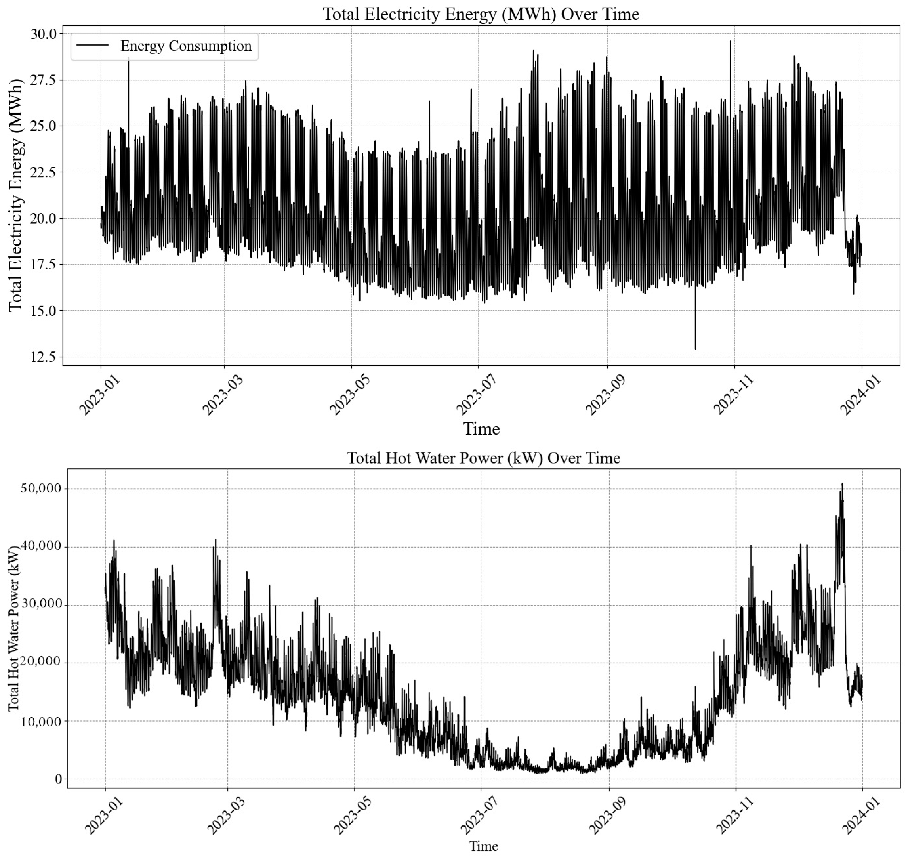
Following data collection, rigorous data cleaning procedures ensure data integrity and reliability. Figure 2 illustrates the total electricity energy and hot water power consumption across the campus for 2023. Outliers for Electrical Energy and Hot Water Power are identified and removed from crucial data frames to prevent skewed results and enhance predictive accuracy. Data quality checks are also performed on weather and electrical energy data frames to eliminate any NaN (Not a Number) values, ensuring the dataset is complete and reliable.
The decision not to use pipelines and transformers for preprocessing was based on the specific requirements of this study, which focused primarily on energy consumption forecasting. While pipelines and transformers can streamline preprocessing tasks and ensure a consistent workflow, this study employed a more targeted approach for data cleaning and outlier removal using tailored procedures such as the Interquartile Range (IQR) method to ensure the reliability of the dataset.
Outliers were estimated using the IQR method, which is a robust statistical approach commonly applied to detect and remove extreme values from a dataset. The IQR method calculates the difference between the third quartile (Q3) and the first quartile (Q1), identifying outliers as any data points lying below Q1—1.5 * IQR or above Q3 + 1.5 * IQR. This method was chosen because of its simplicity and effectiveness in dealing with energy consumption data, where occasional extreme values can significantly distort model performance.
Before outlier deletion, the dataset comprised 8760 rows, representing hourly data for the entire year. After applying the IQR method, 31 outliers were removed, resulting in a final dataset of 8729 rows. This minimal reduction in data ensures that the dataset remains comprehensive while improving the overall quality and accuracy of the subsequent machine learning models. By focusing on high-quality data, the models developed in this study can capture the energy consumption patterns and their dependencies on meteorological variables more accurately.
A total value column is added to each data frame to view the energy consumption comprehensively. This column aggregates the energy consumption for each hour by summing the values across all buildings, thereby providing a consolidated overview of energy usage patterns.
Following preprocessing, a range of machine learning models, including Neural Network, Decision Tree, Random Forest, Gradient Boosting, AdaBoost, Linear Regression, Ridge Regression, Lasso Regression, Support Vector Regression, and K-Neighbors, are applied to the cleaned dataset.
The selection of machine learning models for this study was driven by the need to address the complex and nonlinear relationships between energy consumption and meteorological variables as well as to compare a range of model types to determine the most effective approach. Each model was chosen based on its ability to handle different aspects of the data and the challenges of energy consumption forecasting.
The Neural Network (ANN) was selected for its ability to model intricate, nonlinear relationships between energy consumption and environmental factors like temperature and wind speed. ANN flexibility, especially with multiple layers and the use of nonlinear activation functions such as tanh, makes it particularly effective for datasets with both positive and negative inputs, capturing complex patterns in the data. Decision Trees were chosen for their interpretability and capability to manage nonlinear interactions between features, making them useful for understanding how variables such as time of day and seasonal changes impact energy usage.
Building on Decision Trees, Random Forest was included for its ability to reduce overfitting by averaging predictions across multiple trees, resulting in more accurate and stable forecasts across buildings with varying consumption patterns. Gradient Boosting and AdaBoost, both ensemble methods, were chosen for their superior performance through the iterative improvement of weak learners. Gradient Boosting is particularly well-suited for regression tasks, providing high accuracy in predicting energy consumption, while AdaBoost focuses on difficult-to-predict instances, helping to refine predictions.
To compare against more complex models, Linear Regression, Ridge Regression, and Lasso Regression were selected as simpler models. Linear Regression serves as a baseline, while Ridge and Lasso offer regularization techniques to prevent overfitting by penalizing large coefficients, providing insights into how well linear assumptions hold in this context. Support Vector Regression (SVR) was chosen for its ability to handle both linear and nonlinear relationships by applying the kernel trick, making it suitable for capturing the dependencies between energy usage and meteorological factors in high-dimensional spaces. SVR is also robust to outliers, and generalizes well to smaller datasets.
Lastly, K-Neighbors Regression was selected as a non-parametric model that predicts energy consumption based on the behavior of nearby data points, offering a simple yet effective method for capturing local patterns in energy usage. By employing this diverse set of machine learning models, this study seeks to identify the most effective approaches for accurately forecasting energy consumption while accounting for the complex interactions between variables, ultimately providing a more comprehensive understanding of energy patterns in campus environments.
In the training process, the database consists of 8760 rows, representing hourly data for the entire year of 2023. The measurements were recorded on an hourly basis throughout this period. The dataset was initially cleaned and preprocessed, and then divided into three subsets: 70% for training, 15% for validation, and 15% for testing. The training set was used to fit the models, allowing each algorithm—Neural Network, Decision Tree, Random Forest, Gradient Boosting, AdaBoost, Linear Regression, Ridge Regression, Lasso Regression, Support Vector Regression, and K-Neighbors—to learn patterns and relationships within the data by adjusting their internal parameters to minimize training error. During the training, a portion of the training data was set aside as a validation dataset to fine-tune the hyperparameters and prevent overfitting. This validation process involved assessing the model performance on this subset and making adjustments to improve the generalization. After training and validation, the models were evaluated on a 15% testing set, which remained unseen during the training and validation phases. This evaluation assessed the models’ ability to generalize to new, unseen data, with performance metrics such as MAE, MSE, RMSE, and R2 being calculated to determine their accuracy and effectiveness. This method ensures that the models’ predictive performance is realistically measured against the data they have not been exposed to during training and validation.
All hyperparameters utilized for the ML models in this project are detailed in Table 1.
Special attention is given to the Artificial Neural Network (ANN) hyperparameters, which significantly impact the model accuracy. The ANN used in this study features multiple layers: an initial Dense layer with 128 neurons and a tanh activation function, followed by layers with 64, 64, and 32 neurons, all of which utilize the tanh function. The output layer consists of a single neuron for regression purposes. The ‘tanh’ activation function was chosen for its ability to introduce nonlinearity into the model, which is crucial for capturing complex patterns in energy consumption data. It outputs values between −1 and 1, centering the data and helping to address the vanishing gradient problem. Additionally, ‘tanh’ handles negative inputs effectively, which aligns with the characteristics of our dataset. This choice helps improve the model’s learning dynamics and performance. All the hyperparameters utilized in this project are detailed in Table 2.
A dropout rate of 0.4 was implemented following each BatchNormalization layer to mitigate overfitting. This technique randomly sets a fraction of input units to 0 during training updates, enhancing model robustness. Additionally, L2 regularization with a factor of 0.01 was applied to the weights of the second, third, and fourth Dense layers. This penalizes large weights and further reduces the risk of overfitting.
The Nadam optimizer was utilized, combining the advantages of Adam and Nesterov momentum with a learning rate of 0.0005 to optimize the model’s performance. To fine-tune the learning rate, the ReduceLROnPlateau callback was employed. This callback reduces the learning rate by half if the validation loss does not improve for 10 epochs, with the minimum learning rate set to 10−6.
A batch size of 16 was chosen to provide a regularizing effect and improve generalization. The model was trained for 10 epochs to balance the risks of overfitting and underfitting. A custom callback, TestLossCallback, was used to monitor the test loss at the end of each epoch, offering additional insight into the model’s performance on the test set. Through careful selection and tuning of these hyperparameters, the ANN was optimized for better performance and generalization, with each hyperparameter playing a crucial role in enhancing the model’s predictive capabilities.
Applying machine learning models and meticulous tuning of ANN hyperparameters are vital for capturing complex relationships within the dataset, thus providing valuable insights for optimizing energy systems.
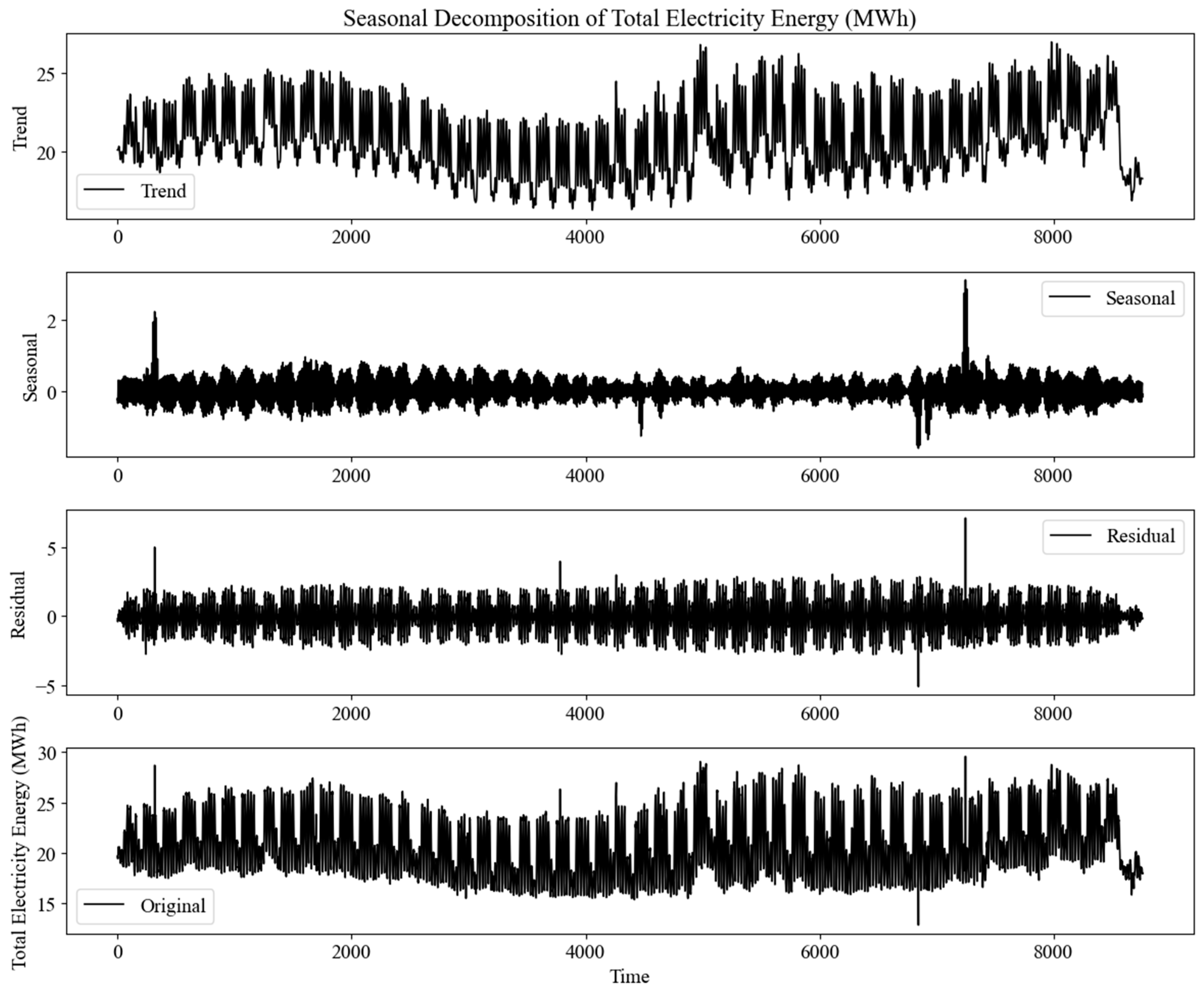
Additionally, data preparation included Decomposition Analysis to uncover the underlying trends, seasonality, and residual patterns in energy consumption data. Decomposition involves breaking data into three components: trend, seasonality, and residuals [18]. The trend component shows long-term changes in the energy consumption, such as increases or decreases. Seasonality captures recurring patterns, such as daily or monthly fluctuations due to weather or operational schedules. Residuals represent random fluctuations or noise not explained by the trend or seasonality [19].
Figure 3 illustrates the trend of electricity energy, seasonal, and residual components. Analyzing these residuals helps identify unpredictable elements in energy consumption and informs strategic decision-making, including peak consumption periods, resource optimization, and accurate future energy demand predictions.

3.3. Model Testing and Evaluation

The methodology involves extensive testing and evaluation of various forecasting models to assess their performance in predicting the energy consumption. This includes applying different regression methods, such as decision tree regression, to test the models across multiple years. This approach allows for a thorough evaluation of the predictive accuracy over different time frames.
To determine the effectiveness and reliability of each model, several performance metrics are used:
  • R-squared (R2): This statistic measures the proportion of variance in the dependent variable (energy consumption) explained by the independent variables (features) in the model. It ranges from 0 to 1, with higher values indicating a better fit between the model and data. A higher R-squared value means that the model accounts for a more significant proportion of the variance in the target variable, reflecting better explanatory power. Despite its benefits, R2 should be interpreted cautiously and in conjunction with other metrics to avoid overestimating model performance. Similar studies, including [7], have employed R2 to understand the model’s ability to capture the variability in energy consumption.
R 2 = 1 i = 1 n y i y ^ i 2 i = 1 n y i y ¯ 2
y i is the actual value of the dependent variable.
y ^ i is the predicted value of the dependent variable.
y ¯ is the mean of the actual values of the dependent variable.
n is the number of observations.
  • Mean Absolute Error (MAE): MAE quantifies the average magnitude of errors between actual and predicted values, providing a clear indication of model accuracy. For instance, similar studies by [3,20] utilized MAE to benchmark model performance in energy forecasting tasks. Lower MAE values signify more accurate predictions, indicating that the model predictions are closer to the actual values. The advantages of MAE are its simplicity and ease of interpretation; however, it does not penalize larger errors more than smaller ones.
M A E = 1 n i = 1 n y i y ^ i
  • Root Mean Square Error (RMSE): RMSE measures the square root of the average squared difference between actual and predicted values. This metric emphasizes more significant errors than MAE, as it penalizes larger discrepancies more heavily. Lower RMSE values indicate better model performance, with minor deviations from the actual values. Its application in previous works, such as [21], underscores its effectiveness in evaluating model accuracy, although it shares the disadvantage of sensitivity to outliers.
R M S E =   1 n i = 1 n ( y i y ^ i ) 2
By analyzing these metrics, the methodology evaluates each model’s efficacy in capturing energy consumption patterns and provides insights into their predictive accuracy.

4. Results

4.1. Correlation between the Parameters

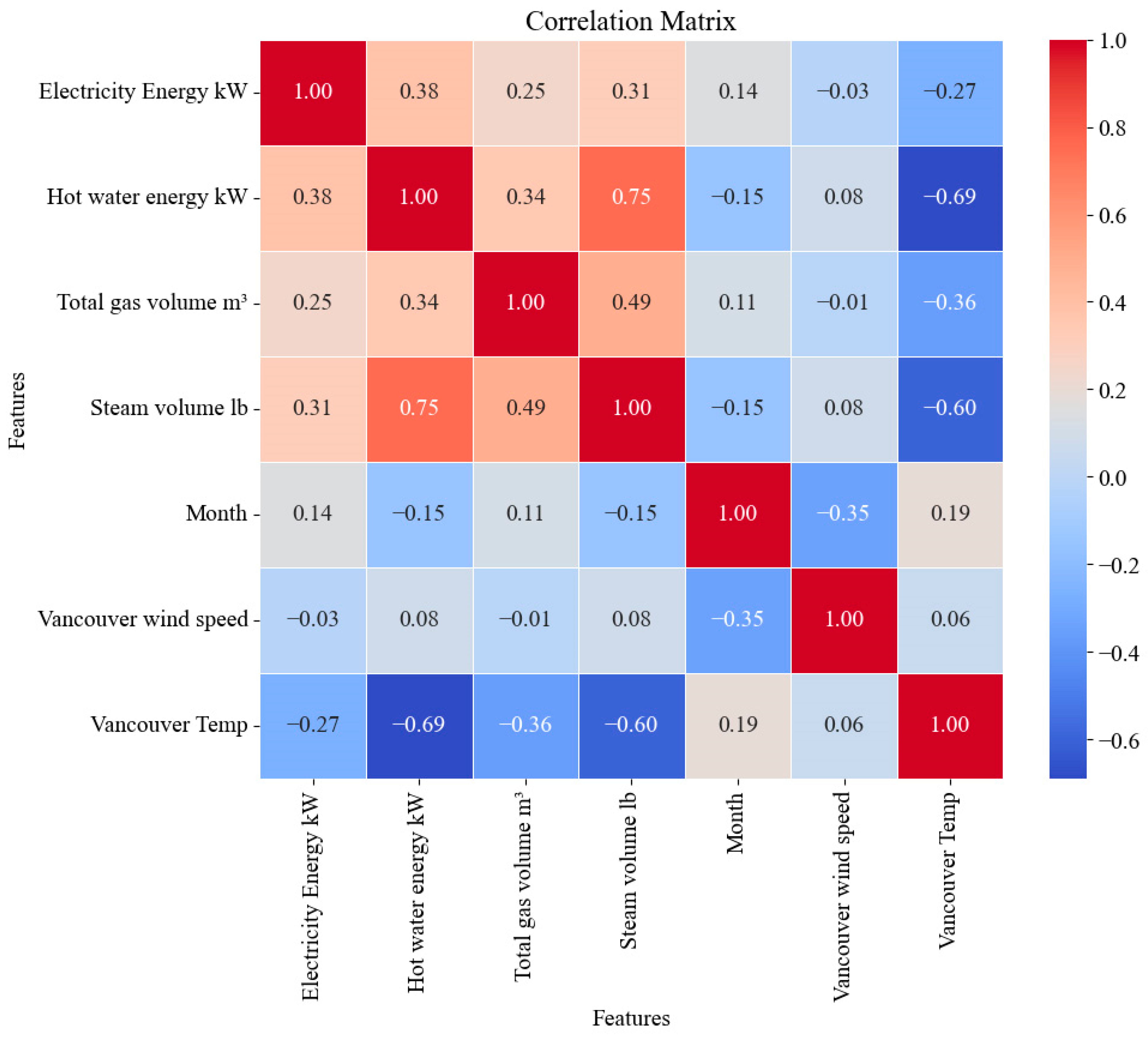
The correlation analysis depicted in Figure 4 for the UBC University campus in Vancouver reveals several significant relationships among various energy consumption metrics. Notably, the correlation between electricity energy usage and hot water power consumption is 0.38, indicating a moderate positive association where increases in electricity use are moderately related to increases in hot water power consumption. In contrast, the correlation between electricity energy and gas volume is weaker at 0.25, suggesting that changes in one may not strongly impact the other. A moderate positive correlation of 0.31 between electricity energy and steam volume shows a notable relationship between these two metrics.
The analysis (Table 3) also highlights a strong positive correlation of 0.75 between the hot water power and steam volume, which is likely attributed to the implementation of the UBC’s medium-temperature hot water system in 2017 [22]. Furthermore, the correlation between hot water power and gas volume is 0.34, indicating a moderate positive relationship. Gas and steam volumes exhibit a moderate positive correlation of 0.49, suggesting a considerable relationship between these variables.
Seasonal effects show a weak positive correlation of 0.19 with temperature, reflecting a mild influence of seasonal variations on temperature fluctuations. Strong negative correlations are observed between temperature and energy consumption, with values of −0.69 for hot water power and −0.60 for steam volume, indicating that warmer temperatures are associated with reduced energy usage for these metrics. A moderate negative correlation of −0.27 is noted between temperature and electricity energy consumption, suggesting a less pronounced but noticeable reduction in electricity use during warmer periods. These correlations offer valuable insights into how energy consumption patterns interact with steam management and environmental factors at the UBC campus, aiding the development of effective energy optimization and sustainability strategies.

4.2. Electrical Energy

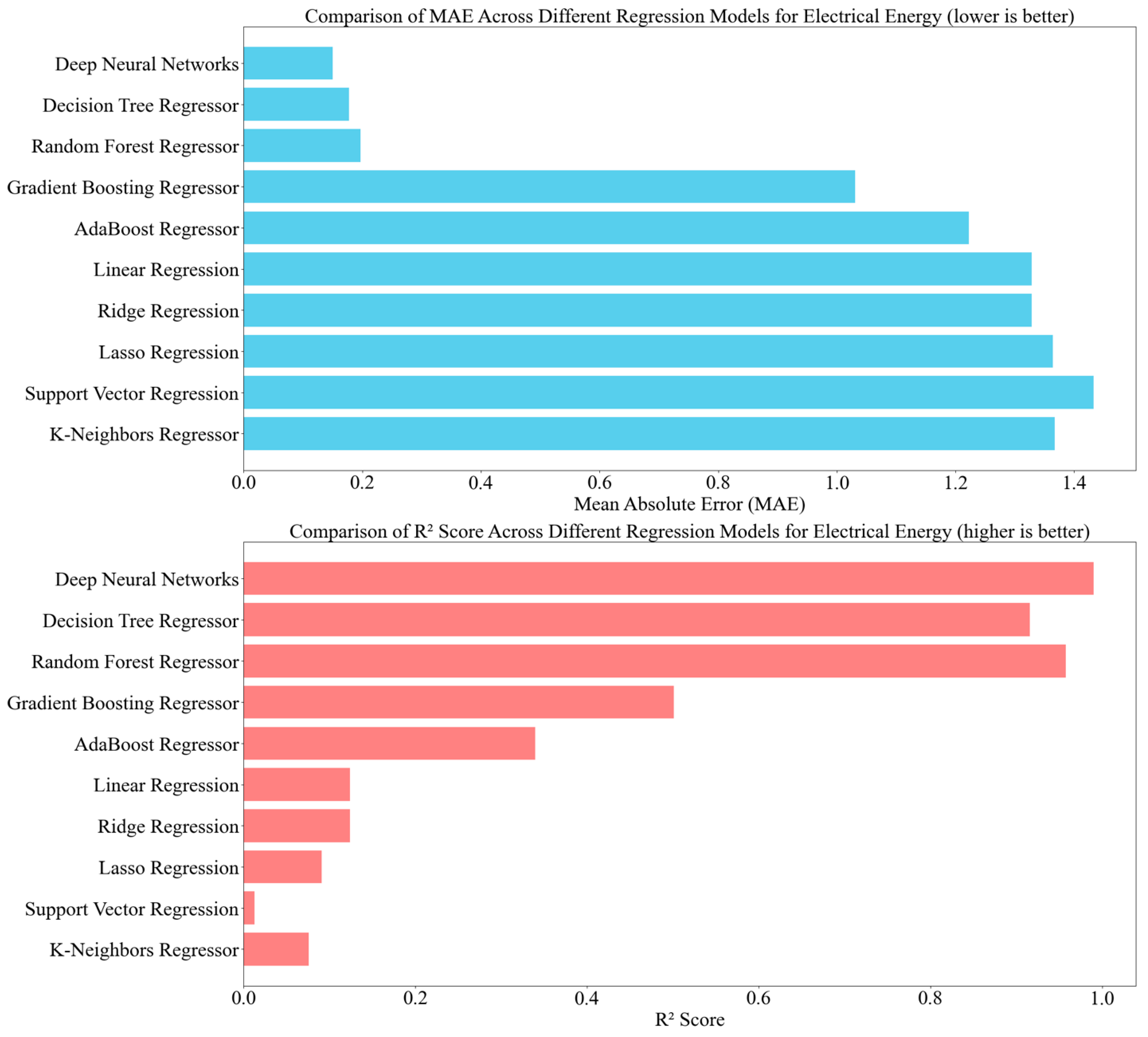
The analysis of various regression models for predicting electrical energy consumption at the UBC Campus, shown in Figure 5, highlighted significant performance differences and emphasized the critical role of model selection in optimizing energy usage. The Deep Neural Networks (DNN) model demonstrated the highest accuracy with a Mean Absolute Error (MAE) of 0.15, and a Coefficient of Determination (R2) of 0.98, indicating its superior capability to capture complex patterns in the data. The Decision Tree Regressor also performed well, achieving an MAE of 0.18 and an R2 of 0.92, reflecting good predictive accuracy. The Random Forest Regressor showed competitive performance with an MAE of 0.20 and an R2 of 0.96, although slightly less accurate than the Decision Tree. In contrast, the Gradient Boosting Regressor had a higher MAE of 1.03 and a lower R2 of 0.50, suggesting less effective prediction capabilities. AdaBoost performed the least effectively, with an MAE of 1.22 and an R2 of 0.34, indicating limited predictive accuracy. Linear Regression, Ridge Regression, Lasso Regression, Support Vector Regression, and K-Neighbors Regressor exhibited poorer performance overall, with MAE values above 1 and lower R2 scores. This analysis underscores the advantage of employing advanced machine learning techniques such as DNNs for accurate energy forecasting, which is crucial for optimizing energy efficiency and resource management at the UBC Campus.
Table 4 provides a clear comparison of the performance metrics of the various regression models, enabling a direct assessment of their effectiveness in predicting electrical energy consumption.

4.3. Hot Water Power

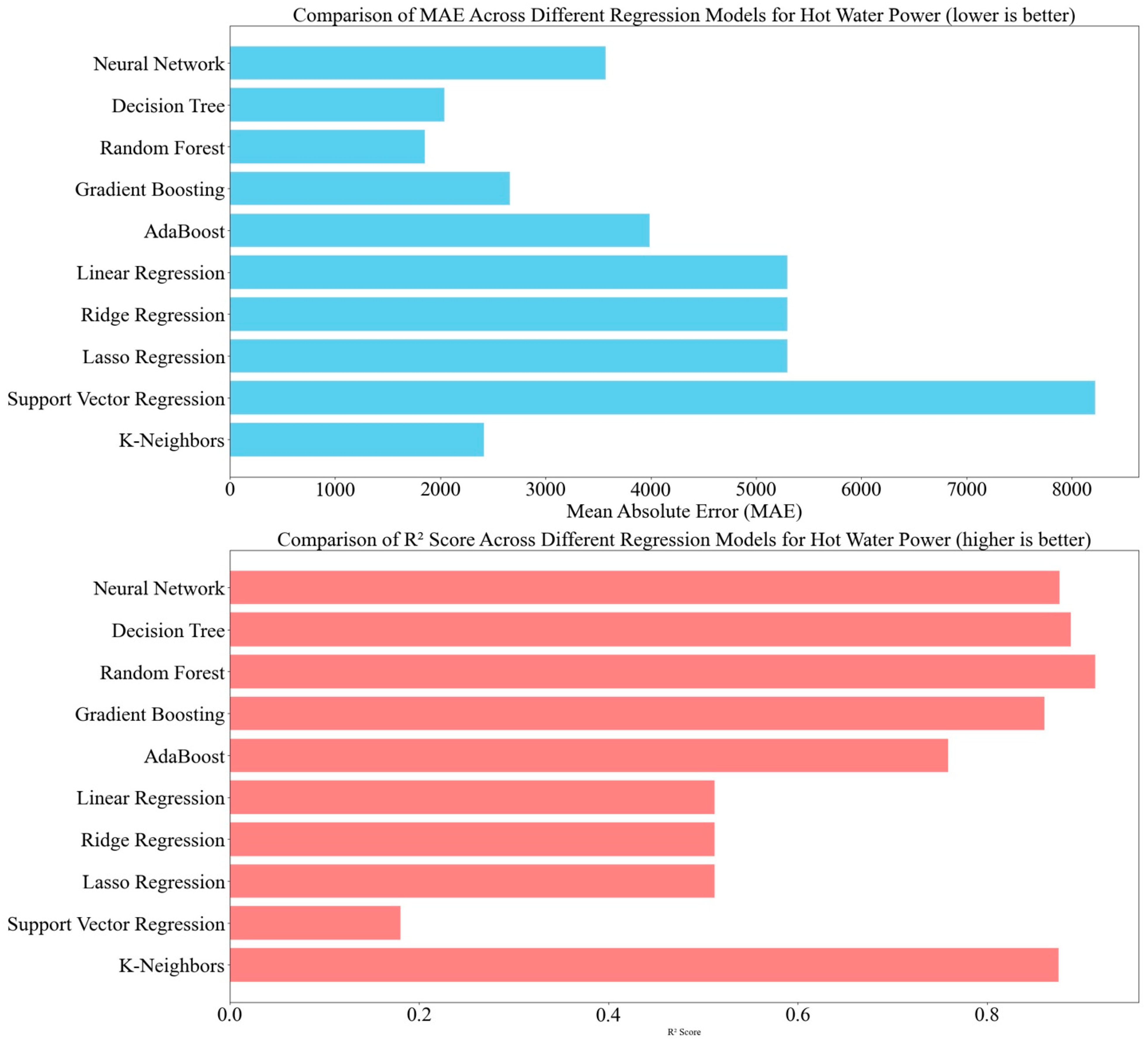
The analysis of various models for predicting hot water power consumption on the UBC campus revealed significant differences in performance (Figure 6). The Neural Network model demonstrated strong predictive performance, with a Mean Absolute Error (MAE) of 3570.00 and a high R2 value of 0.88, indicating its effectiveness in accurately estimating hot water power usage. The Decision Tree Regressor also performed well, with an MAE of 2038.71 and an R2 of 0.89, reflecting its capability to capture patterns and trends in hot water power consumption. The Random Forest Regressor achieved the lowest MAE of 1852.85, and a high R2 value of 0.91, showing its effectiveness in predicting hot water power consumption and managing heating systems efficiently.
In contrast, the Gradient Boosting Regressor had a higher MAE of 2660.06 and a moderate R2, suggesting that further optimization may be required for improved accuracy. AdaBoost Regressor exhibited the highest MAE of 3986.78 and a moderate R2, indicating less effectiveness compared to the top-performing models. The linear models, including Linear Regression, Ridge Regression, and Lasso Regression, had an MAE of around 5298.00 and an R2 of approximately 0.51, providing a baseline with moderate performance but not optimal for precise predictions. Support Vector Regression had the highest MAE of 8222.55 and the lowest R2, indicating significant limitations in accurately modeling hot water power consumption. The KNeighbors Regressor showed reasonable capabilities with an MAE of 2413.37 and an R2 of 0.88, performing comparably to the Neural Network model. Table 5 shows the performance comparison of models for predicting how water power consumption.
In summary, the Neural Network model emerged as the most effective for predicting hot water power consumption, followed closely by the Decision Tree and Random Forest models. These findings underscore the benefits of using advanced machine learning techniques for accurate hot water system management and optimization.

4.4. Gas Volume

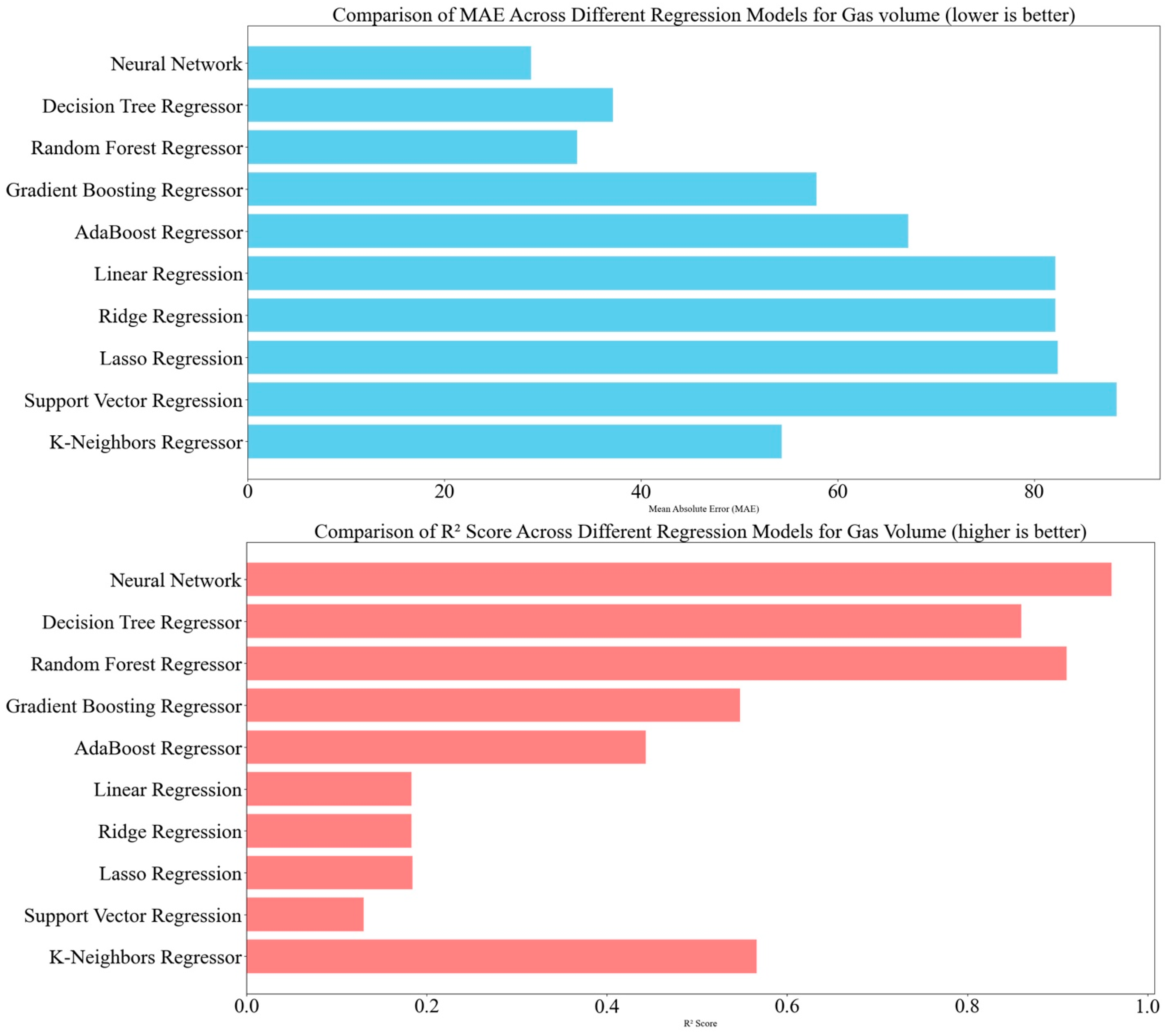
The analysis of various models for predicting gas volume consumption on the UBC campus revealed distinct differences in performance (Figure 7). The Neural Network model emerged as the top performer, achieving a Mean Absolute Error (MAE) of 28.82 and a high R2 value of 0.96. This indicates its exceptional ability to capture the underlying patterns and variability in gas volume data, making it highly effective in optimizing gas usage. The Random Forest Regressor also showed strong performance, with an MAE of 33.51 and an R2 of 0.91, making it a reliable tool for accurate gas volume forecasting. The Decision Tree Regressor demonstrated moderate predictive capabilities with an MAE of 37.17 and an R2 of 0.86. While useful, it may need refinement to achieve the accuracy of the Neural Network and Random Forest models.
In contrast, the Gradient Boosting Regressor exhibited a higher MAE of 57.84 and a moderate R2 of 0.55, indicating some predictive power but also room for improvement. AdaBoost Regressor had the highest MAE of 67.17 and the lowest R2 of 0.44, suggesting limited effectiveness and a need for further optimization. The linear models, including Linear Regression, Ridge Regression, and Lasso Regression, had a poor predictive performance with an MAE of around 82.00 and an R2 of approximately 0.18, providing only a baseline for comparison. Support Vector Regression showed the highest MAE of 88.39 and the lowest R2 of 0.13, reflecting significant limitations in accurately modelling gas volume consumption. The KNeighbors Regressor displayed reasonable performance with an MAE of 54.32 and an R2 of 0.57, performing better than some models but not as effectively as Neural Networks or Random Forest.
The Neural Network model emerged as the most effective for predicting gas volume consumption, with the lowest MAE and highest R2. The Random Forest Regression Model also performed well, and provided accurate forecasts. Other models, such as Decision Trees, Gradient Boosting, AdaBoost, linear regression models, and Support Vector Regression, showed varying degrees of performance, with some needing further refinement to enhance the accuracy. These findings underscore the effectiveness of advanced machine learning techniques for precise gas consumption forecasting and efficient fuel management. Table 6 shows the performance comparison of models for predicting gas volume consumption.

4.5. Synthesis of the Predictive Accuracy for the Different Data Sets

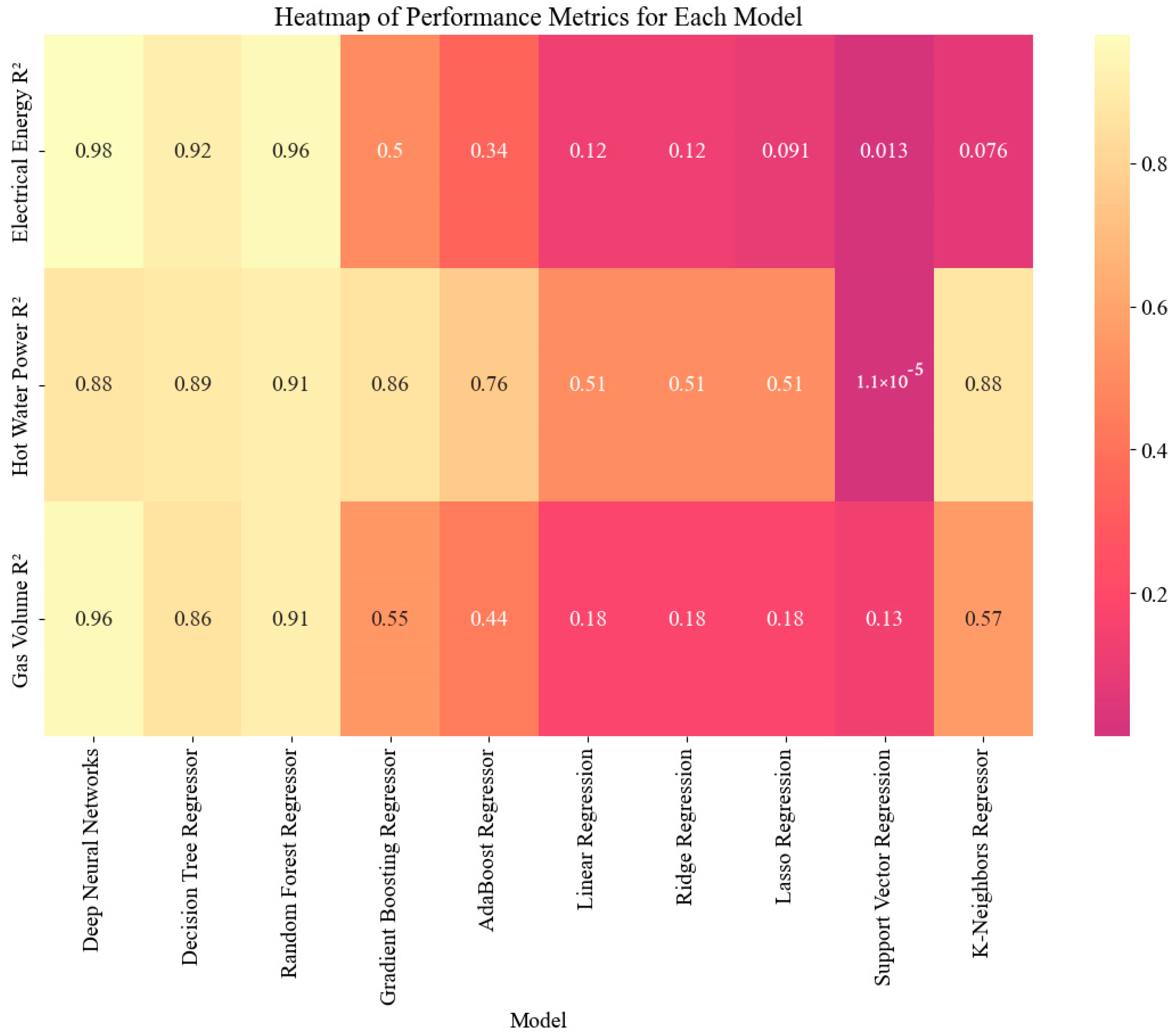
The analysis of the R2 values for various regression models applied to electrical energy, hot water power, and gas volume at the UBC Campus reveals significant differences in the predictive accuracy (Figure 8):
1. Deep Neural Networks consistently demonstrate the highest R2 values across all three energy forms, with an outstanding value of 0.98 for electrical energy, 0.88 for hot water power, and 0.96 for gas volume, indicating solid predictive performance.
2. Decision Tree Regressor and Random Forest Regressor perform well, particularly for hot water power (0.888 and 0.914, respectively) and gas volume (0.863 and 0.914, respectively). However, their performance for electrical energy is somewhat lower (0.916 and 0.958, respectively).
3. Gradient Boosting Regressor and AdaBoost Regressor show moderate performance, with R2 values around 0.50 for electrical energy and gas volume. Still, they perform better for hot water power, with R2 values of 0.860 and 0.759, respectively.
4. Support Vector Regression (SVR) and K-Neighbors Regressor display the least predictive accuracy, with R2 values significantly lower across all energy types, particularly for electrical energy, where the values are 0.013 and 0.076, respectively. These models have limitations in capturing the variability in the data.
5. Simpler models such as Linear Regression, Ridge Regression, and Lasso Regression exhibit notably lower R2 values, particularly for electrical energy, with values approximately 0.124 for both Linear and Ridge Regression and even lower for Lasso Regression at 0.091. Their performance is similarly suboptimal for hot water power and gas volume, where the R2 values hover around 0.512 for both Linear and Ridge Regression, and are slightly lower for Lasso Regression.
Overall, the results indicate that complex models, particularly ensemble methods and deep learning, provide superior predictive accuracy for the energy consumption metrics at the UBC Campus. In contrast, more straightforward regression techniques and some specialized models like SVR and K-Neighbors struggle to effectively capture the data’s variability.

4.6. Analysis of Training and Test Loss Graphs

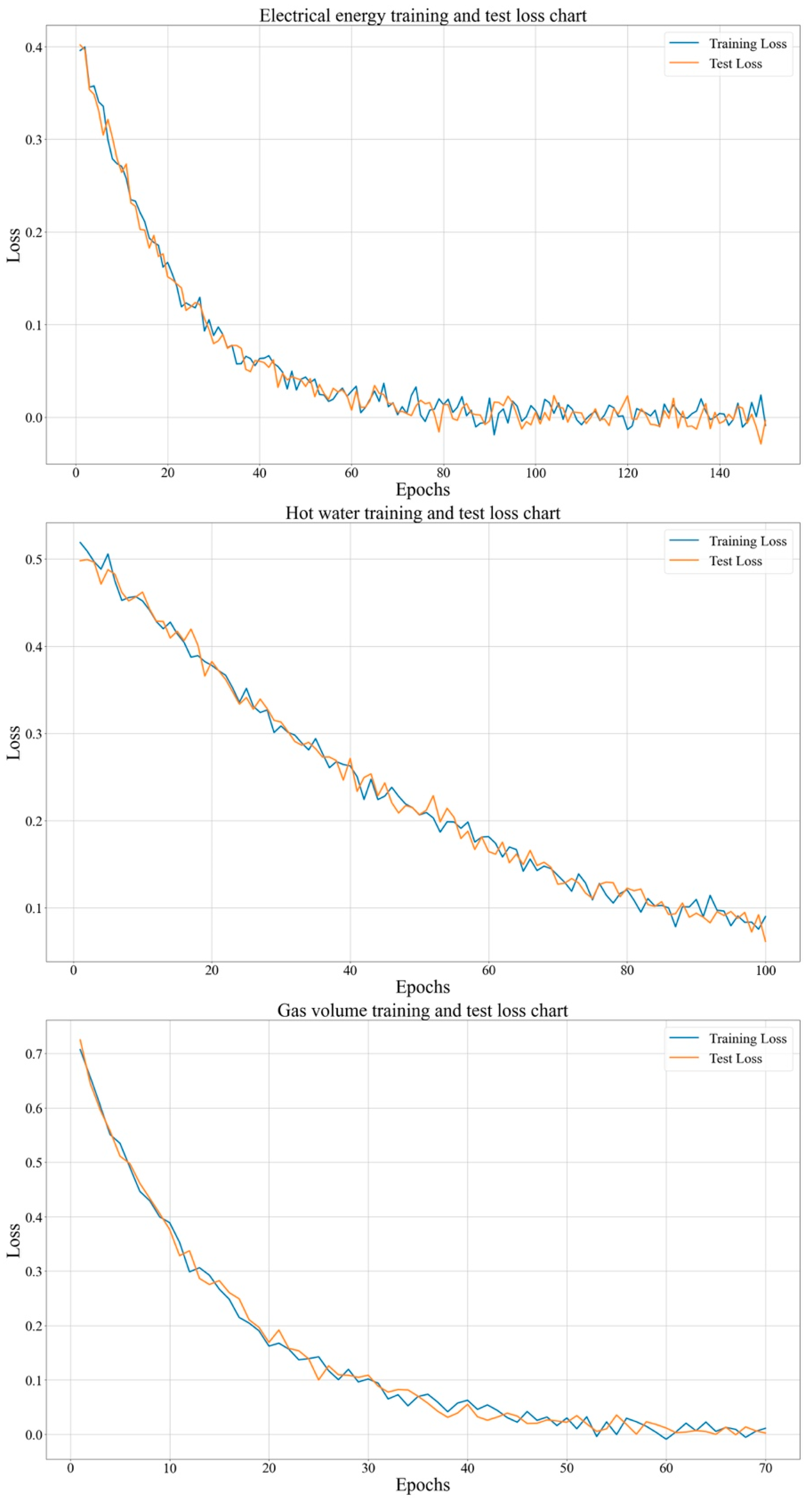
Figure 9 illustrates the training and test loss graphs, showing the different prediction model trends for different energy component data at the UBC Campus. The main observations are as follows:
1.
For the Electrical Energy Model:
Rapid Convergence: This model shows a quick decrease in both training and test losses during the early epochs, indicating effective learning.
Strong Generalization: The close alignment of the training and test loss curves demonstrates that the model generalizes well to unseen data, avoiding overfitting and underfitting.
Balanced Fit: The lack of a significant gap between training and test loss suggests that the model accurately captures the complexity of electrical energy consumption without fitting noise in the data.
2.
Hot Water Model
Slower, Fluctuating Convergence: This model’s loss curves show more fluctuation and a slower decrease, reflecting the challenges in stabilizing it.
Initial Overfitting: Early in training, the model performs better on the training data than on the test data, indicating overfitting.
Improved Generalization: Over time, the gap between the training and test loss narrows, suggesting that the model improves generalization. However, the final model still shows some imbalance.
3.
Gas Volume Model
Gradual Convergence: This model exhibits relatively slow convergence, with a gradual decrease in loss throughout training, suggesting ongoing learning.
Overfitting: The persistent gap between training and test loss indicates that the model may be memorizing training data rather than learning general patterns, pointing to overfitting.
Potential for Improvement: To enhance generalization, the model could benefit from adjustments, such as regularization, more data, or changes in the model architecture.
The strong performance and good generalization of the electrical energy model make it suitable for predicting electrical energy consumption, and we recommend continuing to use this model and monitoring its performance. For the hot water model, it is necessary to address the initial overfitting by applying techniques like early stopping or regularization and ensure that the model maintains balanced performance as it continues to learn. The gas volume model can be improved by exploring regularization methods, expanding the dataset, or adjusting the architecture to better capture patterns and reduce overfitting.
This analysis provides insights into each model’s performance and offers guidance for refining approaches to achieve better predictive accuracy and more effective energy management at the UBC campus.

5. Conclusions

In conclusion, this comprehensive analysis of the energy consumption patterns at the UBC campus in Vancouver has provided critical insights into the intricate relationships among various energy sources, environmental factors, and operational strategies. Through a robust correlation analysis, this study identified significant interdependencies between electricity consumption, hot water power, gas volume, and steam volume, emphasizing the need for an integrated system-wide approach to energy management. Notably, the strong inverse correlations between Vancouver temperature and multiple energy consumption metrics suggest that temperature-responsive strategies could significantly enhance energy efficiency, particularly during warmer periods, aligning with existing research on adaptive energy management practices in temperate climates.
The evaluation of multiple regression models, particularly the superior performance of deep neural networks, highlights their capacity to capture complex, nonlinear patterns in energy consumption data. These models consistently outperformed the traditional methods, demonstrating high predictive accuracy and offering valuable data-driven insights. The effectiveness of these machine learning techniques underscores their potential to optimize energy use, reduce waste, and lower environmental impact, contributing to the growing body of literature that advocates for the application of advanced analytics in energy system optimization.
These findings have substantial implications for energy management in the UBC and similar institutions. By understanding the complex interplay between energy sources, environmental variables, and operational conditions, stakeholders can implement targeted and effective interventions that minimize energy consumption, promote sustainability, and generate cost savings. Furthermore, the success of deep neural networks in this study supports broader theoretical claims regarding the effectiveness of advanced machine learning algorithms in dynamic, multi-source energy systems, aligning with contemporary energy management and artificial intelligence research.
Looking ahead, future research should aim to further elucidate the causal relationships between energy consumption and external factors, evaluate the specific impacts of operational interventions, and explore the potential of integrating renewable energy sources into the campus’s energy portfolio. By building upon the analytical framework and methodologies developed in this study, UBC can continue to lead to sustainable energy management while contributing to a growing body of work focused on reducing institutional environmental footprints and advancing the theoretical understanding of energy optimization.

Author Contributions

Conceptualization, A.S. and A.I.; methodology, A.S.; Coding, A.S.; validation, A.S. and A.I.; formal analysis, A.S.; investigation, A.S.; resources, A.S.; data curation, A.S.; writing—original draft preparation, A.S.; writing—review and editing, A.I.; visualization, A.S.; supervision, A.I.; project administration, A.S. and A.I.; funding acquisition, A.I. All authors have read and agreed to the published version of the manuscript.

Funding

The research was funded by the NSERC Discovery Grant RGPIN-2019-04220, and the APC was funded by MDPI.

Data Availability Statement

The original contributions presented in the study are included in the article and further inquiries can be directed to the corresponding author.

Acknowledgments

This paper’s scientific content is related to the use of multiple AI tools in data analysis. These tools are described extensively in the paper. We did not use generative AI to write the papers. We are systematically using tools to improve editing, i.e., correct grammatical and syntactic errors and improve the vocabulary, as both authors are not native English-speaking. We believe that there are some AI features used in these tools we are using: -Grammarly—(https://app.grammarly.com/ accessed on 13 September 2024)–Antidote—(https://www.antidote.info/en/ accessed on 13 September 2024).

Conflicts of Interest

The authors declare no conflicts of interest.

References

  1. United Nations Environment Programme. 2020 Global Status Report for Buildings and Constructions: Towards a Zero-emission, Efficient and Resilient Buildings and Constructions Sector; United Nations Environmental Programme: Nairobi, Kenya, 2020. [Google Scholar]
  2. Hung, N.T. Data-driven predictive models for daily electricity consumption of academic buildings. Aims Energy 2020, 8, 783–801. [Google Scholar]
  3. Han, B.; Zhang, S.; Qin, L.; Wang, X.; Liu, Y.; Li, Z. Comparison of support vector machine, Gaussian process regression and decision tree models for energy consumption prediction of campus buildings. In Proceedings of the 2022 8th International Conference on Hydraulic and Civil Engineering: Deep Space Intelligent Development and Utilization Forum (ICHCE), Xi’an, China, 25–27 November 2022; IEEE: New York, NY, USA; pp. 689–693. [Google Scholar]
  4. Shahcheraghian, A.; Madani, H.; Ilinca, A. From white to black-box models: A review of simulation tools for building energy management and their application in consulting practices. Energies 2024, 17, 376. [Google Scholar] [CrossRef]
  5. Ding, Y.; Liu, X. A comparative analysis of data-driven methods in building energy benchmarking. Energy Build. 2020, 209, 109711. [Google Scholar] [CrossRef]
  6. Amber, K.P.; Aslam, M.W.; Mahmood, A.; Kousar, A.; Younis, M.Y.; Akbar, B.; Chaudhary, G.Q.; Hussain, S.K. Energy consumption forecasting for university sector buildings. Energies 2017, 10, 1579. [Google Scholar] [CrossRef]
  7. Sadeghian Broujeny, R.; Ben Ayed, S.; Matalah, M. Energy Consumption Forecasting in a University Office by Artificial Intelligence Techniques: An Analysis of the Exogenous Data Effect on the Modeling. Energies 2023, 16, 4065. [Google Scholar] [CrossRef]
  8. Lei, L.; Chen, W.; Wu, B.; Chen, C.; Liu, W. A building energy consumption prediction model based on rough set theory and deep learning algorithms. Energy Build. 2021, 240, 110886. [Google Scholar] [CrossRef]
  9. Fan, C.; Xiao, F.; Zhao, Y. A short-term building cooling load prediction method using deep learning algorithms. Appl. Energy 2017, 195, 222–223. [Google Scholar] [CrossRef]
  10. Chou, J.-S.; Tran, D.-S. Forecasting energy consumption time series using machine learning techniques based on usage patterns of residential householders. Energy 2018, 165, 709–726. [Google Scholar] [CrossRef]
  11. Jarquin, C.S.S.; Gandelli, A.; Grimaccia, F.; Mussetta, M. Short-Term Probabilistic Load Forecasting in University Buildings by Means of Artificial Neural Networks. Forecasting 2023, 5, 390–404. [Google Scholar] [CrossRef]
  12. Gelažanskas, L.; Gamage, K.A. Forecasting hot water consumption in residential houses. Energies 2015, 8, 12702–12717. [Google Scholar] [CrossRef]
  13. Liu, J.; Wang, S.; Wei, N.; Chen, X.; Xie, H.; Wang, J. Natural gas consumption forecasting: A discussion on forecasting history and future challenges. J. Nat. Gas Sci. Eng. 2021, 90, 103930. [Google Scholar] [CrossRef]
  14. UBC. Building Energy and Water Data. Available online: https://energy.ubc.ca/energy-and-water-data/skyspark/ (accessed on 22 April 2024).
  15. UBC. SKy Spark. Available online: https://energy.ubc.ca/projects/skyspark/ (accessed on 22 April 2024).
  16. UBC. University. Building Management Systems (BMS). Available online: https://energy.ubc.ca/ubcs-utility-infrastructure/building-management-systems-bms/ (accessed on 22 April 2024).
  17. UBC. UBC Adress Map. Available online: https://planning.ubc.ca/about-us/campus-maps (accessed on 21 June 2024).
  18. Brownlee, J. How to Decompose Time Series Data into Trend and Seasonality. Available online: https://machinelearningmastery.com/decompose-time-series-data-trend-seasonality/ (accessed on 25 April 2024).
  19. Venujkvenk. Exploring Time Series Data: Unveiling Trends, Seasonality, and Residuals. Available online: https://medium.com/@venujkvenk/exploring-time-series-data-unveiling-trends-seasonality-and-residuals-5cace823aff1 (accessed on 25 April 2024).
  20. Wu, W.; Deng, Q.; Shan, X.; Miao, L.; Wang, R.; Ren, Z. Short-Term Forecasting of Daily Electricity of Different Campus Building Clusters Based on a Combined Forecasting Model. Building 2023, 13, 2721. [Google Scholar] [CrossRef]
  21. Dong, W.; Sun, H.; Li, Z.; Yang, H. Design and optimal scheduling of forecasting-based campus multi-energy complementary energy system. Energy 2024, 309, 133088. [Google Scholar] [CrossRef]
  22. UBC. Hot Water District Energy System. Available online: https://energy.ubc.ca/ubcs-utility-infrastructure/district-energy-hot-water/ (accessed on 12 July 2024).
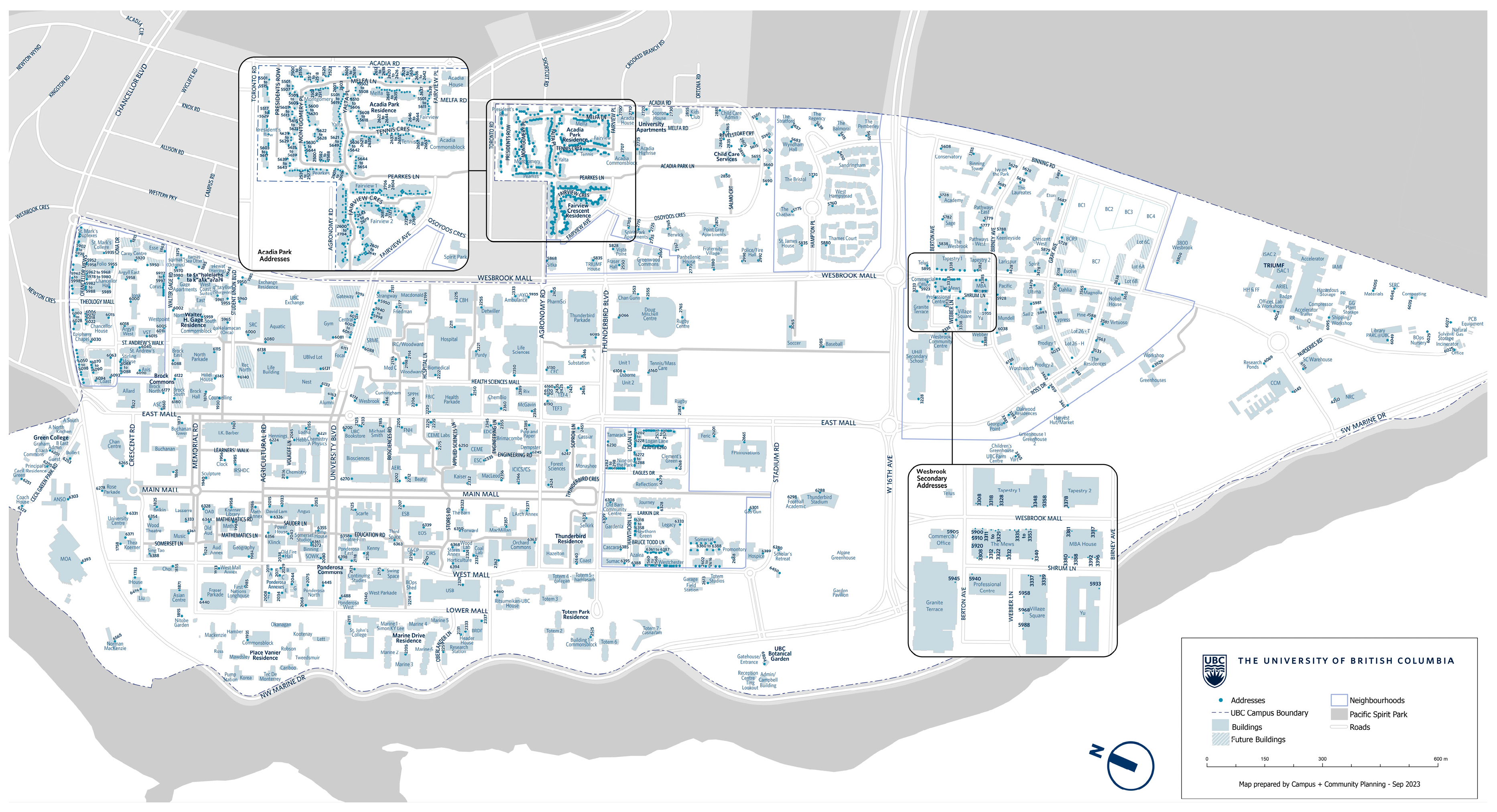
Figure 1. UBC campus building map [17].
Energies 17 04714 g001
Figure 2. Total electricity energy and total hot water power of the UBC Campus in 2023.
Energies 17 04714 g002
Figure 3. Seasonal decomposition of total electrical energy for 2023.
Energies 17 04714 g003
Figure 4. Correlation matrix for weather and energy in UBC Campus.
Energies 17 04714 g004
Figure 5. Comparison of MAE and R2 Scores for electricity energy.
Energies 17 04714 g005
Figure 6. Comparison of MAE and R2 scores for hot water power.
Energies 17 04714 g006
Figure 7. Comparison of MAE and R2 scores for gas volume.
Energies 17 04714 g007
Figure 8. Heatmap of R2 squared.
Energies 17 04714 g008
Figure 9. Training and test loss trends for energy usage prediction models at UBC Vancouver Campus.
Energies 17 04714 g009
Table 1. HyperParameters for the ML models.
ModelBest Parameters
Decision Tree Regressor{‘max_depth’: 20, ‘min_samples_split’: 5, ‘min_samples_leaf’: 2, ‘max_features’: ‘sqrt’}
Random Forest Regressor{‘n_estimators’: 100, ‘max_depth’: 20, ‘min_samples_split’: 2, ‘min_samples_leaf’: 4, ‘max_features’: ‘auto’}
Gradient Boosting Regressor{‘n_estimators’: 100, ‘learning_rate’: 0.1, ‘max_depth’: 5, ‘subsample’: 0.9}
AdaBoost Regressor{‘n_estimators’: 100, ‘learning_rate’: 0.1, ‘loss’: ‘linear’}
Linear Regression{‘fit_intercept’: True, ‘normalize’: False}
Ridge Regression{‘alpha’: 1.0, ‘solver’: ‘auto’}
Lasso Regression{‘alpha’: 0.1, ‘selection’: ‘cyclic’}
Support Vector Regression{‘C’: 1.0, ‘epsilon’: 0.1, ‘kernel’: ‘rbf’, ‘degree’: 3}
K-Neighbors Regressor{‘n_neighbors’: 5, ‘weights’: ‘uniform’, ‘p’: 2, ‘algorithm’: ‘auto’}
Table 2. Hyperparameters of the ANN model.
CategoryHyperparameterValue/Description
Layer StructureFirst LayerDense layer with 128 neurons, ‘tanh’ activation function
Second LayerDense layer with 64 neurons, ‘tanh’ activation function
Third LayerDense layer with 64 neurons, ‘tanh’ activation function
Fourth LayerDense layer with 32 neurons, ‘tanh’ activation function
Output LayerDense layer with 1 neuron for regression output
Activation FunctionActivation Function‘tanh’ (used in all hidden layers)
The ‘tanh’ activation function was chosen for its ability to introduce nonlinearity into the model, which is crucial for capturing complex patterns in energy consumption data. It outputs values between −1 and 1, centering the data and helping to address the vanishing gradient problem. Additionally, ‘tanh’ handles negative inputs effectively, which aligns with the characteristics of our dataset. This choice helps improve the model’s learning dynamics and performance.
RegularizationDropout Rate0.4 (applied after each BatchNormalization layer)
Kernel RegularizerL2 regularization with factor 0.01 (applied to the weights of the second, third, and fourth Dense layers)
OptimizationOptimizerNadam
Learning Rate0.0005
Learning Rate SchedulerReduceLROnPlateau (reduces learning rate by 0.5 if validation loss does not improve for 10 epochs, minimum learning rate set to 1 × 10⁻⁶)
Training ConfigurationBatch Size16
Epochs100
CallbacksCustom CallbackTestLossCallback (tracks test loss at the end of each epoch)
Table 3. Correlation analysis of energy consumption metrics and environmental factors at UBC Campus.
Metric PairCorrelationInterpretation
Electricity Energy and Hot Water Power0.38 (Moderate Positive)Increases in electricity usage are moderately associated with increases in hot water power consumption.
Electricity Energy and Gas Volume0.25 (Weaker Positive)Weaker positive relationship; changes in electricity usage have a less pronounced effect on gas volume.
Electricity Energy and Steam Volume0.31 (Moderate Positive)Moderate positive correlation; notable relationship between electricity usage and steam volume.
Hot Water Power and Steam Volume0.75 (Strong Positive)Strong positive correlation and significant relationship due to UBC’s medium-temperature hot water system.
Hot Water Power and Gas Volume0.34 (Moderate Positive)Moderate positive relationship between hot water power consumption and gas volume.
Gas Volume and Steam Volume0.49 (Moderate Positive)Moderate positive correlation; considerable relationship between gas and steam volumes.
Seasonal Effects and Temperature0.19 (Weak Positive)Weak positive correlation; mild influence of seasonal variations on temperature fluctuations.
Temperature and Hot Water Power−0.69 (Strong Negative)Strong negative correlation; warmer temperatures are associated with reduced hot water power usage.
Temperature and Steam Volume−0.60 (Strong Negative)Strong negative correlation; warmer temperatures are associated with reduced steam volume.
Temperature and Electricity Energy−0.27 (Moderate Negative)Moderate negative correlation; warmer temperatures are associated with a noticeable reduction in electricity use.
Table 4. Performance comparison of regression models for predicting electrical energy consumption.
ModelMean Absolute Error (MAE)Coefficient of Determination (R2)
Deep Neural Networks (DNN)0.150.98
Decision Tree Regressor0.180.92
Random Forest Regressor0.20.96
Gradient Boosting Regressor1.030.5
AdaBoost Regressor1.220.34
Linear Regression>1Lower values
Ridge Regression>1Lower values
Lasso Regression>1Lower values
Support Vector Regression>1Lower values
K-Neighbors Regressor>1Lower values
Table 5. Performance comparison of models for predicting hot water power consumption.
ModelMAER2
Neural Network35700.88
Decision Tree Regressor2038.710.89
Random Forest Regressor1852.850.91
Gradient Boosting Regressor2660.06Moderate
AdaBoost Regressor3986.78Moderate
Linear Regression~5298.00~0.51
Ridge Regression~5298.00~0.51
Lasso Regression~5298.00~0.51
Support Vector Regression8222.55Lowest
KNeighbors Regressor2413.370.88
Table 6. Performance comparison of models for predicting gas volume consumption.
ModelMAER2
Neural Network28.820.96
Random Forest Regressor33.510.91
Decision Tree Regressor37.170.86
Gradient Boosting Regressor57.840.55
AdaBoost Regressor67.170.44
Linear Regression~82.00~0.18
Ridge Regression~82.00~0.18
Lasso Regression~82.00~0.18
Support Vector Regression88.390.13
KNeighbors Regressor54.320.57
Disclaimer/Publisher’s Note: The statements, opinions and data contained in all publications are solely those of the individual author(s) and contributor(s) and not of MDPI and/or the editor(s). MDPI and/or the editor(s) disclaim responsibility for any injury to people or property resulting from any ideas, methods, instructions or products referred to in the content.