A Hybrid Approach for Hierarchical Forecasting of Industrial Electricity Consumption in Brazil

Abstract

The Brazilian industrial sector is the largest electricity consumer in the power system. Energy planning in this sector is important mainly due to its economic, social, and environmental impact. In this context, electricity consumption analysis and projections are highly relevant for the decision-making of the industrial sectorand organizations operating in the energy system. The electricity consumption data from the Brazilian industrial sector can be organized into a hierarchical structure composed of each geographic region (South, Southeast, Midwest, Northeast, and North) and their respective states. This work proposes a hybrid approach that incorporates the projections obtained by the exponential smoothing and Box–Jenkins models to obtain the hierarchical forecasting of electricity consumption in the Brazilian industrial sector. The proposed approach was compared with the bottom-up, top-down, and optimal combination approaches, which are widely used for time series hierarchical forecasting. The performance of the models was evaluated using the mean absolute percentage error (MAPE) and root mean squared error (RMSE) precision measures. The results indicate that the proposed hybrid approach can contribute to the projection and analysis of industrial sector electricity consumption in Brazil.

1. Introduction

The electricity consumption in the Brazilian industrial sector has been investigated over the last few years, mainly due to its importance in economic, environmental, and social terms, in addition to being one of the main indicators of a country’s development. Thus, the analysis and projections of electricity consumption are extremely relevant information for planning the electricity system and also for the development of the industrial sector in Brazil.

In Brazil, electricity consumption in the industrial sector varies between states, since consumption depends on public policies and the type of industrial activity that changes from state to state. In addition, consumption can be organized in a hierarchical structure, considering the hierarchy defined for Brazil as the top level, with the geographic regions (North, Northeast, Midwest, Southeast and South) as the intermediate level and the states of the federation as a lower level. This structure has as its fundamental characteristic the grouping of time series at lower levels to form a series at another level of the hierarchy. Recently, bottom-up, top-down and optimal combination approaches have been used to forecast hierarchical time series of electricity consumption [1,2,3].

In the bottom-up approach, forecasts are achieved for the time series that occupy the lowest level of the hierarchy and are aggregated to form predictions at the higher levels. A very high level of detail is required in the hierarchy structure, but this is necessary to prevent any loss of information due to grouping. However, the top-down approach generates forecasts of the aggregated series and, in some situations, disaggregates such forecasts based on historical proportions to the required levels. Finally, the optimal combination approach performs forecasting of each series of all levels of the hierarchy separately and, after this, combines the forecasts through a regression model.

This work proposes a hybrid approach that combines bottom-up and top-down methods using Monte Carlo simulation for electricity consumption forecasting in the Brazilian industrial sector. This proposal was compared to bottom-up, top-down and optimal combination approaches. To implement these approaches, time series models of Box–Jenkins and exponential smoothing were considered. These predictive models can capture trend components, changes in level and seasonality of the industrial sector’s electricity consumption time series.

The paper is organized as follows. Section 2 presents a review of relevant works in the literature on hierarchical forecasting of energy consumption, while Section 3 presents a theoretical description of the time series models and the hierarchical forecasting approaches. Section 4 presents a description of the data and the results. Finally, Section 5 provides the main conclusions and some possibilities for future research.

2. Literature Review

The bottom-up approach has been used in energy systems modeling since 1980 [4]. Herbst et al. [5] evaluated future energy demand and supply using bottom-up and top-down energy models. The authors pointed out that a bottom-up model has greater data detail when compared to a top-down model. Dunn et al. [6] showed that bottom-up forecasts are more accurate than those obtained by the top-down approach due to data detailing.

The bottom-up, top-down and optimal reconciliation approaches have been investigated in different research areas for hierarchical forecasting. Hyndman et al. [7] proposed an optimal combination approach for hierarchical forecasting that provides better forecasts than the bottom-up and top-down approaches. Athanasopoulos et al. [8] compared these three approaches through hierarchical forecasting results. Hyndman et al. [9] presented the least squares method to reconcile hierarchical time series forecasts. Wickramasuriya et al. [10] employed the optimal combination method, incorporating information from a covariance matrix through forecast errors. Wickramasuriya et al. [11] developed a methodology for hierarchical time series reconciliation that is constrained to provide non-negative forecasts. These studies were applied to Australian domestic tourism data. Spinelli et al. [12] presented a hierarchical control structure to optimize the operation of a Smart Thermal Energy Grid. Lila et al. [13] introduced the robust estimation concept for hierarchical forecast reconciliation methods using unemployment data in Brazil. Wang et al. [14] presented a review of the available hierarchical forecasting combination methods.

Fleiter et al. [15] presented a deterministic bottom-up approach to obtain long-term electricity consumption forecasts for the German pulp and paper industry. Reyna and Chester [16] used a bottom-up approach to forecast the residential electricity consumption in Los Angeles County (California). This study explored the potential for energy efficiency. Huang et al. [17] used the same approach to obtain the long-term electricity projection of the cement industry in Taiwan. Ben Taieb et al. [1] adopted a hierarchical probabilistic forecasting method for energy supply data in a power grid in Great Britain. Besagni et al. [18] adopted a bottom-up model applied to the Italian residential sector. Wang et al. [19] developed a bottom-up approach for short-term residential sector load forecasting using publicly available datasets from the Netherlands and Canada. Nespoli et al. [20] showed a comparison between different forecasters of electrical demand using data from an urban distribution network in Switzerland. Spiliotis et al. [3] proposed a modification of the Multiple Aggregation Prediction Algorithm (MTA) for high-frequency time series. MTA and the optimal reconciliation method were integrated, presenting good hierarchical forecasting performance for electricity consumption data. Brégère and Huard [21] presented a three-step approach to hierarchical forecasting electricity consumption time series at different levels of household sector aggregation using data from Great Britain.

In Brazil, Silva et al. [22] introduced a bottom-up approach to obtain long-term electricity consumption forecasting in the pulp and paper industry. Silva et al. [2] proposed a model that integrates hierarchical linear models with a bottom-up approach, applied to the electricity consumption in the Brazilian pulp and paper industry. Silva et al. [23] presented a comparative study using artificial neural network models for electricity consumption forecasting in the Brazilian industrial sector. Meira et al. [24] presented a hierarchical forecasting reconciliation approach to provide accurate forecasts for energy demand at all levels of an energy system. This study used electric energy consumption data from the Brazilian National Interlinked System (SIN). Vellasco et al. [25] presented a hierarchical neuro-fuzzy model for hourly electric load forecasting of Brazilian electric power companies.

Recently, machine learning algorithms have been used for electricity hierarchical forecasting. Mancuso et al. [26] proposed a machine learning approach for forecasting hierarchical time series, employing a deep neural network to extract information capturing the hierarchy structure. Pang et al. [27] developed the hierarchical forecast of electricity consumption using multiple alternative clustering methods. Shaikh et al. [28] developed a method of Neural Basis Expansion Analysis for interpretable Time Series (N-BEATS). This method was applied to energy consumption data in London Households. Yang et al. [29] introduced an iterative decompose-cluster-feedback algorithm to improve the forecasts at the total level of the hierarchy structure. Carpinteiro et al. [30] presented a hierarchical hybrid neural model for long-term load forecasting.

This section presented a literature review of different works on forecasting hierarchical time series. The hybrid approach proposed in this work has not been developed in any research. In addition, this study showed a comparison analysis between the main hierarchical forecasting approaches. The advantage of this proposed methodology is that the time series models are adjusted to electricity consumption for each Brazilian state and combined with the result of the model fitted for Brazil as a whole. The main disadvantage is the data detailing necessary for the preprocessing of the hierarchical structure presented in this work. In the literature review, some studies also require a data volume similar to that of the approach proposed here.

3. Methodology

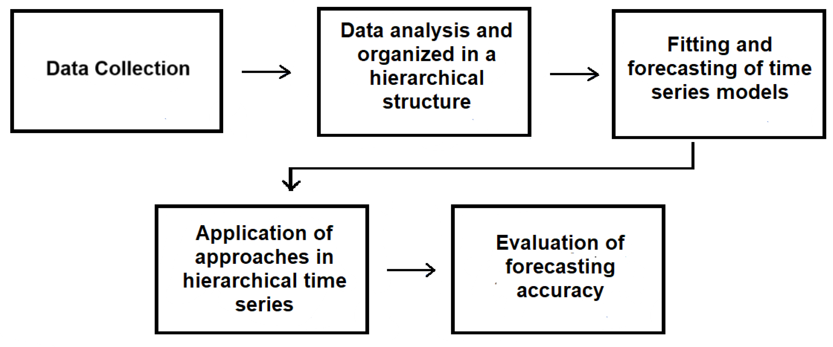
This section presents the steps of the methodology, a theoretical description of time series models, and the hierarchical forecasting approaches. The methodology steps are presented in the flowchart (Figure 1).

In the first stage, monthly data on electricity consumption (GWh) of the industrial sector were obtained, from January 2004 to December 2021, available on the website of the Energy Research Company (EPE) [31]. Brazil is a country composed of five regions: North (N), Northeast (NT), Midwest (MW), Southeast (ST) and South (S). Each region contains a certain amount of states, with a total of 27 states. In this step, data preprocessing was performed following the hierarchical structure levels (Brazil, regions and states). The data were organized so that they could be used by the approaches adopted in this work.

The North region contains the states of Acre (AC), Amapá (AP), Amazonas (AM), Pará (PA), Roraima (RR), Rondônia (RO) and Tocantins (TO). The Northeast region contains the states of Alagoas (AL), Bahia (BA), Ceará (CE), Maranhão (MA), Rio Grande do Norte (RN), Sergipe (SE), Paraíba (PB), Pernambuco (PE) and Piauí (PI). The Midwest region contains the states of Mato Grosso (MT), Mato Grosso do Sul (MS), Goiás (GO) and Distrito Federal (DF). In the Southeast region, São Paulo (SP), Minas Gerais (MG), Rio de Janeiro (RJ) and Espírito Santo (ES). Finally, in the South region, the states are Paraná (PR), Santa Catarina (SC) and Rio Grande do Sul (RS).

Each state stands out in a specific industrial activity. For example, Pará stands out in the mining industry, the states of Bahia, Goiás and Rio Grande do Sul stand out in the construction sector, while Rio de Janeiro stands out for its oil and gas industry. Thus, each state has different seasonality cycles and trends, since industrial electricity consumption is influenced by industrial activity and public policies. In the second stage of the methodology, the data were organized in a hierarchical structure of two levels, considering the electricity consumption by geographic regions and states of the federation, including the Federal District. See the hierarchy illustration in Figure 2.

Then, the time series classical models of exponential smoothing and Box–Jenkins were fitted to the data and provided predictions. In the next step, bottom-up, top-down, hybrid, and optimal blending hierarchical time series approaches incorporated energy consumption forecasts provided by exponential smoothing and Box–Jenkins models. Finally, in the last step, the forecasting accuracy of the approaches was evaluated using the mean absolute percentage error (MAPE) and the root mean squared error (RMSE) in different training and test sets. This assessment is important to determine the effectiveness of the model in predicting future values based on available historical data.

To assess the forecasting accuracy of the approaches, the hierarchical time series were divided into two sets: the training set, to adjust and validate the models, and the test set, used to assess their accuracy. Thus, five scenarios of training and testing sets were proposed. In the first scenario, the training set considered the observations from January 2004 to December 2016. The test set is always defined as twelve observations ahead of the training set, from January 2017 to December 2017. In the second scenario, the training set was augmented with twelve observations from 2017, the test set with data from January 2018 to December 2018, and so on until the fifth and final scenario. Finally, the MAPE and RMSE accuracy measures were calculated for each scenario and the average was taken by approach to compare the bottom-up, top-down, hybrid, and optimal combination methods.

All analyses and development of hierarchical approaches were performed using the Statistical Software R 4.4.0 [32].

3.1. Hierarchical Time Series

Time series that are organized in a hierarchical structure and can be aggregated at different levels of the hierarchy are called hierarchical time series. The electricity consumption data in the Brazilian industrial sector can be disaggregated by geographical region (five regions) and by state (27 states), thus characterizing a hierarchical structure with two levels and a total of 33 series. The mathematical notation presented in this work follows the development of Hyndman et al. [7] and Athanasopoulos et al. [8]. For each month t, let $Y_{B,t}$ be Brazil’s electricity consumption, $Y_{Regions,t}$ represents the stacked vector of all five regions, $Y_{states,t}$ is the stacked vector of all $m=27$ states and, the vector ${\mathbf{Y}}_t={[Y_{B,t},Y_{Regions,t},Y_{states,t}]}^{\prime }$ of dimension $n=33$. The aggregated time series can be represented by the following matrix equation

$${\mathbf{Y}}_t=S_{(n\times m)}{Y}_{states,t},$$

(1)

where S is a summation matrix of order $n\times m$, such that $n=33$ is the total number of series in the data and $m=27$ is the number of series at the base of the hierarchy. In turn, the summation matrix is written in the form

$$S_{(n\times m)}=\left[\begin{array}{ccccccccccccccccccccccccccc}1& 1& 1& 1& 1& 1& 1& 1& 1& 1& 1& 1& 1& 1& 1& 1& 1& 1& 1& 1& 1& 1& 1& 1& 1& 1& 1\\ 1& 1& 1& 1& 1& 1& 1& 0& 0& 0& 0& 0& 0& 0& 0& 0& 0& 0& 0& 0& 0& 0& 0& 0& 0& 0& 0\\ 0& 0& 0& 0& 0& 0& 0& 1& 1& 1& 1& 1& 1& 1& 1& 1& 0& 0& 0& 0& 0& 0& 0& 0& 0& 0& 0\\ 0& 0& 0& 0& 0& 0& 0& 0& 0& 0& 0& 0& 0& 0& 0& 0& 1& 1& 1& 1& 0& 0& 0& 0& 0& 0& 0\\ 0& 0& 0& 0& 0& 0& 0& 0& 0& 0& 0& 0& 0& 0& 0& 0& 0& 0& 0& 0& 1& 1& 1& 1& 0& 0& 0\\ 0& 0& 0& 0& 0& 0& 0& 0& 0& 0& 0& 0& 0& 0& 0& 0& 0& 0& 0& 0& 0& 0& 0& 0& 1& 1& 1\\ & & & & & & & & & & & & & I_m& & & & & & & & & & & & \end{array}\right]$$

where $I_m$ denotes the $m\times m$ identity matrix with $m=27$. The values of one in the matrix S indicate the existence of states, while zeros do not, to generate the aggregated electricity consumption for Brazil and by region. Thus, the first row of this matrix represents Brazil as a country composed of twenty-seven states; the second row represents the North region composed of seven corresponding states; the third row, the Northeast region composed of nine corresponding states; the fourth row, the Midwest region composed of three corresponding states and the Federal District; the fifth row, the Southeast region composed of four states; and, finally, the sixth row, the South region composed of three states. The rows of the identity matrix $I_m$ characterize each corresponding state in order to allow the construction of aggregated time series.

In order to obtain the forecast equation, ${\tilde{Y}}_{T+h}$ denotes a set of combined forecasts h steps ahead. Thus, the forecasting matrix equation is given by

$${\tilde{Y}}_{T+h}=SG{\widehat{Y}}_{T+h},$$

(2)

where ${\widehat{Y}}_{T+h}$ are the base forecasts, which are independent forecasts of all series in the hierarchy, and G is a matrix referring to the type of hierarchical forecasting approach adopted.

3.1.1. Bottom-Up Approach

This approach consists of using predictive models for each series at the lower level and then grouping them to produce forecasts for the entire hierarchical structure. An advantage inherent in this approach is that by predicting at the lower levels of the hierarchy, there is no loss of information through grouping. The bottom-up approach can be represented using the matrix G constructed by

$$G=\left[0_{m\times (n-m)}\right|I_m],$$

(3)

in which $I_m$ is the identity matrix of order m and $0_{m\times (n-m)}$ is the zero matrix of order $m\times (n-m)$.

3.1.2. Top-Down Approach

In the top-down approach, the forecast for the top-level time series of the hierarchy is obtained first and then disaggregated to the lower levels using a set of proportions $\mathbf{p}={(p_1,p_2,\cdots ,p_m)}^{\prime }$, where m is the number of series at the base of the hierarchy. These proportions dictate how the forecast should be distributed among the lower-level series. Generally, for a fixed set of proportions, the top-down approach can be represented by

$${\tilde{Y}}_{T+h}=SG{\widehat{Y}}_{T+h}$$

(4)

where the matrix G is constructed such that

$$G=\left[\mathbf{p}\right|0_{m\times (n-1)}].$$

(5)

The first column includes the proportions set that distributes the base forecasts from the top level to the lower level. The remaining columns nullify the base forecasts below the highest level of aggregation. This work is not interested in disaggregating the time series forecasting of the upper level to the series of the lower level.

3.1.3. Optimal Combination Approach

This approach performs independent forecasting of all time series of the hierarchical structure and then uses a regression model to combine and reconcile these forecasts optimally. This method aims to find a matrix G that minimizes the prediction error of the combined set of predictions [7].

Firstly, the combined forecasts should be obtained using the Equation (2). If the forecasts at the base of the hierarchy are unbiased, then the predictions for the rest of the hierarchy will also be impartial as long as $SGS=S$. Thus, we have a restriction for constructing the matrix G. According to Wickramasuriya et al. [10], the variance–covariance matrix of the forecast errors h steps ahead is given by

$$V_h=Var[Y_{T+h}-{\tilde{Y}}_{T+h}]=SG{W}_h{G}^{\prime }{S}^{\prime }$$

(6)

where $W_h=Var[Y_{T+h}-{\widehat{Y}}_{T+h}]$ is the variance–covariance matrix of the forecast errors at the base level of the hierarchy. Therefore, the objective is to find the matrix G that minimizes the variances of the combined forecasts. Since the variances are on the diagonal of $V_h$, the sum of all variances is equal to the trace of $V_h$. Thus, the matrix G that minimizes the trace of $V_h$ is given by

$$G={\left(S^{\prime }{W}_h^{-1}S\right)}^{-1}{S}^{\prime }{W}_h^{-1}$$

(7)

Therefore, by substituting Equation (7) into the equation ${\tilde{Y}}_{T+h}=SG{\widehat{Y}}_{T+h}$, we have that

$${\tilde{Y}}_{T+h}=S{\left(S^{\prime }{W}_h^{-1}S\right)}^{-1}{S}^{\prime }{W}_h^{-1}{\widehat{Y}}_{T+h}$$

(8)

In the optimal combination method, the optimal matrix G depends only on the matrix S, i.e., the method depends on the hierarchical organization. For more details on the calculation of the matrix $W_h$, see Hyndman et al. [9].

3.1.4. Hybrid Approach

The main contribution of this paper is the proposal of a hybrid approach between the bottom-up and top-down approaches. Suppose a hierarchical structure where the series at the first level and the series at the lowest level have T observations each, constituting the training sets. In this procedure, one-step-ahead predictions are obtained independently by the bottom-up approach for the series at the lowest level and aggregated, ${\widehat{Y}}_{T+1}^{bottom}$, and by the top-down approach for the series at the first level, ${\widehat{Y}}_{T+1}^{top}$. Thus, the distribution of the prediction, ${\widehat{Y}}_{T+1}^{hybrid}$, obtained by the hybrid approach is considered to be normal and it is given by

$${\widehat{Y}}_{T+1}^{hybrid}\sim \mathcal{N}ORMAL({\widehat{\mu }}_{T+1},{\widehat{\sigma }}_{T+1}^2)$$

(9)

where the mean of the distribution, ${\widehat{\mu }}_{T+1}$, is an arithmetic mean between the two projections, through bottom-up and top-down approaches, and the variance, ${\widehat{\sigma }}_{T+1}^2$, is the quadratic deviance between these projections, ensuring that the hybrid forecast remains within the range bounded by these forecasts:

$${\widehat{\mu }}_{T+1}=\frac{{\widehat{Y}}_{T+1}^{bottom}+{\widehat{Y}}_{T+1}^{top}}{2}\mathrm{and}{\widehat{\sigma }}_{T+1}^2={\left(\frac{\left|{\widehat{Y}}_{T+1}^{bottom}-{\widehat{Y}}_{T+1}^{top}\right|}{2}\right)}^2.$$

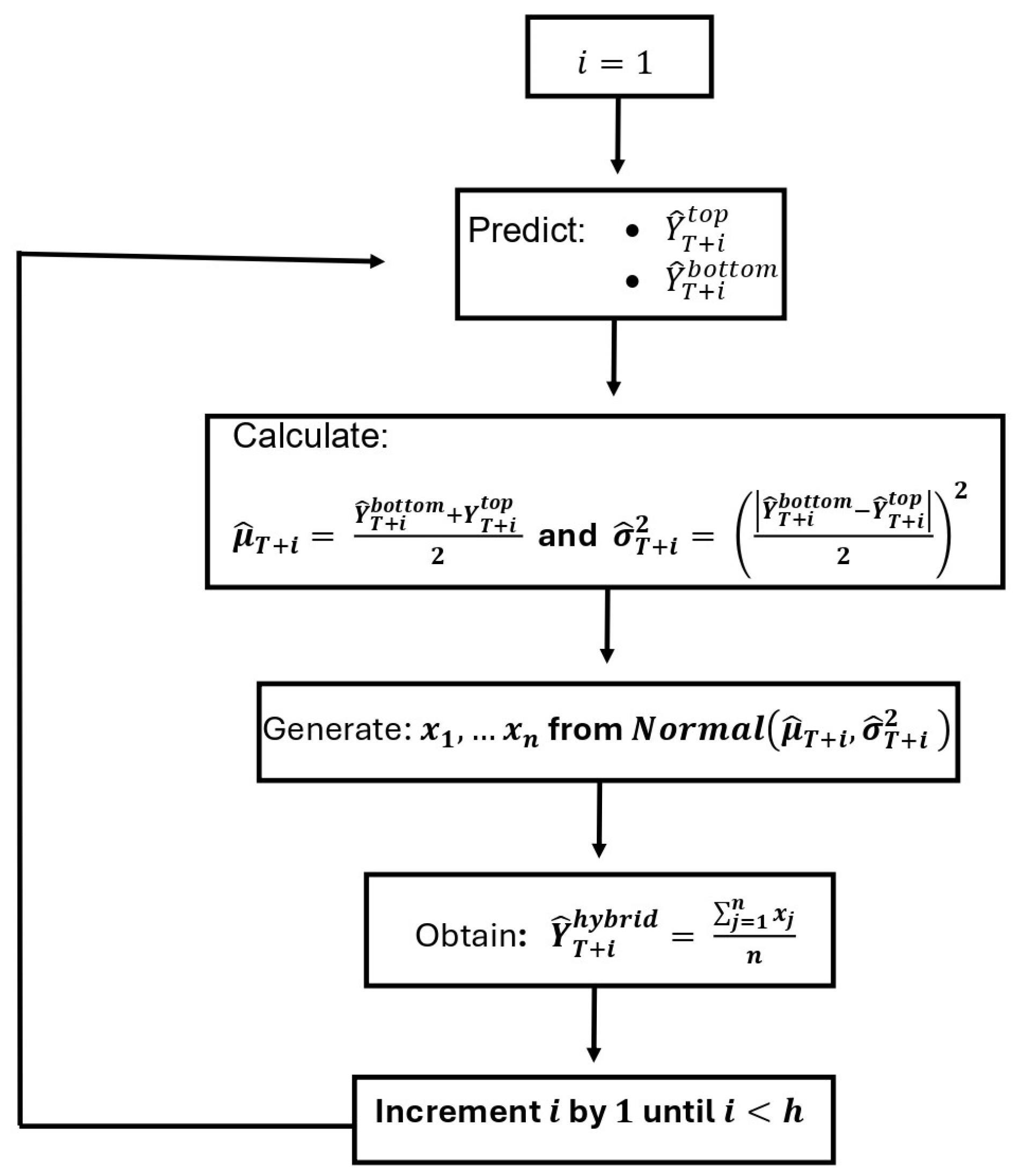
Using the Monte Carlo simulation method, it is possible to generate samples of ${\widehat{Y}}_{T+1}^{hybrid}$ for each time in the forecast horizon. The algorithm to implement this method can be described in a summarized way as follows:

• Step 1: Prediction for the Brazil series.
• Step 2: Forecasting each series in the base and aggregating for higher levels up to the fully aggregated series.
• Step 3: Create a vector containing the average ${\widehat{\mu }}_{T+1}$ between each forecast top-down and bottom-up obtained in step 1 and step 2.
• Step 4: Create a vector containing the variance ${\widehat{\sigma }}_{T+1}^2$ between each forecast top-down and bottom-up obtained in the step 1 and step 2.
• Step 5: Generate a sample of size n from a normal distribution with mean ${\widehat{\mu }}_{T+1}$ and variance ${\widehat{\sigma }}_{T+1}^2$ at each time T.
• Step 6: Create a prediction vector of the hybrid approach containing the mean of each sample obtained in step 5 in the temporal order.

Therefore, to generate forecasts h steps ahead, it is sufficient to repeat the process described above, as shown by the flowchart of the proposed algorithm in Figure 3.

3.2. Time Series Models

Hierarchical forecasting approaches rely on time series forecasts at the lower level of the hierarchy structure. Thus, the projections are obtained by time series models and incorporated into the hierarchical approaches. In this work, the exponential smoothing and Box–Jenkins models were used, which are widely used in the time series forecasting literature.

The exponential smoothing model was proposed in the 1950s by [33,34,35]. In this method, forecasts are derived through a weighted average of past observations, with observation weights decreasing exponentially as the observations age. The structure of the exponential smoothing model is constructed by identifying the error, trend and seasonality components (additive or multiplicative) present in time series [36,37]. The choice of the exponential smoothing models was carried out by the ETS (Error, Trend and Seasonality) algorithm proposed by Hyndman et al. [38,39,40].

The Box–Jenkins methodology is widely used in the parametric time series model analysis [41]. This methodology consists of fitting autoregressive integrated moving average (ARIMA) models to a data set using the autocorrelation functions between observations. The Box–Jenkins model was obtained through the algorithm proposed by Hyndman and Khandakar [39].

3.3. Forecasting Accuracy Measures

In order to compare all the models, the forecasting accuracy measures MAPE and RMSE were used. Let N be the number of predicted values, ${\widehat{Y}}_i$ is the forecast value, and $Y_i$ is the observed value for time i. The model comparison metrics are defined as follows

$$MAPE=100\times \frac{1}{N}\sum _{i=1}^N\left|\frac{Y_i-\widehat{Y_i}}{Y_i}\right|$$

(10)

$$RMSE=\sqrt{\frac{1}{N}\sum _{i=1}^N{(Y_i-{\widehat{Y}}_i)}^2}.$$

(11)

4. Application

4.1. Data Description

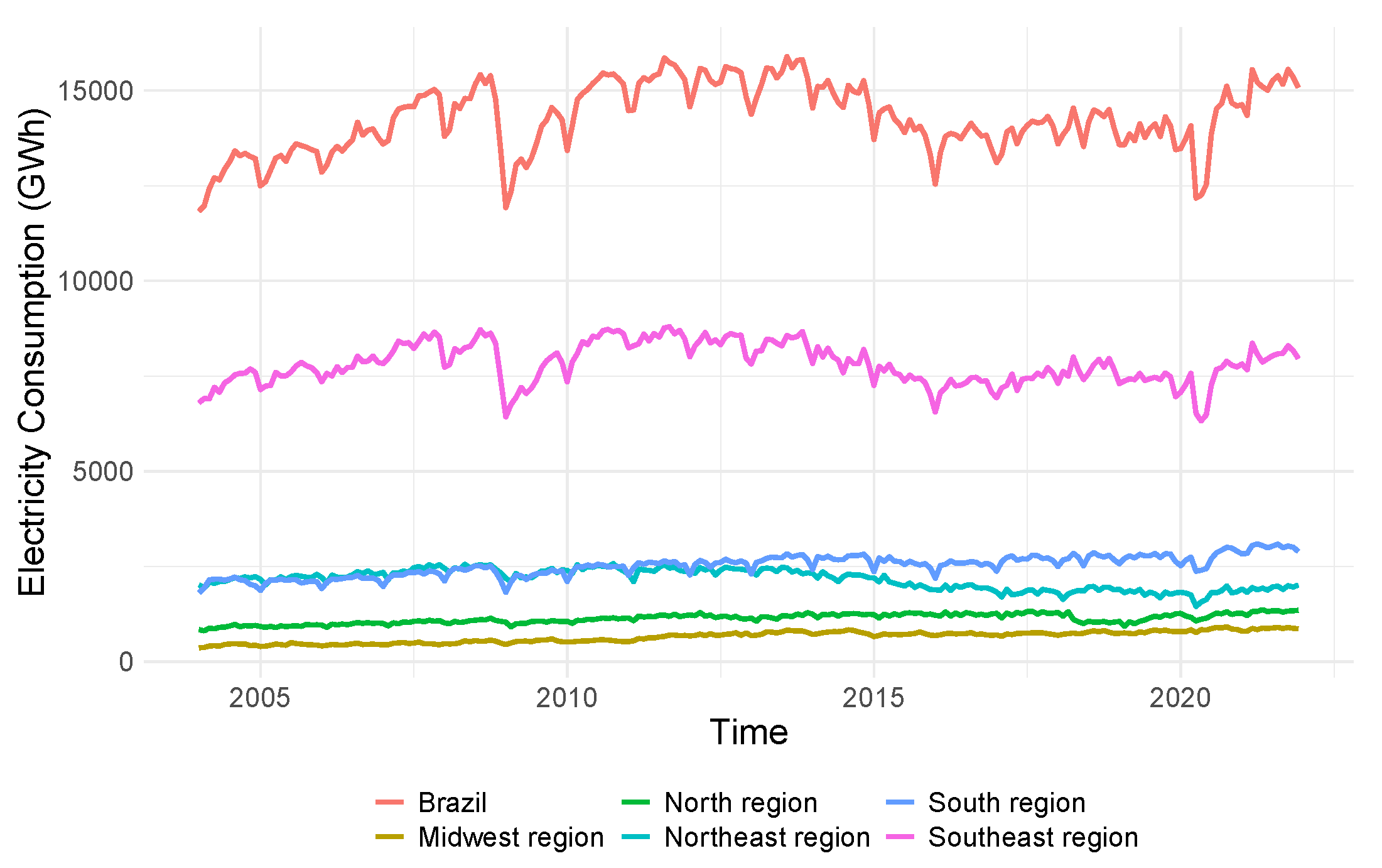
The electricity consumption data of the Brazilian industrial sector can be divided by geographical regions, which in turn can be divided by states, forming a hierarchical structure. Figure 4 shows the trajectory of electricity consumption in the Brazilian industrial sector and the geographical regions. This figure shows that the electricity consumption time series in the Southeast region has a trajectory similar to that of Brazil, indicating the region’s importance in the energy system. The energy consumption time series in the Northeast region shows a damped downward trend. The Midwest region has the lowest electricity consumption in its industrial sector. Electricity consumption in the Southern region has been growing over the years and occupies the second position in quantity consumed in 2021 (Figure 4).

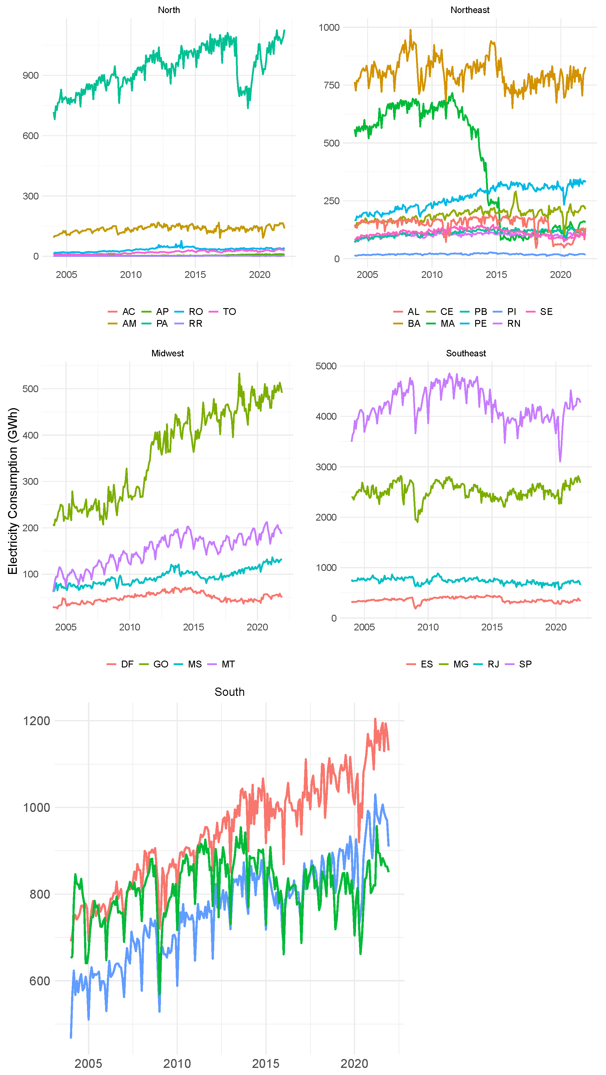
The electricity consumption in the industrial sector of Brazilian states can be observed in Figure 5. The industrial sector electricity consumption of the Pará state is the highest in the North region. There is a decline in the industrial sector electricity consumption for the Maranhão state in the Northeast region starting from 2011. The Bahia state has the highest electricity consumption, while Piauí has the lowest. It can be observed that the industrial sector in the Federal District showed a decline in electricity consumption, which is different from the rest of the states in the Midwest region. The state of São Paulo has the highest electricity consumption of the Brazilian industrial sector. For the states in the South region, there is an increase in electricity consumption over time.

4.2. Results and Discussion

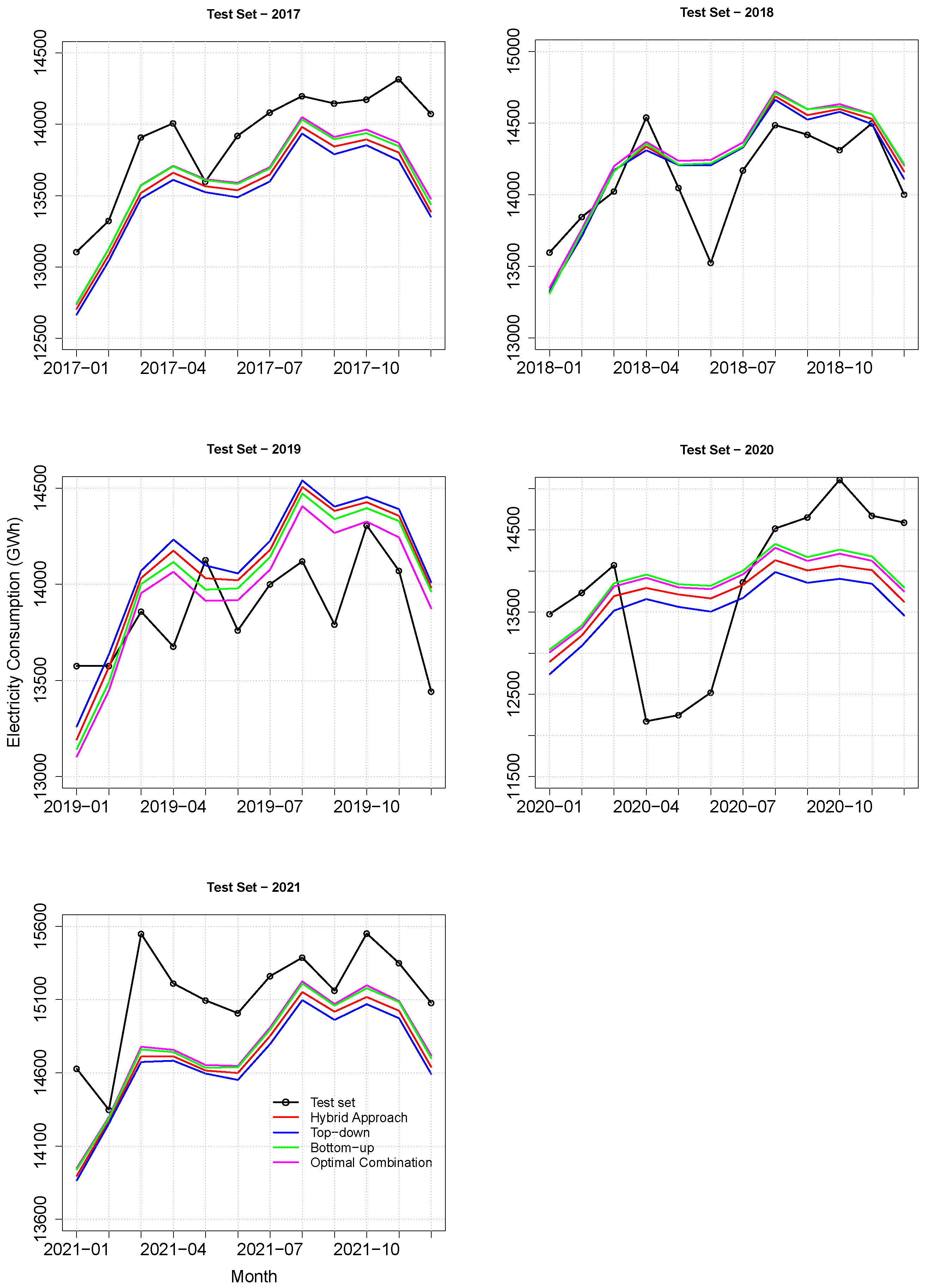
This section presents the results obtained by the bottom-up, top-down, hybrid and optimal combination approaches applied to the electricity consumption data of the Brazilian industrial sector. Figure 6 shows a comparison between the forecasts via the four approaches using an exponential smoothing model for all test sets. The model projections captured the series-level changes in all test sets. The forecasts for 2017 and 2021 were slightly underestimated, which did not happen in 2019.

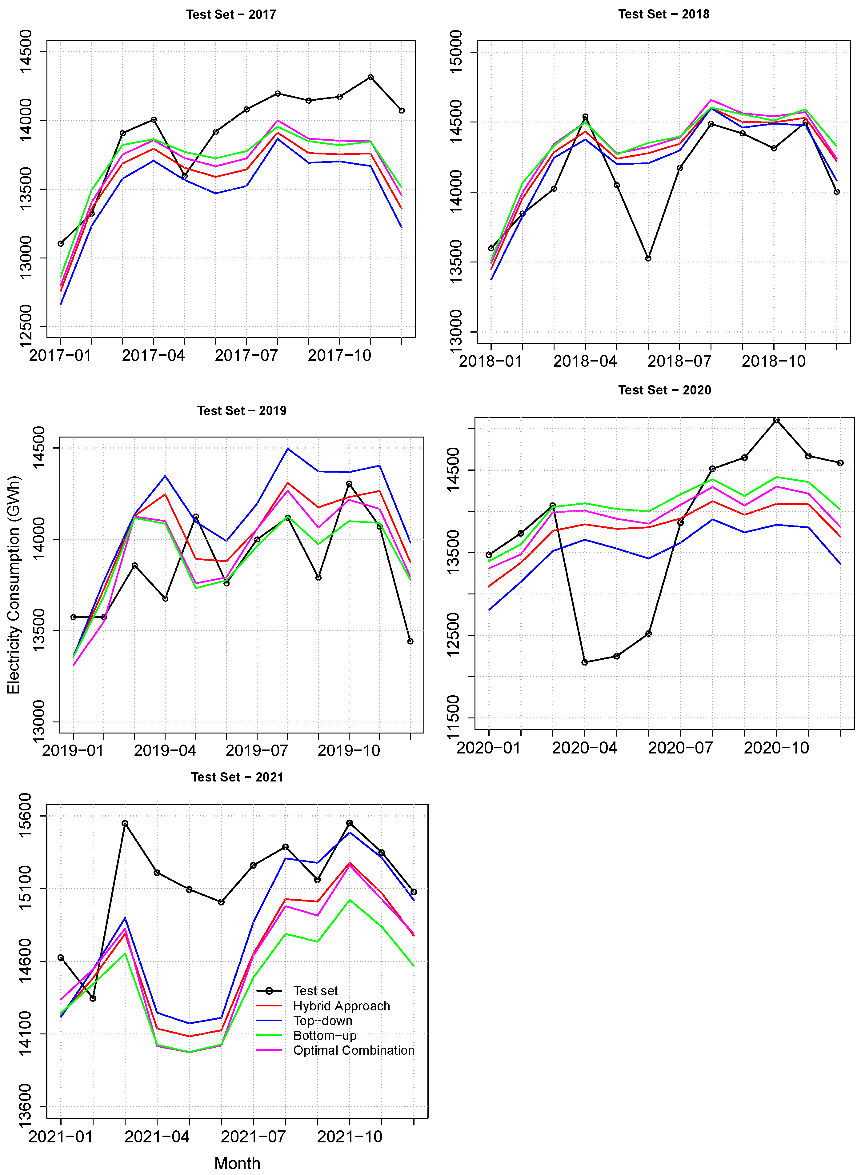
The forecasts obtained through the Box–Jenkins model integrated into the approaches for all test sets are presented in Figure 7. In 2017, the forecasts for the initial months were close to the test set and for the remaining months, there was an underestimation. For the test sets of 2018, 2019, and 2020, the predictions captured most of the behavior in the data. There was a deviation from the forecast for the initial months of 2021 and, on the other hand, the model presented better forecasts for the last months of 2021.

Table 1. Forecasting performance of the approaches for the Brazilian industrial sector electricity consumption data using exponential smoothing model.

Test Set	2017		2018		2019
	MAPE	RMSE	MAPE	RMSE	MAPE	RMSE
Bottom-up	2.70%	409.76	2.09%	357.25	1.67%	310.59
	2020		2021		Average
	MAPE	RMSE	MAPE	RMSE	MAPE	RMSE
	5.74%	924.35	2.47%	428.05	2.93%	486.00
Test set	2017		2018		2019
	MAPE	RMSE	MAPE	RMSE	MAPE	RMSE
Top-Down	2.85%	426.19	1.46%	258.89	2.27%	364.55
	2020		2021		Average
	MAPE	RMSE	MAPE	RMSE	MAPE	RMSE
	6.39%	936.34	3.03%	503.98	3.20%	497.59
Test set	2017		2018		2019
	MAPE	RMSE	MAPE	RMSE	MAPE	RMSE
Optimal *	2.61%	396.51	2.08%	352.20	1.55%	296.43
	2020		2021		Average
	MAPE	RMSE	MAPE	RMSE	MAPE	RMSE
	5.83%	926.81	2.38%	415.29	2.89%	477.45
Test set	2017		2018		2019
	MAPE	RMSE	MAPE	RMSE	MAPE	RMSE
Hybrid **	2.51%	382.44	1.54%	266.41	2.12%	341.14
	2020		2021		Average
	MAPE	RMSE	MAPE	RMSE	MAPE	RMSE
	5.81%	898.13	2.76%	467.87	2.95%	471.20

* Optimal combination approach described in Section 3. ** Hybrid approach described in Section 3.

and

Table 2. Forecasting performance of the approaches for the Brazilian industrial sector electricity consumption data using Box and Jenkins model.

Test Set	2017		2018		2019
	MAPE	RMSE	MAPE	RMSE	MAPE	RMSE
Bottom-up	2.24%	357.16	2.38%	381.05	1.37%	246.25
	2020		2021		Average
	MAPE	RMSE	MAPE	RMSE	MAPE	RMSE
	5.35%	941.24	4.38%	736.14	3.14%	532.37
Test set	2017		2018		2019
	MAPE	RMSE	MAPE	RMSE	MAPE	RMSE
Top-Down	2.95%	465.64	1.21%	238.10	2.25%	364.73
	2020		2021		Average
	MAPE	RMSE	MAPE	RMSE	MAPE	RMSE
	6.51%	954.62	2.58%	518.13	3.10%	508.24
Test set	2017		2018		2019
	MAPE	RMSE	MAPE	RMSE	MAPE	RMSE
Optimal *	2.35%	371.95	2.22%	359.29	1.22%	241.11
	2020		2021		Average
	MAPE	RMSE	MAPE	RMSE	MAPE	RMSE
	5.58%	929.87	3.67%	656.90	3.01%	511.82
Test set	2017		2018		2019
	MAPE	RMSE	MAPE	RMSE	MAPE	RMSE
Hybrid **	2.37%	377.89	1.42%	265.51	1.70%	273.24
	2020		2021		Average
	MAPE	RMSE	MAPE	RMSE	MAPE	RMSE
	5.68%	901.91	3.39%	611.04	2.91%	485.92

* Optimal combination approach described in Section 3. ** Hybrid approach described in Section 3.

present the comparison between the forecasting performance of the approaches in each of the five sets of the test set. Both tables show MAPE and RMSE measure values for each test set and the average value among the tested periods. In Table 1, the hybrid approach via the exponential smoothing model presented the lowest value for the average RMSE, meaning it had the best forecasting performance compared to the other approaches. On the other hand, the lowest average value in terms of MAPE was obtained by the optimal combination method. Additionally, the approaches presented average MAPE values between the test sets below $4\%$.

In Table 2, the values of the MAPE and RMSE measures of the approaches were obtained by incorporating the predictions obtained via the Box–Jenkins models. The hybrid approach presented the lowest MAPE and RMSE average, indicating better forecasting accuracy.

5. Conclusions

This work considered a hierarchical structure for electricity consumption in the Brazilian industrial sector, with Brazil at the top level, geographic regions at the intermediate level, and states at the bottom level. From this hierarchical structure, a hybrid approach is proposed combining the forecasts via top-down and bottom-up approaches, in order to forecast the electricity consumption of the Brazilian industrial sector. The predictive models of exponential smoothing and Box–Jenkins were integrated into each of the bottom-up, top-down, optimal combination, and hybrid approaches to make predictions. The performance of these approaches was compared using different test sets through the MAPE and RMSE comparison metrics.

The results showed the approaches integrated with predictive models had an average MAPE below $4\%$. Based on the MAPE, the proposed hybrid approach presented the best forecasting accuracy using the Box–Jenkins model. On the other hand, the optimal combination approach provided the best forecasting performance using the exponential smoothing model. From the RMSE, the proposed hybrid approach demonstrated the best forecasting performance through the exponential smoothing and Box-Jenkins models.

The approaches combined with the predictive models were able to capture the structure of the data involving the economic crises (2009 and 2016) and the COVID-19 pandemic. In addition, the results found are useful as decision-support tools and can contribute to energy planning in the industrial sector in Brazil. An interesting issue for future work would be to integrate the predictive models of neural networks with the approaches used in this study. Likewise, this approach could be extended to other scenarios, such as those addressed in [42,43,44,45]. Another interesting work would be to evaluate the effect of energy efficiency policies, taking into account the hierarchical structure (Brazil, regions, and states). Finally, another avenue for future work would be to consider the Brazilian industry segments in the hierarchical structure.

References

- Ben Taieb, S.; Taylor, J.; Hyndman, R. Hierarchical Probabilistic Forecasting of Electricity Demand With Smart Meter Data. J. Am. Stat. Assoc. 2020, 116, 1–36. [Google Scholar] [CrossRef]
- da Silva, F.L.; Cyrino Oliveira, F.L.; Souza, R.C. A bottom-up bayesian extension for long term electricity consumption forecasting. Energy 2019, 167, 198–210. [Google Scholar] [CrossRef]
- Spiliotis, E.; Petropoulos, F.; Kourentzes, N.; Assimakopoulos, V. Cross-temporal aggregation: Improving the forecast accuracy of hierarchical electricity consumption. Appl. Energy 2020, 261, 114339. [Google Scholar] [CrossRef]
- Chateau, B.; Lapillonne, B. Long-term energy demand forecasting A new approach. Energy Policy 1978, 6, 140–157. [Google Scholar] [CrossRef]
- Herbst, A.; Toro, F.; Reitze, F. Introduction to Energy Systems Modelling. Swiss J. Econ. Stat. 2012, 148, 111–135. [Google Scholar] [CrossRef]
- Dunn, D.; Williams, W.; Dechaine, T. Aggregate Versus Subaggregate Models in Local Area Forecasting. J. Am. Stat. Assoc. 1976, 71, 68–71. [Google Scholar] [CrossRef]
- Hyndman, R.J.; Ahmed, R.A.; Athanasopoulos, G.; Shang, H.L. Optimal combination forecasts for hierarchical time series. Comput. Stat. Data Anal. 2011, 55, 2579–2589. [Google Scholar] [CrossRef]
- Athanasopoulos, G.; Ahmed, R.A.; Hyndman, R.J. Hierarchical forecasts for Australian domestic tourism. Int. J. Forecast. 2009, 25, 146–166. [Google Scholar] [CrossRef]
- Hyndman, R.J.; Lee, A.J.; Wang, E. Fast computation of reconciled forecasts for hierarchical and grouped time series. Comput. Stat. Data Anal. 2016, 97, 16–32. [Google Scholar] [CrossRef]
- Wickramasuriya, S.L.; Athanasopoulos, G.; Hyndman, R.J. Optimal Forecast Reconciliation for Hierarchical and Grouped Time Series Through Trace Minimization. J. Am. Stat. Assoc. 2019, 114, 804–819. [Google Scholar] [CrossRef]
- Wickramasuriya, S.L.; Turlach, B.A.; Hyndman, R.J. Optimal non-negative forecast reconciliation. Stat. Comput. 2020, 30, 1167–1182. [Google Scholar] [CrossRef]
- Spinelli, S.; Farina, M.; Ballarino, A. An optimal hierarchical control scheme for smart generation units: An application to combined steam and electricity generation. J. Process. Control 2020, 94, 58–74. [Google Scholar] [CrossRef]
- Lila, M.F.; Meira, E.; Cyrino Oliveira, F.L. Forecasting unemployment in Brazil: A robust reconciliation approach using hierarchical data. Socio-Econ. Plan. Sci. 2022, 82, 101298. [Google Scholar] [CrossRef]
- Wang, X.; Hyndman, R.J.; Li, F.; Kang, Y. Forecast combinations: An over 50-year review. Int. J. Forecast. 2022, 30, 1518–1547. [Google Scholar] [CrossRef]
- Fleiter, T.; Fehrenbach, D.; Worrell, E.; Eichhammer, W. Energy efficiency in the German pulp and paper industry—A model-based assessment of saving potentials. Energy 2012, 40, 84–99. [Google Scholar] [CrossRef]
- Reyna, J.; Chester, M. Energy efficiency to reduce residential electricity and natural gas use under climate change. Nat. Commun. 2017, 8, 14916. [Google Scholar] [CrossRef] [PubMed]
- Huang, Y.H.; Chang, Y.L.; Fleiter, T. A critical analysis of energy efficiency improvement potentials in Taiwan’s cement industry. Energy Policy 2016, 96, 14–26. [Google Scholar] [CrossRef]
- Besagni, G.; Borgarello, M.; Premoli Vilà, L.; Najafi, B.; Rinaldi, F. MOIRAE—Bottom-up MOdel to compute the energy consumption of the Italian REsidential sector: Model design, validation and evaluation of electrification pathways. Energy 2020, 211, 118674. [Google Scholar] [CrossRef]
- Wang, S.; Deng, X.; Chen, H.; Shi, Q.; Xu, D. A bottom-up short-term residential load forecasting approach based on appliance characteristic analysis and multi-task learning. Electr. Power Syst. Res. 2021, 196, 107233. [Google Scholar] [CrossRef]
- Nespoli, L.; Medici, V.; Lopatichki, K.; Sossan, F. Hierarchical demand forecasting benchmark for the distribution grid. Electr. Power Syst. Res. 2020, 189, 106755. [Google Scholar] [CrossRef]
- Brégère, M.; Huard, M. Online hierarchical forecasting for power consumption data. Int. J. Forecast. 2022, 38, 339–351. [Google Scholar] [CrossRef]
- Silva, F.L.; Souza, R.C.; Cyrino Oliveira, F.L.; Lourenco, P.M.; Calili, R.F. A bottom-up methodology for long term electricity consumption forecasting of an industrial sector—Application to pulp and paper sector in Brazil. Energy 2018, 144, 1107–1118. [Google Scholar] [CrossRef]
- Silva, F.; da Costa, K.; Rodrigues, P.; Salas, R.; Linkolk, J. Statistical and Artificial Neural Networks Models for Electricity Consumption Forecasting in the Brazilian Industrial Sector. Energies 2022, 15, 588. [Google Scholar] [CrossRef]
- Meira, E.; Lila, M.F.; Cyrino Oliveira, F.L. A novel reconciliation approach for hierarchical electricity consumption forecasting based on resistant regression. Energy 2023, 269, 126794. [Google Scholar] [CrossRef]
- Vellasco, M.M.B.; Pacheco, M.A.C.; Neto, L.S.R.; de Souza, F.J. Electric load forecasting: Evaluating the novel hierarchical neuro-fuzzy BSP model. Int. J. Electr. Power Energy Syst. 2004, 26, 131–142. [Google Scholar] [CrossRef]
- Mancuso, P.; Piccialli, V.; Sudoso, A.M. A machine learning approach for forecasting hierarchical time series. Expert Syst. Appl. 2021, 182, 115102. [Google Scholar] [CrossRef]
- Pang, Y.; Zhou, X.; Zhang, J.; Sun, Q.; Zheng, J. Hierarchical electricity time series prediction with cluster analysis and sparse penalty. Pattern Recognit. 2022, 126, 108555. [Google Scholar] [CrossRef]
- Shaikh, A.K.; Nazir, A.; Khan, I.; Shah, A.S. Short term energy consumption forecasting using neural basis expansion analysis for interpretable time series. Sci. Rep. 2022, 12, 22562. [Google Scholar] [CrossRef] [PubMed]
- Yang, Y.; Zhou, H.; Wu, J.; Liu, C.J.; Wang, Y.G. A novel decompose-cluster-feedback algorithm for load forecasting with hierarchical structure. Int. J. Electr. Power Energy Syst. 2022, 142, 108249. [Google Scholar] [CrossRef]
- Carpinteiro, O.A.; Leme, R.C.; de Souza, A.C.Z.; Pinheiro, C.A.; Moreira, E.M. Long-term load forecasting via a hierarchical neural model with time integrators. Electr. Power Syst. Res. 2007, 77, 371–378. [Google Scholar] [CrossRef]
- Empresa de Pesquisa Energética. Estudo da Demanda de Energia, Nota Técnica DEA 13/15, Demanda de Energia 2050; Ministério de Minas e Energia (MME): Brasilia, Brazil, 2016. [Google Scholar]
- R Core Team. R: A Language and Environment for Statistical Computing; R Foundation for Statistical Computing: Vienna, Austria, 2022. [Google Scholar]
- Brown, R.G. Statistical Forecasting for Inventory Control; McGraw-Hill: New York, NY, USA, 1959. [Google Scholar]
- Holt, C.C. Forecasting seasonals and trends by exponentially weighted moving averages. Int. J. Forecast. 2004, 20, 5–10. [Google Scholar] [CrossRef]
- Winters, P.R. Forecasting seasonals and trends by exponentially weighted moving averages. Manag. Sci. 1960, 6, 324–342. [Google Scholar] [CrossRef]
- Hyndman, R.J.; Koehler, A.B.; Snyder, R.D.; Grose, S. A state space framework for automatic forecasting using exponential smoothing methods. Int. J. Forecast. 2002, 18, 439–454. [Google Scholar] [CrossRef]
- Hyndman, R.; Athanasopoulos, G. Forecasting: Principles and Practice, 2nd ed.; OTexts: Melbourne, Australia, 2018. [Google Scholar]
- Hyndman, R.; Koehler, A.; Ord, K.; Snyder, R. Forecasting with Exponential Smoothing. The State Space Approach; Springer: Berlin/Heidelberg, Germany, 2008. [Google Scholar] [CrossRef]
- Hyndman, R.J.; Khandakar, Y. Automatic time series forecasting: The forecast package for R. J. Stat. Softw. 2008, 26, 1–22. [Google Scholar] [CrossRef]
- Hyndman, R.; Athanasopoulos, G.; Bergmeir, C.; Caceres, G.; Chhay, L.; O’Hara-Wild, M.; Petropoulos, F.; Razbash, S.; Wang, E.; Yasmeen, F. Forecast: Forecasting Functions for Time Series and Linear Models; R Package Version 8.21. 2023. Available online: https://pkg.robjhyndman.com/forecast/ (accessed on 20 May 2024).
- Box, G.; Jenkins, G. Time Series Analysis: Forecasting and Control; Holden-Day Series in Time Series Analysis and Digital Processing; Holden-Day: San Francisco, CA, USA, 1970. [Google Scholar]
- Carbo-Bustinza, N.; Belmonte, M.; Jimenez, V.; Montalban, P.; Rivera, M.; Martínez, F.G.; Mohamed, M.M.H.; De La Cruz, A.R.H.; da Costa, K.; López-Gonzales, J.L. A machine learning approach to analyse ozone concentration in metropolitan area of Lima, Peru. Sci. Rep. 2022, 12, 22084. [Google Scholar] [CrossRef]
- Cabello-Torres, R.J.; Estela, M.A.P.; Sánchez-Ccoyllo, O.; Romero-Cabello, E.A.; Ávila, F.F.G.; Castañeda-Olivera, C.A.; Valdiviezo-Gonzales, L.; Eulogio, C.E.Q.; De La Cruz, A.R.H.; López-Gonzales, J.L. Statistical modeling approach for PM10 prediction before and during confinement by COVID-19 in South Lima, Perú. Sci. Rep. 2022, 12, 16737. [Google Scholar] [CrossRef]
- Iftikhar, H.; Zafar, A.; Turpo-Chaparro, J.E.; Canas Rodrigues, P.; López-Gonzales, J.L. Forecasting day-ahead brent crude oil prices using hybrid combinations of time series models. Mathematics 2023, 11, 3548. [Google Scholar] [CrossRef]
- López-Gonzales, J.L.; Castro Souza, R.; Leite Coelho da Silva, F.; Carbo-Bustinza, N.; Ibacache-Pulgar, G.; Calili, R.F. Simulation of the energy efficiency auction prices via the markov chain monte carlo method. Energies 2020, 13, 4544. [Google Scholar] [CrossRef]