Article

Short-Term Load Forecasting for Residential Buildings Based on Multivariate Variational Mode Decomposition and Temporal Fusion Transformer

by
Haoda Ye
,
Qiuyu Zhu
and
Xuefan Zhang
*
College of Communication and Information Engineering, Shanghai University, Shanghai 200444, China
*
Author to whom correspondence should be addressed.
These authors contributed equally to this work.
Energies 2024, 17(13), 3061; https://doi.org/10.3390/en17133061
Submission received: 19 May 2024 / Revised: 13 June 2024 / Accepted: 19 June 2024 / Published: 21 June 2024
(This article belongs to the Section G: Energy and Buildings)

Abstract

:
Short-term load forecasting plays a crucial role in managing the energy consumption of buildings in cities. Accurate forecasting enables residents to reduce energy waste and facilitates timely decision-making for power companies’ energy management. In this paper, we propose a novel hybrid forecasting model designed to predict load series in multiple households. Our proposed method integrates multivariate variational mode decomposition (MVMD), the whale optimization algorithm (WOA), and a temporal fusion transformer (TFT) to perform one-step forecasts. MVMD is utilized to decompose the load series into intrinsic mode functions (IMFs), extracting characteristics at distinct scales. We use sample entropy to determine the appropriate number of decomposition levels and the penalty factor of MVMD. The WOA is utilized to optimize the hyperparameters of MVMD-TFT to enhance its overall performance. We generate two distinct cases originating from BCHydro. Experimental results show that our method has achieved excellent performance in both cases.

1. Introduction

As the global economy and population continue to expand, energy demand correspondingly escalates. A significant segment of this consumption is attributed to the building sector, which tops the list of energy consumers worldwide, followed by the industrial and transportation sectors. Notably, residential energy consumption comprises approximately 75% of the total energy utilization within the building sector [1]. Load forecasting (LF) plays a pivotal role in ensuring the highest level of efficiency and economic benefit within the power system. Accurate household load forecasting is crucial for the optimal planning, operation, and dispatch of the power system. It enables a reduction in energy wastage and maximizes benefits for both residents and power companies [2].
The advancement in information technology has paved the way for data-driven methods to become the mainstream approach in load forecasting. In order to achieve precise load prediction, there are two primary data-driven methodologies: statistics-based and machine learning-based methods.
Machine learning-based methods, such as XGBoost [3], MLR [4], and SVR [5], offer a more flexible approach capable of forecasting load series without the constraint of the series being of a specific type. By incorporating exogenous variables into their models, these methods yield more accurate predictions. AI-based methods, as an advancement within machine learning, are now extensively employed in individual load forecasts due to their enhanced capability for nonlinear processing. In addition to designing models for individual predictions, clustering and ensemble algorithms [6,7,8] have been applied to solve such problems. Recently, an algorithm based on a novel graph neural network has been used for prediction, achieving state-of-the-art performance [9]. These studies showcase the ability of deep learning to handle complex relationships between input and output. However, load series characterized by high volatility and nonlinearity still pose challenges for these methods.
Statistics-based methods, including Holt–Winters and ARIMA, conceptualize load series as a composite of trend and seasonal components. The simplicity of their calculations enables swift and efficient forecasting. In contrast to deep learning methods, these approaches are ill-suited for forecasting nonlinear data [10,11].
Mode decomposition is a widely used methodology that facilitates the decomposition of signals into a series of oscillating components. These components, known as intrinsic mode functions (IMFs), are characterized as amplitude-modulated–frequency-modulated (AM–FM) signals. IMFs reflect distinct patterns inherent in the original signals, facilitating the model’s ability to capture its distinctive patterns. In order to further enhance the performance of AI-based methods, researchers have explored their amalgamation with mode decomposition, aiming to achieve accurate load forecasting. In [12], researchers integrated EMD with BiLSTM, utilizing EMD to extract intricate temporal and spectral characteristics from power load data. This process resulted in the generation of multiple IMFs spanning various frequency bands, ultimately enhancing the predictive accuracy of BiLSTM models. In the study detailed in [13], EEMD is employed to smooth the power load sequence and generate IMFs. The LSTM and ELM models are deployed to predict the high-frequency and low-frequency IMFs, respectively, which are subsequently integrated to yield the prediction results. In [14], EWT serves as an enhanced version of EMD and is utilized to extract IMFs and smooth the load data. LSTM is employed to predict the low-to-mid-frequency IMFs, whereas the high-frequency IMFs undergo enhanced DBSCAN clustering before being individually forecasted by another LSTM and LSSVM, capturing distinct samples within the outcomes. Similarly, researchers have forecasted electric load utilizing a hybrid VMD-LSTM network [15]. The IMFs generated by VMD are individually predicted by LSTM. When combined with error correction, the proposed method outperforms all other hybrid methods across all datasets in terms of various metrics. However, the studies on mode decomposition mentioned above can only process one sequence and require predictions for each IMF, making the entire forecasting process complex.
Load series in individual households display rapid fluctuations and are closely linked to residents’ behaviors. These dynamics pose a significant challenge when aiming for accurate prediction [16,17]. The temporal fusion transformer (TFT) is an advanced model developed by the Google team. It exhibits the ability to forecast multiple series simultaneously, showing excellent performance in predicting various types of time series, including load [18], PV power [19], wind speed [20], supply air temperature [21], and tourist demand [22] and volume [23].
In order to further enhance the performance of the TFT in individual forecasting problems, we incorporated MVMD. Our combined method avoids training models for each IMF component. Meanwhile, regarding the parameter selection issue of MVMD, we offer a new perspective on choosing its penalty factor and decomposition levels through sample entropy. Furthermore, the WOA is employed to optimize the hyperparameters of the MVMD-TFT to find reasonable hyperparameters. For performance comparisons, we consider separately training the CNN-LSTM, LSTM, BiGRU-CNN, MVMD-LSTM, and MVMD-CNN-LSTM models.
The main contributions of this article are the following:
(1)
We proposea hybrid MVMD-WOA-TFT model, which can forecast load for multiple houses accurately. MVMD is employed to decompose multi-load data into multiple IMFs, extracting the common features shared among different load sequences. The WOA is utilized to optimize the hyperparameter of the MVMD-TFT, enhancing its overall performance.
(2)
We select an appropriate decomposition level and penalty factor for MVMD from an entropy-based perspective.
(3)
We validate the performance of the proposed model by comparing it to the original TFT and multiple separate training models.

2. Methodology

2.1. Multivariate Variational Mode Decomposition

Multivariate variational mode decomposition (MVMD) serves as a comprehensive extension of VMD, designed to extract a specific number of multivariate modulated oscillations from input data that consist of multiple data channels. MVMD obtains IMFs by solving constraint optimization problems, as described in Equation (1), in which u + k , c ( t ) denotes the analytic signal corresponding to u k ( t ) , where u k ( t ) is defined as a vector comprising C channels, represented as u k ( t ) = [ u 1 ( t ) , u 2 ( t ) , u C ( t ) ] .
min { u k , c } { ω k } k c | | t [ u + k , c ( t ) e j ω k t ] | | 2 2 subject to k u k , c ( t ) = x c ( t ) c = 1 , 2 , 3 C
The variable k represents the decomposition level (number of IMFs), and ω k and t , respectively, denote the center frequency of the kth IMF and a partial derivative operation for time t.
ω k n + 1 = Σ c 0 ω | u ^ k , c ( ω ) | 2 d ω Σ c 0 | u ^ k , c ( ω ) | 2 d ω
u ^ k , c n + 1 ( ω ) = x c ( ω ) i k u ^ i , c ( ω ) + λ ^ c ( ω ) 2 1 2 α ( ω ω k ) 2
λ ^ c n + 1 ( ω ) = λ ^ c n ( ω ) + τ ( x ^ c ( ω ) k u ^ k , c n + 1 ( ω )
The ADMM algorithm is employed to convert the original expression into three iterative sub-optimization problems. These subproblems aim to optimize the center frequency ω k , mode u k , c , and Lagrangian multiplier. The solutions to these subproblems are presented in Equations (2)–(4). Upon completing one iteration using Equations (2)–(4), MVMD proceeds to check a convergence condition. The process continues until the convergence condition is met or until the specified number of iterations is reached. The implementation details of MVMD can be found in [24].

2.2. Parameter Setting for MVMD Based on Sample Entropy

The decomposition level, k, has a great influence on the performance of VMD. As indicated in [25], the residual between the sum of IMFs obtained by decomposition and the original signal can serve as a criterion for the decision of the decomposition level. If the input signal is effectively decomposed, the residuals should contain all the noise of the input signal; hence, the complexity of the residuals should be the largest.
r = k f ( k ) x .
This principle is described in Equation (5), where f ( k ) represents the IMF obtained by VMD, x denotes the original signal, and k is the number of IMFs. Sample entropy [25] is a widely used entropy-based method that quantifies the irregularity of signals by evaluating the repeatability of a template; it is an effective measurement of signal complexity. The larger the sample entropy of the residual, the higher the complexity of the residual term, and the more noise it contains. Hence, we can obtain a better decomposition effect of the signal.
r s = i j f ( i , j ) x ( i )
In the case of multiple signals, the scenario can be extended as described in Equation (6), where x ( i ) represents the ith signal, and f ( i , j ) denotes the jth IMF of the ith signal. The concept of residuals is further extended to accommodate multiple signals. We assume there are multiple signals and that they are decomposed using the same decomposition level. The residual of each signal is calculated using Equation (5). An effectively decomposed signal is anticipated to exhibit a large sample entropy for its residual. Consequently, if all the signals are effectively decomposed, the sum of the sample entropies of their residuals should be maximized. From this point forward, we utilize the sum of sample entropies of the residuals from multiple signals to ascertain the appropriate decomposition level for MVMD. Additionally, the penalty factor is another crucial parameter that significantly impacts the decomposition effectiveness. Different penalty factors yield varying sample entropy values. Therefore, we calculate the sample entropy for different penalty factors to identify the one that maximizes the entropy. The final decomposition outcome is determined by both the chosen decomposition level and the optimal penalty factor.
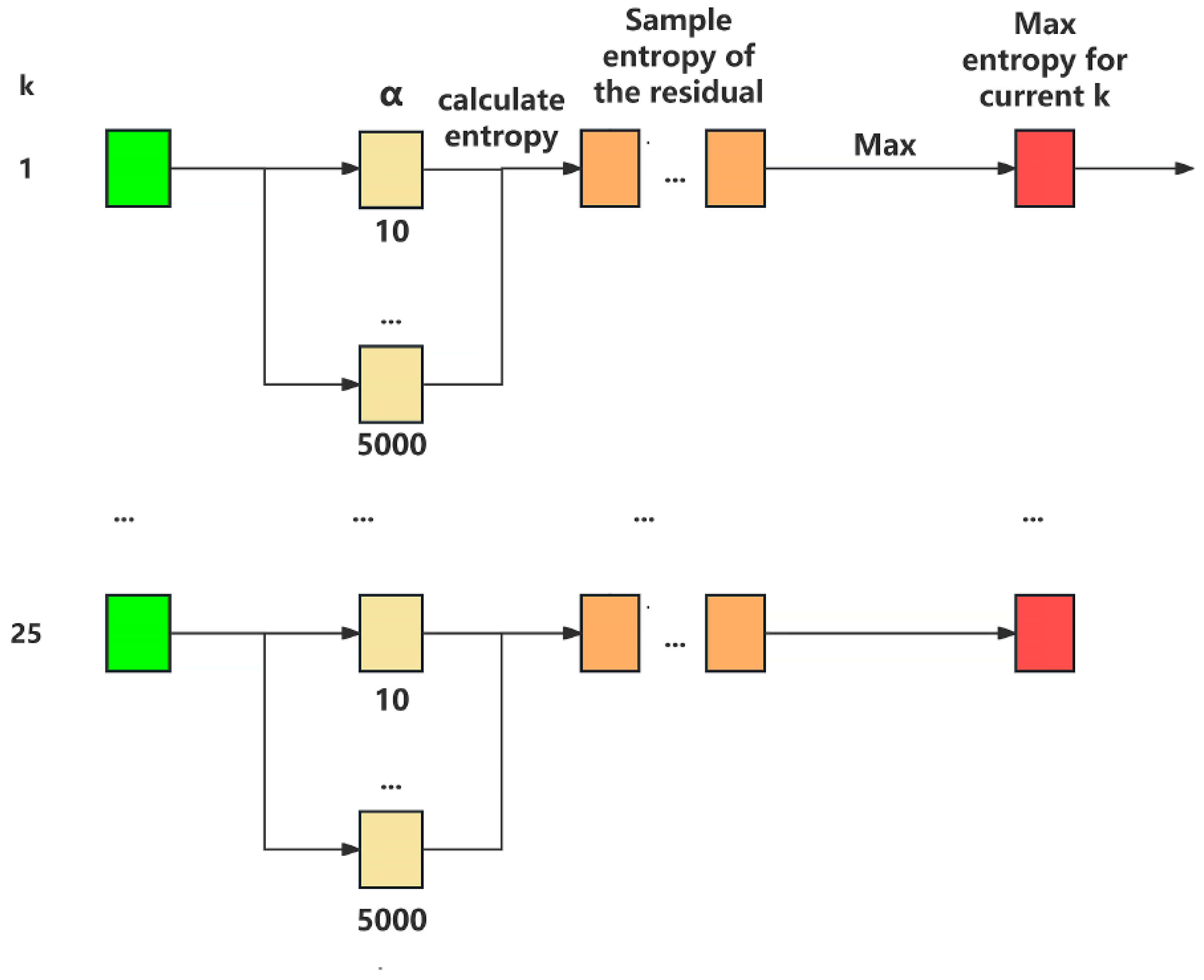
In order to calculate the sample entropy, a specific range was defined for both the decomposition level and the penalty factor with an enumeration of intervals. Considering the significant time cost associated with this process, we set the range of the penalty factor to (10, 5000) with an interval of 20, and the decomposition level was set to (1, 25) with an interval of 1. For each parameter combination defined by the decomposition levels and penalty factor, denoted as [k, α ], we obtain IMFs through the MVMD process. Subsequently, based on Equation (8), we aggregate the acquired IMFs and compute their difference from the original signal to derive the residual term. We then calculate the sample entropy of this residual term. Figure 1 illustrates the iterative process, where the yellow boxes represent a series of sample entropies calculated for an individual k value with multiple α values, and the red box indicates the maximum sample entropy for the current k value.

2.3. Combination of MVMD and TFT

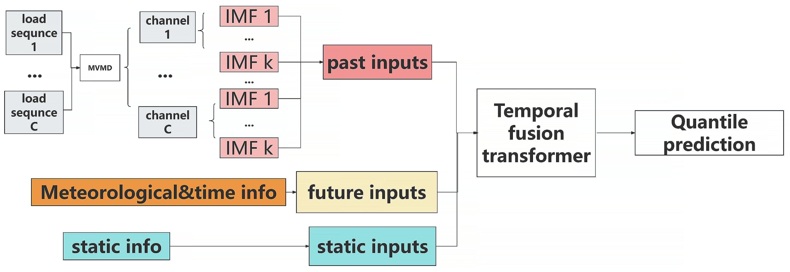
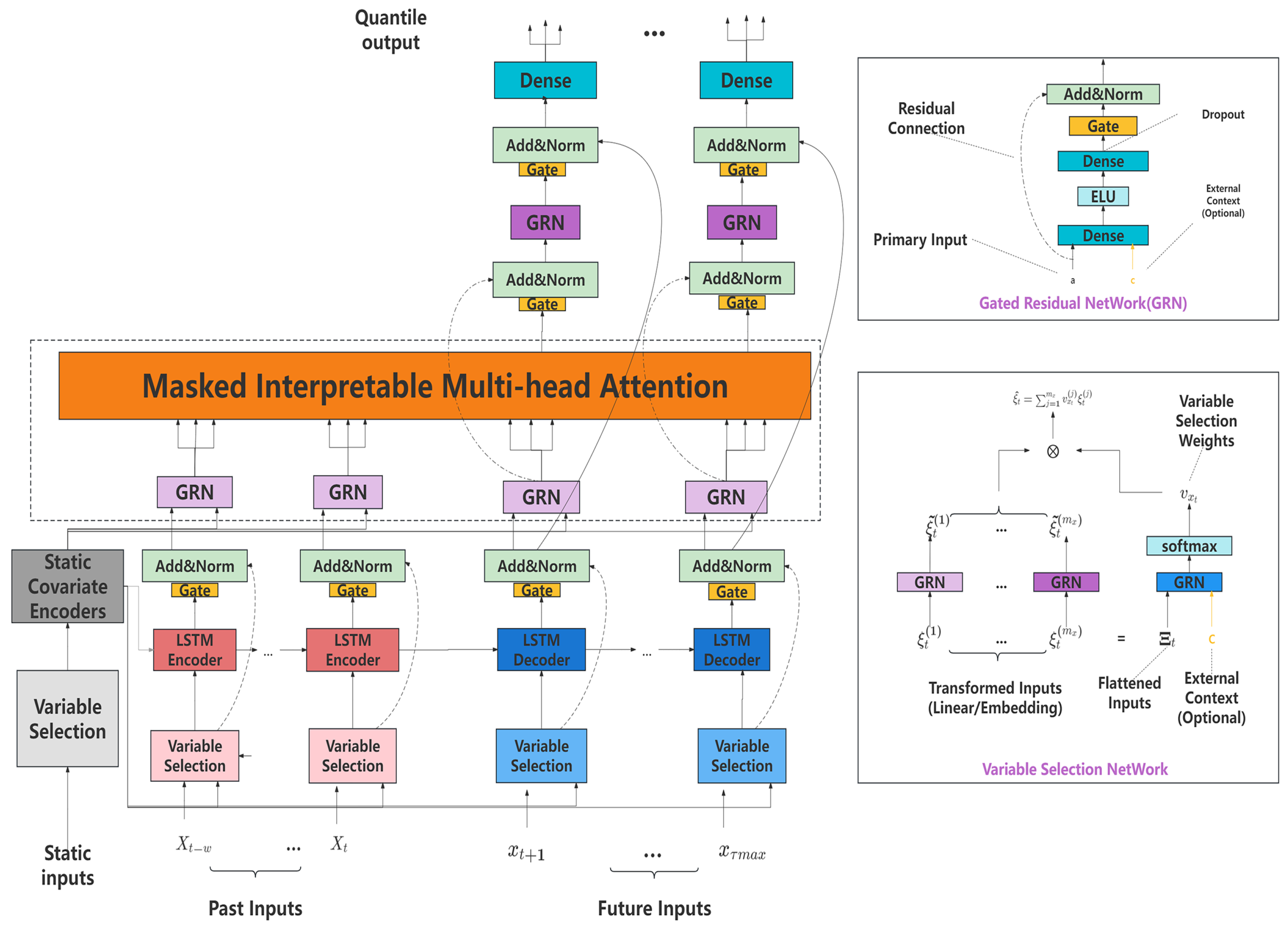
The TFT partitions the inputs into three distinct parts: the past input, the future input, and the static input, as illustrated in Figure 2. The past input can be represented as X ( t ) = [ X t w , X t ] , where the size of the look-back window is denoted by w. The future input, denoted as x ( t ) = [ x t + 1 , x t + τ ] , serves as a prior variable that resides within the same temporal range as the predicted target. Here, τ represents the forecast step, indicating the number of time units into the future that we aim to predict. The static input comprises variables that are independent of time.
The principle of the TFT is mainly composed of the following components:
(1)
Gated residual network: The GRN is designed to control the flexibility of nonlinear mapping in the model.
(2)
Variable selection network: The VSN is designed to provide instance-wise variable selection. It can learn the most salient input variable, which contributes to the prediction problem. It provides access to static information that enhances the weight-generation process.
(3)
Attention mechanism: The TFT applies an average attention mechanism that prevents the model from attending to different input features at different times and facilitates the evaluation of the importance of instance-wise attention weights.
(4)
Quantile loss: The TFT provides a distribution of possible future outcomes along with point estimates through quantile output, and it is trained using quantile loss. In our research, the quantile is set to {0.1, 0.5, 0.9}.
In order to enhance the ability of the TFT to simultaneously learn patterns from multiple load series, we introduced a novel approach by substituting the load series in past inputs with the results obtained from MVMD.
Figure 3 illustrates the integration of MVMD with the TFT. Consider a scenario with C load series and s exogenous variables, each having a length of L. The decomposition level of MVMD is set to k. After decomposition on the load series, a three-order matrix of dimensions [C, k, L] is obtained. In order to incorporate the past known input using LSTM, the decomposition matrix is reshaped into [ C × L , k]. By incorporating the exogenous variables, the final input matrix size becomes [ C × L , k + s ].

2.4. The Process of Optimizing MVMD-TFT Using WOA

The whale optimization algorithm (WOA) [26] is a nature-inspired optimization algorithm that mimics the foraging behavior of whales to solve complex optimization problems. The WOA introduces two strategies for position updates, which are intended to occur with equal probability. It ensures the exploration and exploitation of the search space.
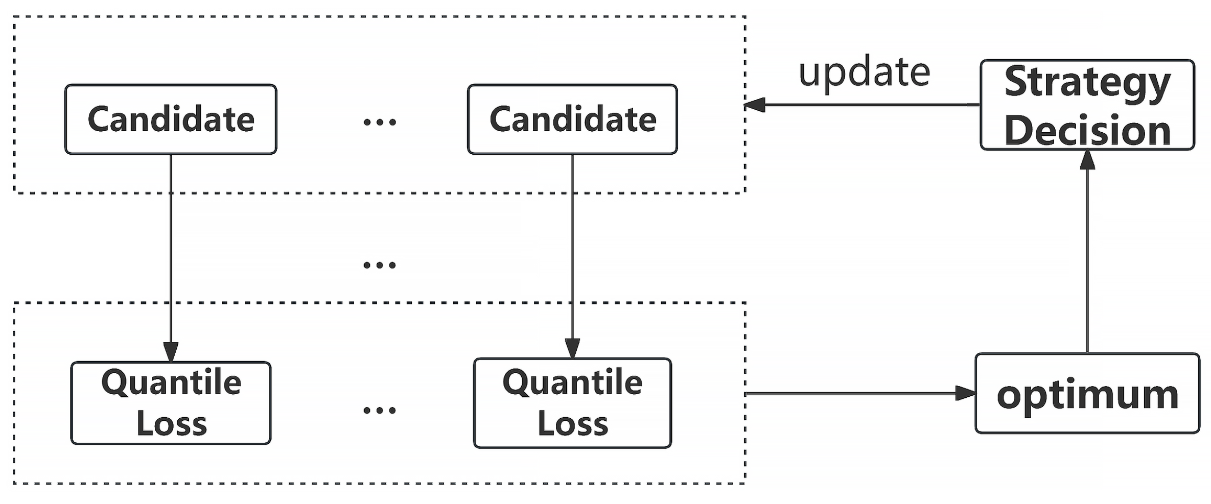
Strategy 1: Encircling prey. Suboptimal candidates update their positions based on a pair of cross-correlation vectors. The mathematical expression describing this update process is outlined in Equations (7) and (8):
X ( n + 1 ) = X * ( n ) A · D
X ( n + 1 ) = X r a n d ( n ) A · D
where n represents the current iterations, X represents the position of suboptimal candidates, and X * denotes the position of the current optimal candidate. Vector A , D denotes the coefficient vectors. The algorithm incorporates a random foraging strategy, which is related to the norm of A . If | A | > 1 , the position of the current optimal candidate is replaced with a randomly generated vector, and the remaining candidates are updated using Equation (8), with X r a n d denoting a randomly generated vector. Otherwise, Equation (7) is employed for updating.
Strategy 2: Bubble-net attacking method:
X ( n + 1 ) = | X * ( n ) X ( n ) | · e β l · cos ( 2 π l ) + X * ( n ) .
The suboptimal candidates update their position by calculating the distance between themselves and the optimal candidate. The mathematical expression is presented in Equation (9), where l represents a random number between [−1, 1] and β denotes a constant related to helicity.
Figure 4 depicts the process of optimizing MVMD-TFT hyperparameters with the WOA over one iteration. Initially, we establish the population size and boundary conditions, from which we derive the initial values of solution candidates. Subsequently, we feed the hyperparameter sets represented by each candidate into the TFT model for training, thereby acquiring the quantile loss specific to each individual. Based on the results of quantile loss, we determine the current optimal individual and randomly select the strategy to update the candidates.

3. Results and Discussion

3.1. Experimental Setup

The environment used in this experiment is TensorFlow 2.5, Python 3.8, and a single RTX2080Ti. We implemented the Python version of MVMD by referring to vmdPy and MVMD source code.

3.2. Data Preprocessing

The datasets utilized in this study were obtained from BCHydro [27], encompassing the hourly electricity consumption of 28 residential customers. The consumption data span 3 years. The meteorological data from neighboring weather stations was also incorporated. The temporal boundaries for energy consumption data vary among the 28 buildings in the original dataset, making it impractical to use the entire dataset for training purposes. In order to ensure the selection of appropriate buildings and time frames from the original dataset, we applied the following criteria:
(1)
In order to minimize the missing values within the selected time range, we have stipulated that the proportion of missing values for all variables employed in model training within the specified time range be less than 0.5%. Variables exceeding this missing value threshold were excluded from consideration. In order to facilitate a comparison between LSTM and CNN-LSTM, we opted for two non-overlapping time ranges. One time range spans approximately 3 months (1 November 2017 to 29 January 2018) (Case A), similar to [7], while the second time range encompasses roughly 16 months (26 June 2016 to 30 October 2017) (Case B).
(2)
The meteorological data for the selected buildings all originate from the same weather station. Additionally, each building is accompanied by its corresponding descriptive information. Buildings that have incomplete descriptions are excluded from the analysis. Following the aforementioned criteria, Case A comprises 14 buildings, while Case B includes 10 buildings.
For cases A and B, we applied a consistent data processing methodology, which can be summarized as follows. For Case A, we first aggregated the data from different buildings. Next, we added the “building_id” feature to distinguish the load of different buildings. For the data from each building, we constructed training, validation, and test sets in an 8:1:1 ratio. Then, we performed MVMD decomposition on the load part of these three parts of the data separately. After that, we processed the training set of each building based on “building_id” using Equation (10) and obtained the corresponding maximum and minimum values. We then normalized the test set and validation set using the maximum and minimum values obtained from the training set.
Table 1 presents the variables that were selected as inputs for our model, taking into consideration the criteria based on the number of missing values.
M i n M a x S c a l e r ( x ) = x min ( x ) max ( x ) min ( x )

3.3. Entropy Computation Results of MVMD

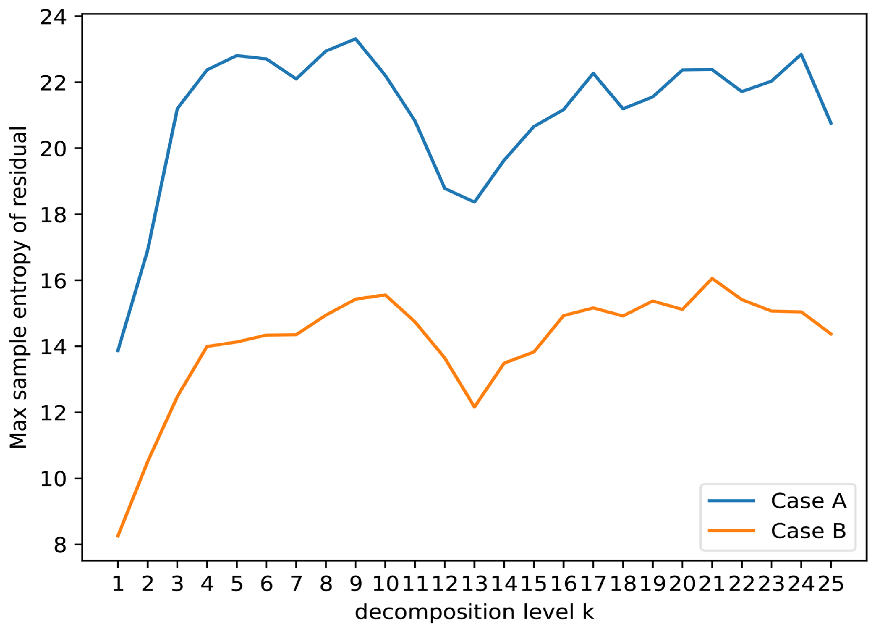
Figure 5 displays the results of residual sample entropy obtained by selecting the optimal penalty factor α for two training set cases (red boxes in Figure 1). We find that the residual sample entropy of Case B is lower than that of Case A, implying that the signal patterns in Case B are more intricate, resulting in lower residual complexity.
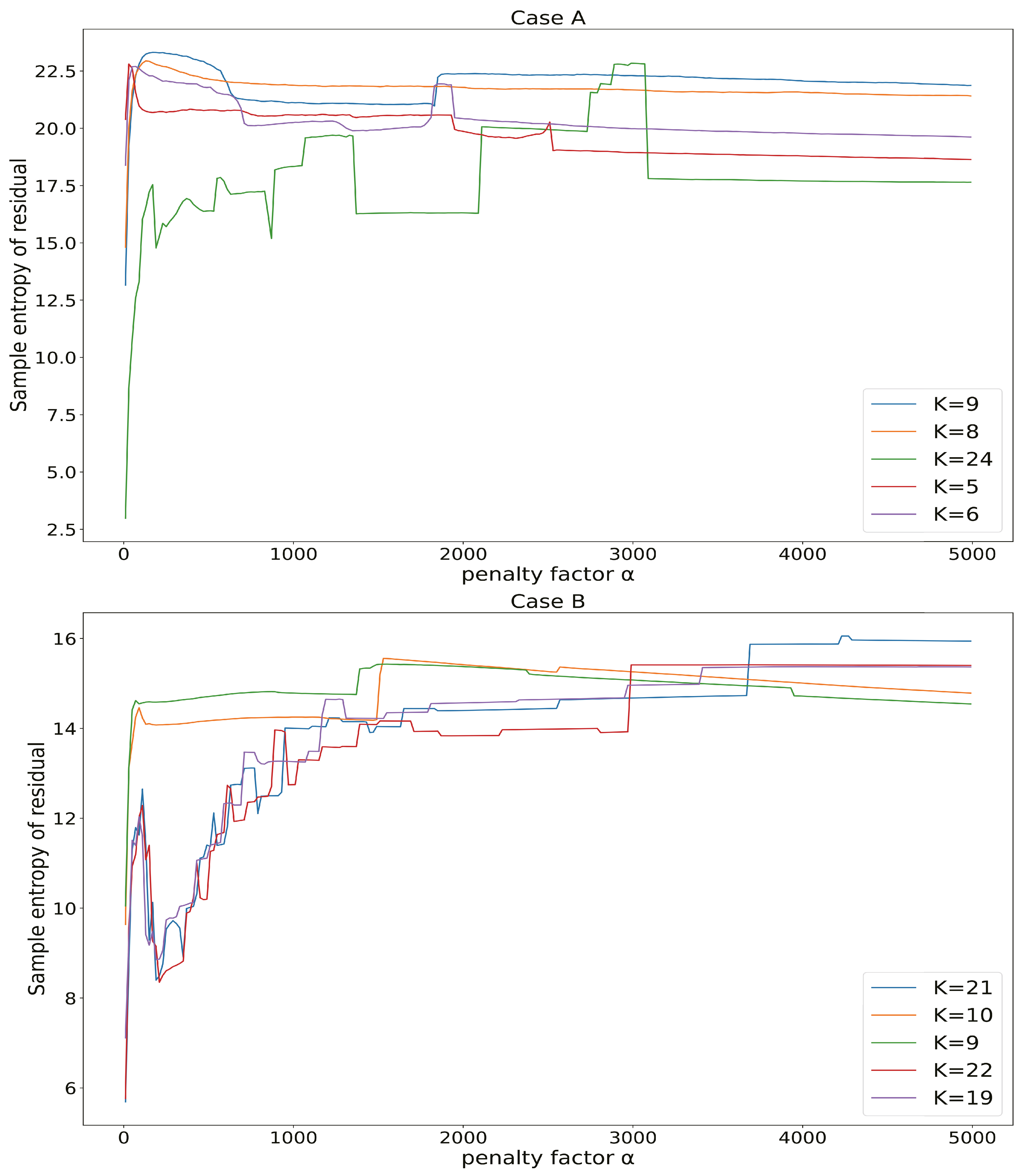
Figure 6 illustrates the impact of different penalty factors on residual sample entropy (yellow boxes in Figure 1) for the same decomposition level. We selected five decomposition levels for analysis based on their highest residual sample entropy. The introduction of the penalty factor leads to complexity in the pattern of residual sample entropy. Specifically, we observe pronounced fluctuations in residual sample entropy for higher decomposition levels under varying penalty factors, for instance, in Case A, when the decomposition level was set to 24, and in Case B, when the decomposition level was set to 21, 22, and 19. These fluctuations gradually diminish as the penalty factor increases, eventually reaching a relatively stable state. Based on these findings, for Case A, the decomposition level was set to 9, with a corresponding penalty factor of 170. For Case B, the decomposition level was set to 21, with a corresponding penalty factor of 4230. The initial center frequency of MVMD is initialized using a uniform distribution, and the tolerance level is set to 1 × 10⁻⁶.
For the test set and validation set, we similarly obtained their optimal penalty factors based on Figure 1 while maintaining the same number of decomposition levels as the training set. The penalty factors for the validation set and test set in Case A were set as 1230 and 1240, respectively. For Case B, the penalty factors for the validation set and test set were set as 3410 and 4030, respectively.

3.4. Optimization Results Using WOA

In order to enhance the performance of the MVMD-TFT model, we employed the WOA to optimize its hyperparameters. In this paper, we set the population size and number of iterations for the WOA to 10, taking into account the significant computational cost associated with the TFT training.
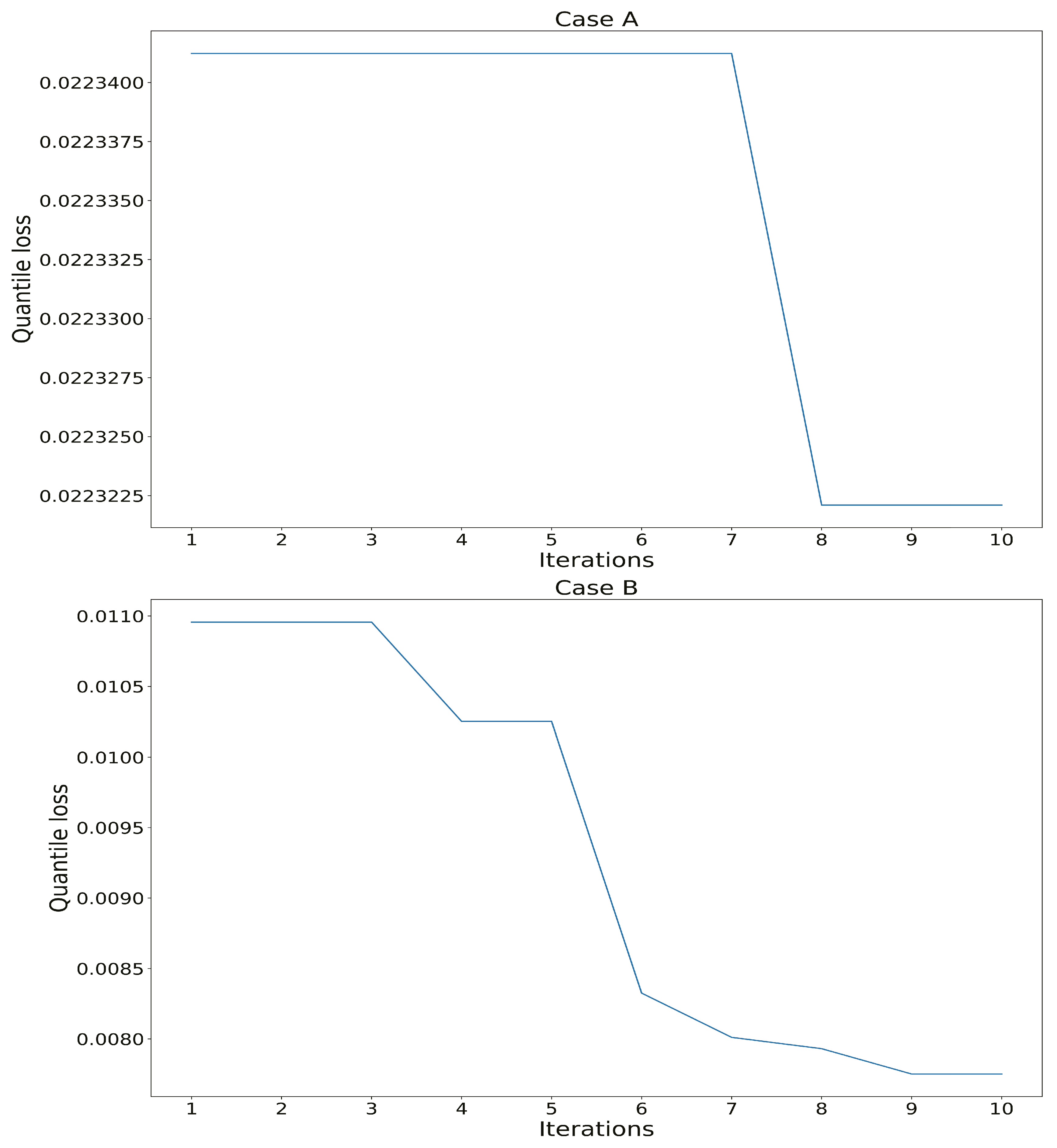
Figure 7 shows the optimal value obtained in each iteration from the WOA. In case A, during 10 iterations, the quantile loss was only optimized once, and the difference between the optimized loss and the previous loss was relatively small. In Case B, the quantile loss was optimized five times, with the resulting loss being lower than that of Case A. The hyperparameters of the optimized MVMD-TFT and corresponding search range are shown in Table 2.

3.5. Interpretability of MVMD-TFT

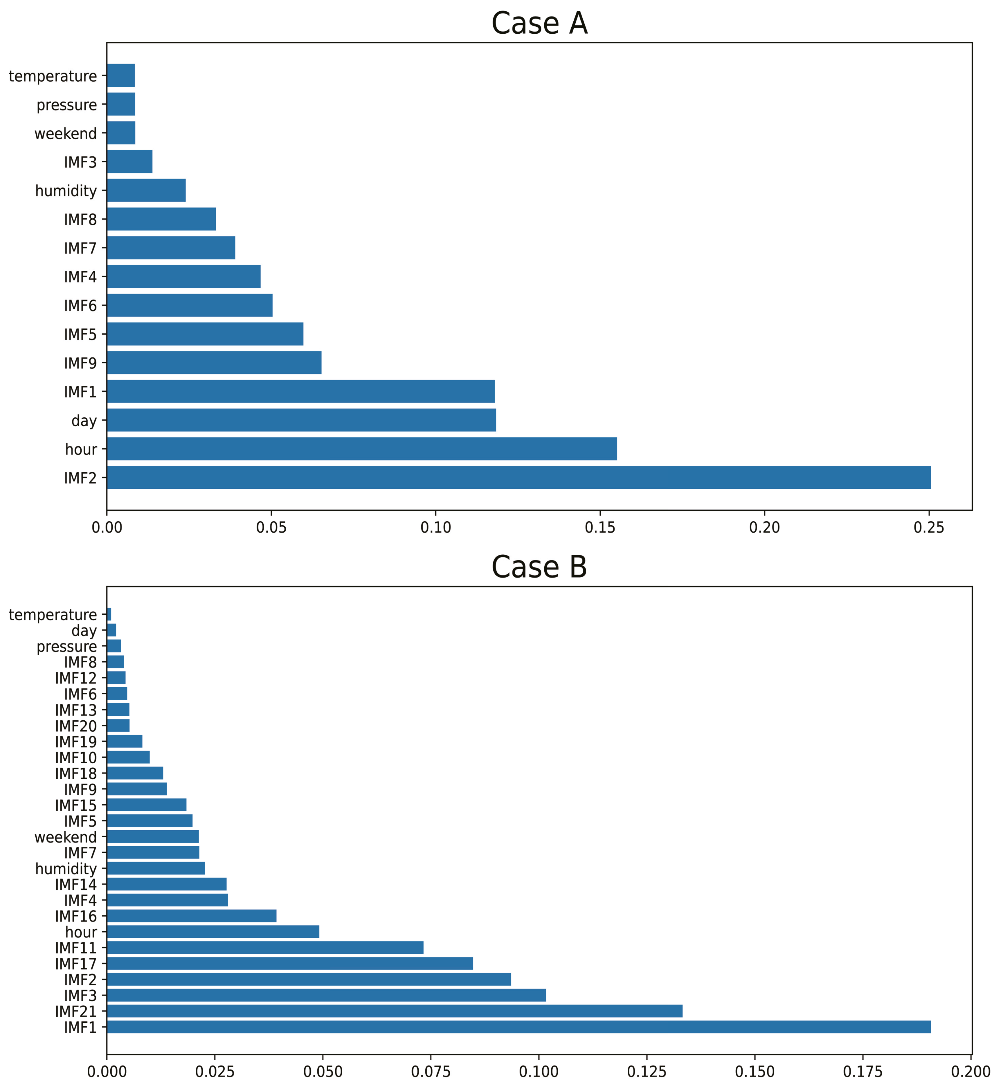
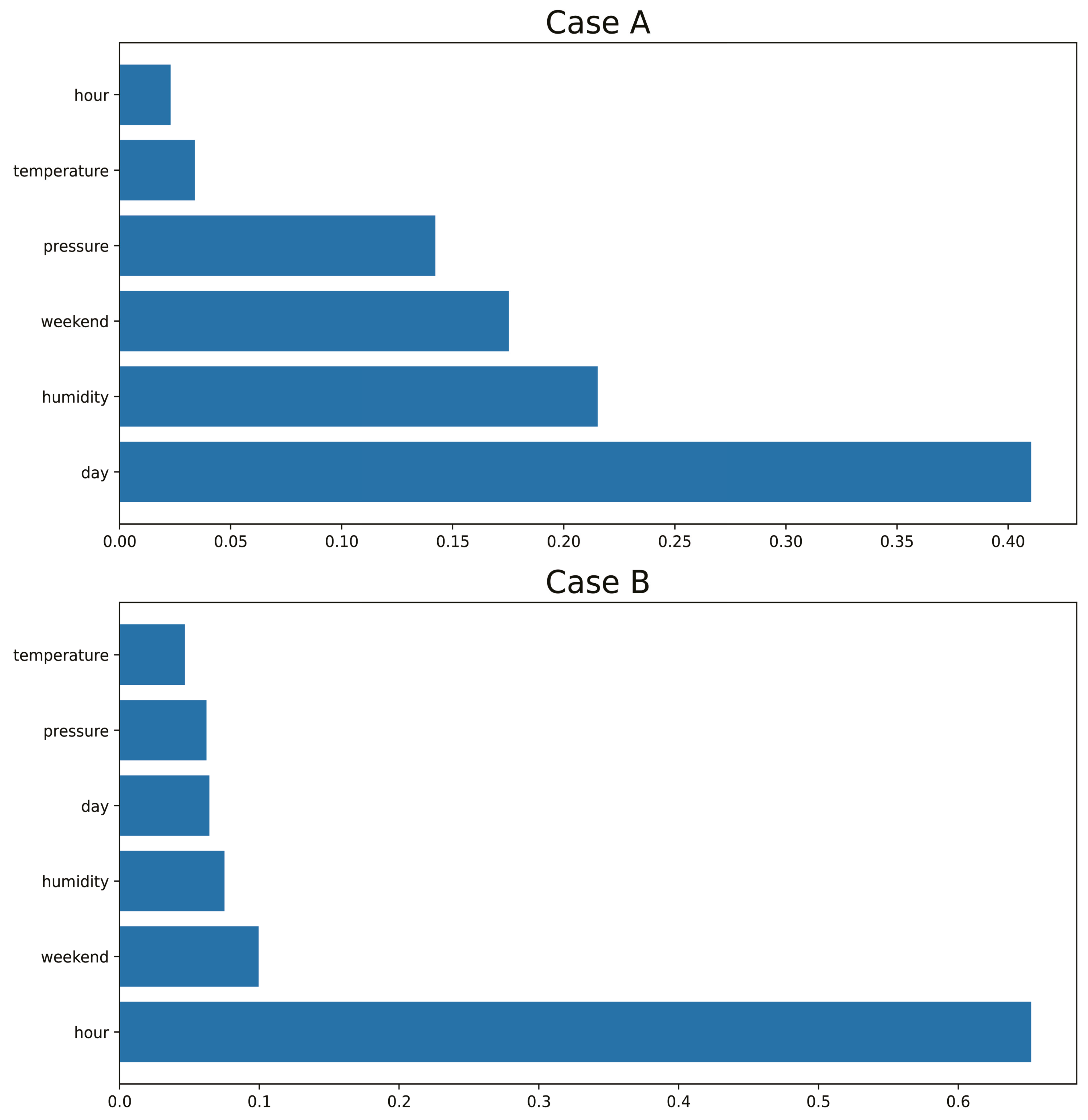
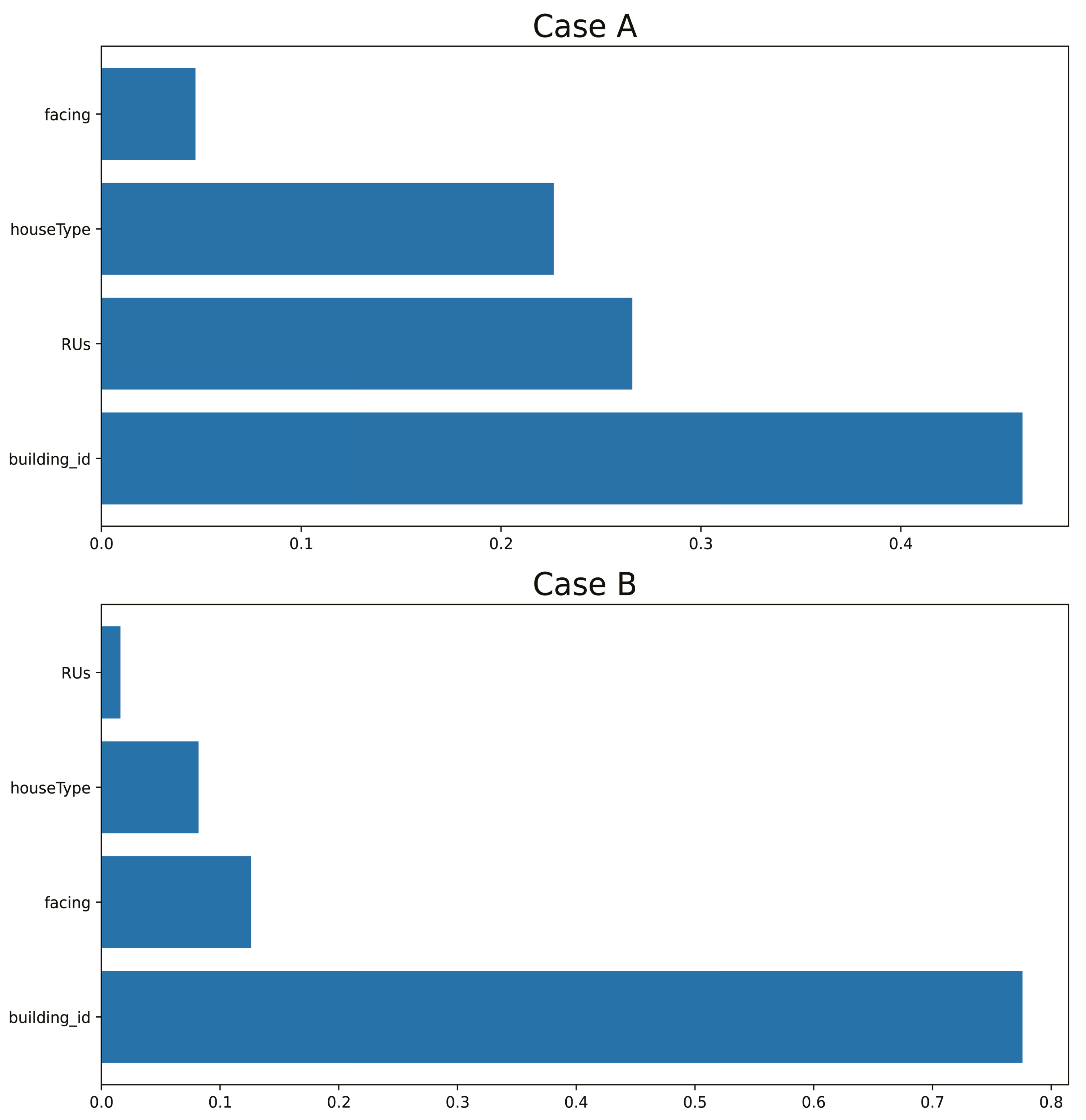
The TFT gives the interpretability between the input and output variables through the calculation in VSN. The results are presented in Figure 8, Figure 9 and Figure 10.
Figure 8 illustrates the weight distribution of VSN in past inputs, indicating that the IMFs obtained from MVMD emerge as a crucial factor, demonstrating a notable level of significance. Figure 9 illustrates the weight distribution of the VSN in future inputs, highlighting the significant roles played by the time indicators ‘day’ and ‘hour’. Figure 10 presents the weight distribution of the VSN in static inputs, emphasizing ‘building_id’ as the most prominent feature.

3.6. Model Evaluation

For performance comparisons, we employed LSTM [6], CNN-LSTM, [7] and BiGRU-CNN [28]. A distinct model was trained for each building using these methods. In order to ensure consistency with the reference, we adopted the original preprocessing method, which involved representing the time indicator using one-hot encoding. The input for these models consisted of both time indicators and load series, enabling a comprehensive analysis of their predictive capabilities. Additionally, we conducted a comparative analysis with separately trained MVMD-LSTM and MVMD-CNN-LSTM models to further substantiate the efficacy of our method. The implementation of these standalone models followed the methodology outlined in [29], employing LSTM and CNN-LSTM architectures for the prediction of the IMFs and the subsequent reconstruction of the predicted signals. Concerning the CNN-LSTM-based, LSTM-based, and BiGRU-CNN models, we incorporated one of the lag inputs specified in [7]. Specifically, we configured it to 12. As a preliminary trial for the TFT and MVMD-TFT models, we utilized 24 lag inputs. Table 3 displays other configurations of the models.
As our data contain both outliers and stable points, we utilized Equations (11)–(14) to evaluate the performance of the models, where y i represents the actual value, and y i ^ denotes the predicted value. MAE and MSE are the two most commonly used metrics in predictive problems, with MSE being more sensitive to outliers relative to MAE. MedAE serves as a robust measure of the variability of deviation of the observed values from the predict values. Additionally, we introduce WAPE to measure the percentage difference between actual and predicted values, as our data contain zeros, making this metric an alternative to MAPE. These four metrics provide different perspectives on the model’s performance. All methods exhibit a prediction horizon of 1, meaning that the predicted results correspond to the consumption data for the next hour. We made the original building name more concise by simplifying ‘Residential_’ to ‘R’.
M A E = 1 N Σ i = 1 N | y i y i ^ |
M S E = 1 N Σ i = 1 N ( y i y i ^ ) 2
W A P E = Σ i = 1 N | y i y i ^ | Σ i = 1 N | y i |
M e d A E = m e d i a n ( | y 1 y 1 ^ | , , | y i y i ^ | )
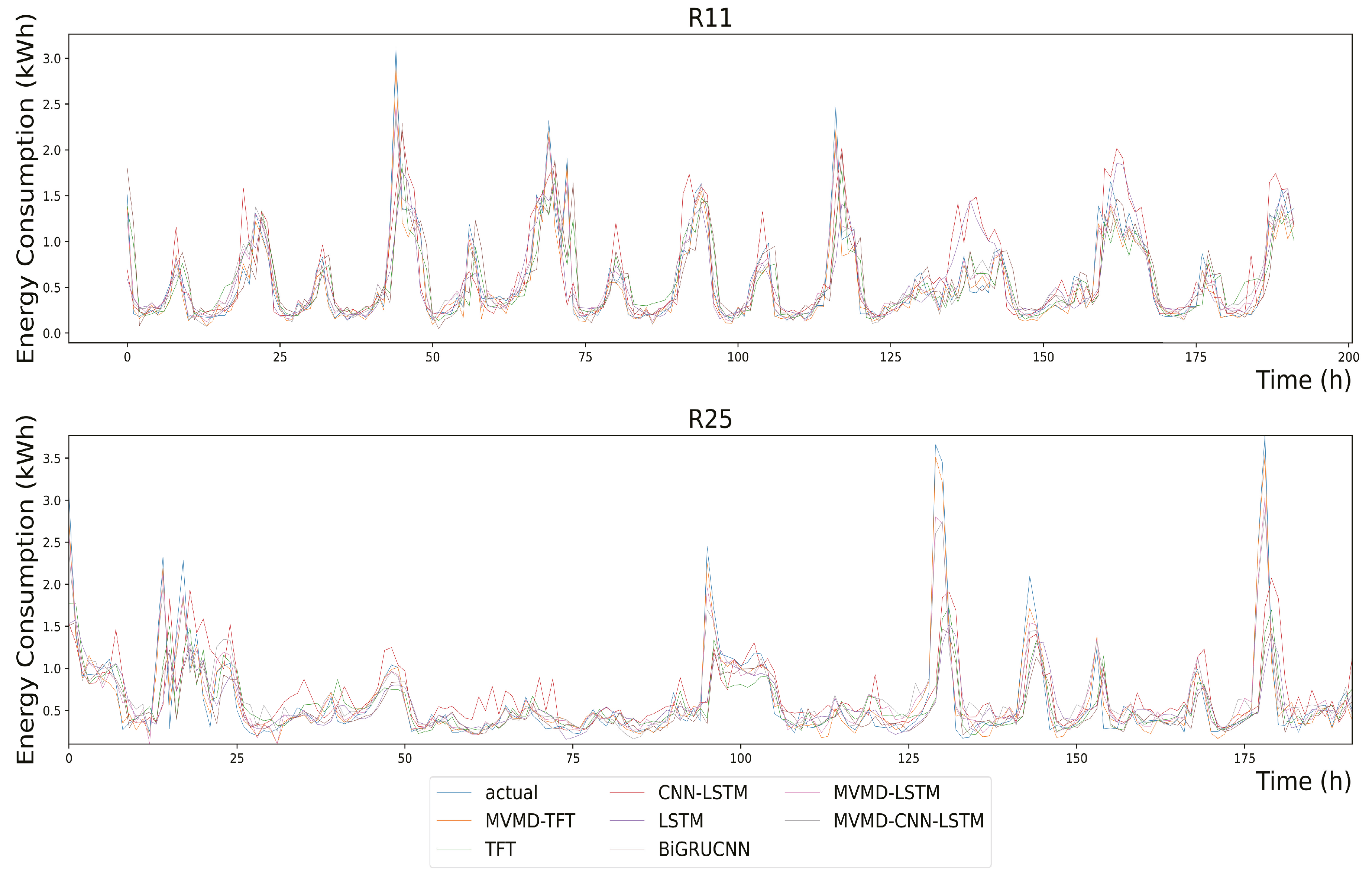
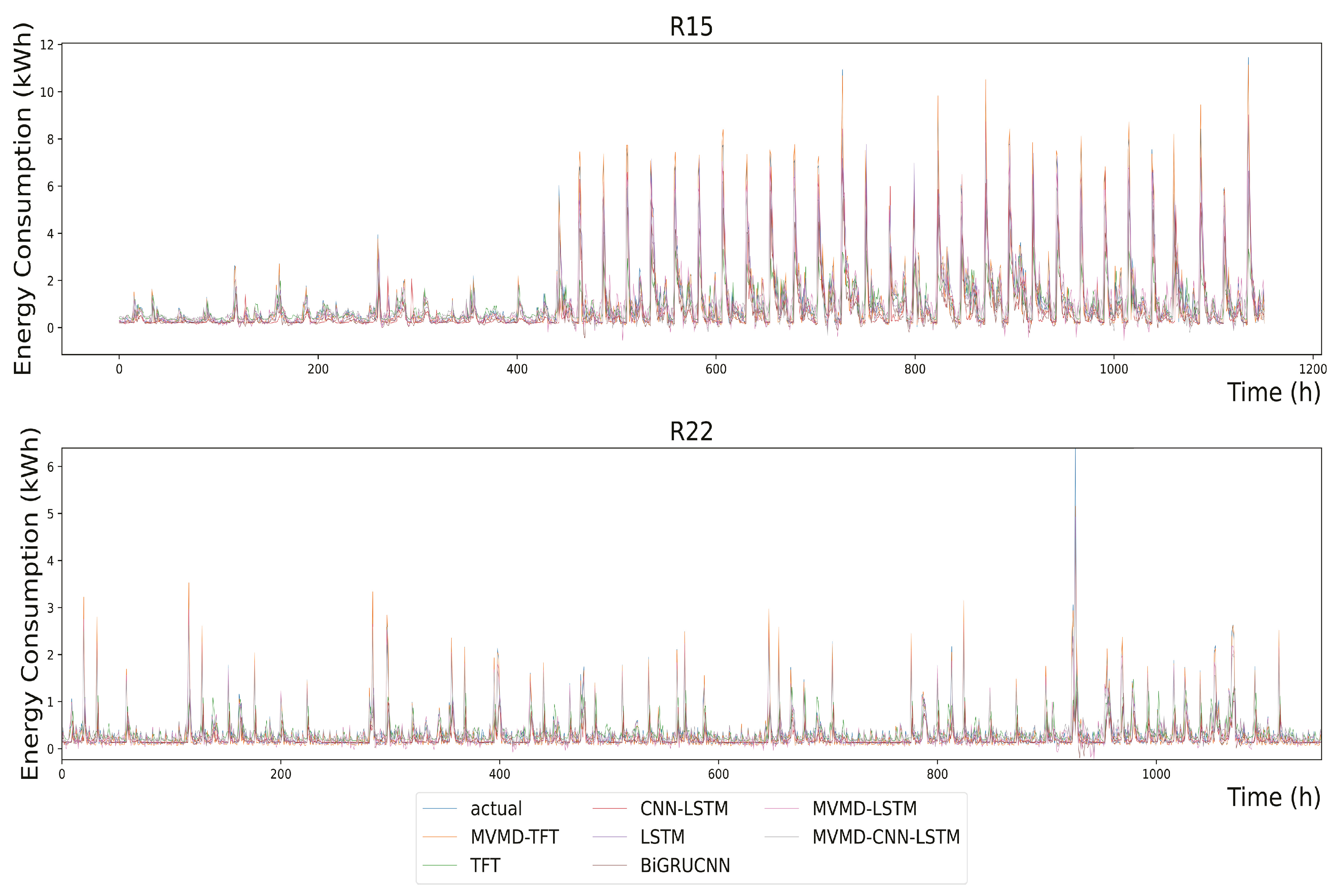
Table 4 illustrates the prediction errors associated with Case A on the test set. The results show that the introduction of MVMD yielded substantial improvements in the performance of the CNN-LSTM, LSTM, and TFT models. A consistent decrease in all metrics shows this enhancement. Figure 11 depicts the corresponding prediction outcomes of ‘R11’ and ‘R24’ in Table 4, where the TFT and MVMD-TFT employ median forecasting. Table 5 illustrates the four loss function outcomes for Case B on the test set. We can derive similar conclusions to those of Case A when the dataset expands. It is worth noting that certain buildings, such as R13 and R5, demonstrate elevated MSE values that surpass the corresponding MAE values. After undergoing MVMD and subsequent prediction, it is observed that the MSE decreases to a level smaller than that of the MAE. This reveals that the implementation of MVMD preprocessing effectively attenuates the deleterious impact of outliers on predictive outcomes. Figure 12 aligns with the predictions of ‘R15’ and ‘R22’ outlined in Table 4.
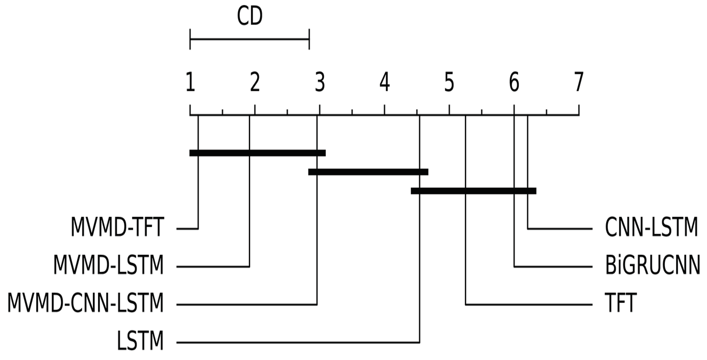
The results in Table 4 and Table 5 reveal a similarity in the experimental outcomes between the MVMD-based models. In order to establish the statistical significance of the results displayed in Table 4 and Table 5, we introduce the Friedman and post-hoc Nemenyi tests [30] to assess the differences among various models for evaluation. The null hypothesis of the Friedman test is that there is no difference among all comparison methods in the 24 datasets of Case A and Case B. We set the p-value to be 0.05. If the calculation result of the Friedman test is less than 0.05, the null hypothesis is rejected; otherwise, it indicates a difference between the methods. Furthermore, to assess the performance between pairwise models, we introduced the Nemenyi post-hoc test. This test launches a comparison between a threshold (critical difference) and the difference in average rankings of the performance. If the ranking difference is lower than the threshold, it is considered that there is no significant difference in performance between the pairwise models. On the contrary, there is a significant performance difference between them. The evaluation metric of the Nemenyi test is MAE.
After performing the calculations on 24 datasets, we obtained a p-value of 5.3 × 10⁻¹⁹ for the Friedman test. This is significantly lower than the preset threshold of 0.05, indicating a significant difference in performance among the seven methods.
Figure 13 displays the results of the Nemenyi post-hoc tests, with a calculated CD value of 1.84. The results of the Nemenyi tests indicate that there are no significant differences in the performances of the CNN-LSTM, TFT, LSTM, and BiGRU-CNN. In the case of the MVMD-TFT, it shows differences with all non-MVMD-based methods. Based on the results from Table 4 and Table 5, our method achieved an average reduction of 69.9% in MAE for an individually trained CNN-LSTM and BiGRU-CNN, as well as a 67.7% reduction in MAE for an individually trained LSTM. Although no significant performance differences were detected for the MVMD-based methods, the proposed method demonstrated the best performance in the current experiment.
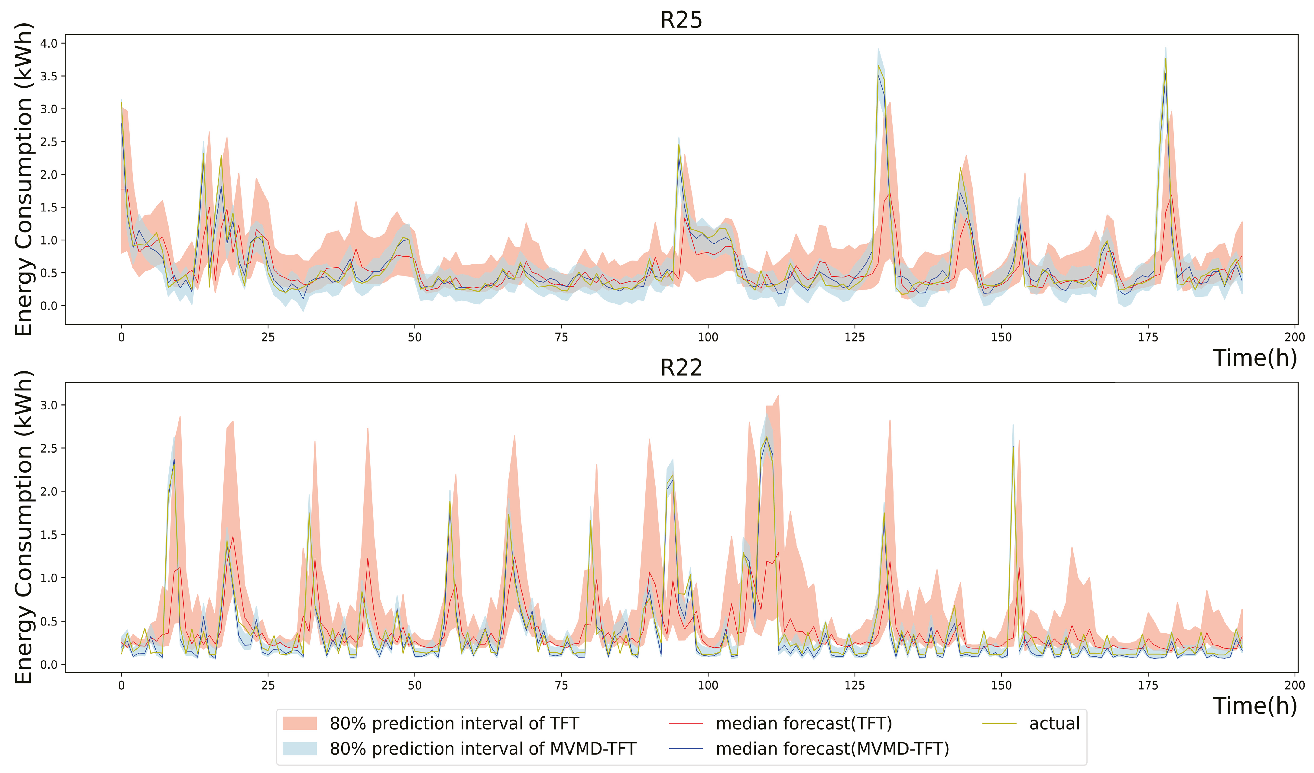
One of the important features of the TFT is that it provides a distribution of possible future outcomes along with point estimates, which is valuable for understanding the uncertainty associated with each prediction. Given that our model utilizes a quantile set of (0.1, 0.5, 0.9), the TFT produces a prediction interval of 80%. Figure 14 presents both the median prediction results and their associated 80% prediction interval in two chosen buildings where peak values are observed. The results reflect the last 8 days from the entire test set. The proposed model attains a narrower prediction interval than the original method and is more likely to encompass peak values.
q -Risk = 2 Σ i , t Q L ( y i , y i ^ , q ) Σ i , t | y i |
In order to perform a thorough assessment of the quantile forecast, we utilized the P50 loss and P90 loss, as specified in [31] and described in Equation (15). In the context of the 8-day evaluation, the test set comprises a total of 192 data points. Equation (15) is applied to compute the q-Risk value for each data point in the 1-hour-ahead forecast. Consequently, the average quantile loss for the 192 points was derived.
Table 6 showcases the average q-Risk value for the forecast of the MVMD-TFT and TFT across all points in both cases. The results show that our method yields 75.9% lower P90 loss and 65.8% lower P50 loss on average, providing additional evidence for the effectiveness of our method.
Although our method has successfully produced accurate predictions in two instances, it is burdened by substantial time-related limitations that cannot be ignored. This deficiency is particularly evident in the WOA, where the computational demands of the TFT impose limitations on the selection of optimal initial parameters for the WOA. Consequently, the convergence of the WOA is insufficient, with the magnitude of this flaw becoming increasingly apparent as the dataset size and model complexity grow. Moreover, our method incorporates MVMD, which requires substantial time in data preprocessing to ascertain the most appropriate parameters. The determination of the parameters of the two cases together is approximately seven days. These limitations underscore the need for further improvements in our approach to address the substantial time constraints associated with the optimization process for the TFT and MVMD.
4. Conclusions

In this paper, we propose a novel MVMD-WOA-TFT hybrid model for accurate hourly load consumption forecasting across multiple houses. MVMD is leveraged to decompose the original load series into multiple IMFs. This enables the extraction of shared characteristics from various load series, thereby assisting the TFT in comprehending the underlying patterns and relationships among different load sequences. In order to select a suitable decomposition level and penalty factors for MVMD, we employed a method that maximizes the sum of the residual sample entropy, as a higher entropy signifies a better decomposition by capturing more noise in the residual. Subsequently, we partitioned the dataset into training, validation, and test sets and performed separate decompositions on each. The WOA was employed to determine the hyperparameters of the MVMD-TFT model, improving its overall performance. We used separately trained LSTM, CNN-LSTM, BiGRU-CNN, MVMD-LSTM, and MVMD-CNN-LSTM models for performance comparisons. Our approach exhibits competitive performance compared to MVMD-LSTM and MVMD-CNN-LSTM for the 24 datasets, but it achieved excellent performance with the non-MVMD method. Our method achieved an average reduction of 69.9% for CNN-LSTM and BiGRU-CNN, as well as a 67.7% reduction for LSTM in MAE. We conducted additional evaluations on quantile predictions for the TFT, achieving an average improvement of 65.8% at 0.5 risk and 75.9% at 0.9 risk. However, it is worth noting that the three processes (MVMD, WOA, and TFT) involved in our methodology entail a high computational cost. Additionally, our study only focused on 1-hour-ahead prediction and utilized fixed lag inputs to examine the prediction accuracy. Research is warranted to examine the influence of lag inputs and variations in the prediction range on the performance of the model.

Author Contributions

Conceptualization, Q.Z. and X.Z.; methodology, H.Y. and Q.Z.; software, H.Y.; validation, H.Y. and Q.Z.; formal analysis, H.Y.; resources, X.Z.; writing—original draft preparation, H.Y.; writing—review and editing, Q.Z. and X.Z.; supervision, X.Z. All authors have read and agreed to the published version of the manuscript.

Funding

This research received no external funding.

Institutional Review Board Statement

Not applicable.

Informed Consent Statement

Not applicable.

Data Availability Statement

Data are contained within the article.

Conflicts of Interest

The authors declare no conflicts of interest.

Abbreviations

The following abbreviations are used in this manuscript:
AdaBoostAdaptive boosting
ADMMAlternating direction method of multipliers
ARIMAAutoregressive integrated moving average
BiGRUBidirectional Gated recurrent unit network
BiLSTMBidirectional long short-term memory network
CDCritical Difference
CNNConvolutional neural network
DBSCANDensity-based spatial clustering of applications with noise
EEMDEnsemble empirical mode decomposition
ELMExtreme learning machine
EMDEmpirical mode decomposition
EWTEmpirical wavelet transform
GRUGated recurrent unit network
IMFIntrinsic mode function
LSSVMLeast squared support vector machine
LSTMLong short-term memory network
MAEMean absolute error
MAPEMean absolute percentage error
MedAEMedian absolute error
MLRMultiple linear regression
MSEMean squared error
MVMDMultivariate variational mode decomposition
RNNRecurrent neural network
SVRSupport vector regression
TFTTemporal fusion transformer
VMDVariational mode decomposition
VSNVariable selection network
WAPEWeighted average percentage error
XGBoostExtreme gradient boosting

References

  1. González-Torres, M.; Pérez-Lombard, L.; Coronel, J.F.; Maestre, I.R.; Yan, D. A review on buildings energy information: Trends, end-uses, fuels and drivers. Energy Rep. 2022, 8, 626–637. [Google Scholar] [CrossRef]
  2. Guo, X.; Gao, Y.; Li, Y.; Zheng, D.; Shan, D. Short-term household load forecasting based on Long- and Short-term Time-series network. Energy Rep. 2021, 7, 58–64. [Google Scholar] [CrossRef]
  3. Al-Rakhami, M.; Gumaei, A.; Alsanad, A.; Alamri, A.; Hassan, M.M. An Ensemble Learning Approach for Accurate Energy Load Prediction in Residential Buildings. IEEE Access 2019, 7, 48328–48338. [Google Scholar] [CrossRef]
  4. Chen, S.; Zhou, X.; Zhou, G.; Fan, C.; Ding, P.; Chen, Q. An online physical-based multiple linear regression model for building’s hourly cooling load prediction. Energy Build. 2022, 254, 111574. [Google Scholar] [CrossRef]
  5. Chen, Y.; Xu, P.; Chu, Y.; Li, W.; Wu, Y.; Ni, L.; Bao, Y.; Wang, K. Short-term electrical load forecasting using the Support Vector Regression (SVR) model to calculate the demand response baseline for office buildings. Appl. Energy 2017, 195, 659–670. [Google Scholar] [CrossRef]
  6. Kong, W.; Dong, Z.Y.; Jia, Y.; Hill, D.J.; Xu, Y.; Zhang, Y. Short-Term Residential Load Forecasting Based on LSTM Recurrent Neural Network. IEEE Trans. Smart Grid 2019, 10, 841–851. [Google Scholar] [CrossRef]
  7. Alhussein, M.; Aurangzeb, K.; Haider, S.I. Hybrid CNN-LSTM Model for Short-Term Individual Household Load Forecasting. IEEE Access 2020, 8, 180544–180557. [Google Scholar] [CrossRef]
  8. Peng, C.; Tao, Y.; Chen, Z.; Zhang, Y.; Sun, X. Multi-source transfer learning guided ensemble LSTM for building multi-load forecasting. Expert Syst. Appl. 2022, 202, 117194. [Google Scholar] [CrossRef]
  9. Zhu, N.; Wang, Y.; Yuan, K.; Yan, J.; Li, Y.; Zhang, K. GGNet: A novel graph structure for power forecasting in renewable power plants considering temporal lead-lag correlations. Appl. Energy 2024, 364, 123194. [Google Scholar] [CrossRef]
  10. Rumbe, G.; Hamasha, M.; Mashaqbeh, S.A. A comparison of Holts-Winter and Artificial Neural Network approach in forecasting: A case study for tent manufacturing industry. Results Eng. 2024, 21, 101899. [Google Scholar] [CrossRef]
  11. Tarmanini, C.; Sarma, N.; Gezegin, C.; Ozgonenel, O. Short term load forecasting based on ARIMA and ANN approaches. Energy Rep. 2023, 9, 550–557. [Google Scholar] [CrossRef]
  12. Mounir, N.; Ouadi, H.; Jrhilifa, I. Short-term electric load forecasting using an EMD-BI-LSTM approach for smart grid energy management system. Energy Build. 2023, 288, 113022. [Google Scholar] [CrossRef]
  13. Yuan, J.; Wang, L.; Qiu, Y.; Wang, J.; Zhang, H.; Liao, Y. Short-term electric load forecasting based on improved Extreme Learning Machine Mode. Energy Rep. 2021, 7, 1563–1573. [Google Scholar] [CrossRef]
  14. Short-Term Load Forecasting Method Based on EWT and IDBSCAN. J. Electr. Eng. Technol. 2020, 15, 58–64.
  15. Lv, L.; Wu, Z.; Zhang, J.; Zhang, L.; Tan, Z.; Tian, Z. A VMD and LSTM Based Hybrid Model of Load Forecasting for Power Grid Security. IEEE Trans. Ind. Inform. 2022, 18, 6474–6482. [Google Scholar] [CrossRef]
  16. Lusis, P.; Khalilpour, K.R.; Andrew, L.; Liebman, A. Short-term residential load forecasting: Impact of calendar effects and forecast granularity. Appl. Energy 2017, 205, 654–669. [Google Scholar] [CrossRef]
  17. Kong, W.; Dong, Z.Y.; Hill, D.J.; Luo, F.; Xu, Y. Short-Term Residential Load Forecasting Based on Resident Behaviour Learning. IEEE Trans. Power Syst. 2018, 33, 1087–1088. [Google Scholar] [CrossRef]
  18. Huy, P.C.; Minh, N.Q.; Tien, N.D.; Anh, T.T.Q. Short-Term Electricity Load Forecasting Based on Temporal Fusion Transformer Model. IEEE Access 2022, 10, 106296–106304. [Google Scholar] [CrossRef]
  19. López Santos, M.; García-Santiago, X.; Echevarría Camarero, F.; Blázquez Gil, G.; Carrasco Ortega, P. Application of Temporal Fusion Transformer for Day-Ahead PV Power Forecasting. Energies 2022, 15, 5232. [Google Scholar] [CrossRef]
  20. Wu, B.; Wang, L.; Zeng, Y. Interpretable wind speed prediction with multivariate time series and temporal fusion transformers. Energy 2022, 252, 123990. [Google Scholar] [CrossRef]
  21. Feng, G.; Zhang, L.; Ai, F.; Zhang, Y.; Hou, Y. An Improved Temporal Fusion Transformers Model for Predicting Supply Air Temperature in High-Speed Railway Carriages. Entropy 2022, 24, 1111. [Google Scholar] [CrossRef] [PubMed]
  22. Wu, B.; Wang, L.; Zeng, Y.R. Interpretable tourism demand forecasting with temporal fusion transformers amid COVID-19. Appl. Intell. 2023, 53, 14493–14514. [Google Scholar] [CrossRef] [PubMed]
  23. Wu, B.; Wang, L.; Tao, R.; Zeng, Y.R. Interpretable tourism volume forecasting with multivariate time series under the impact of COVID-19. Neural Comput. Appl. 2023, 35, 5437–5463. [Google Scholar] [CrossRef]
  24. Rehman, N.U.; Aftab, H. Multivariate Variational Mode Decomposition. IEEE Trans. Signal Process. 2019, 67, 6039–6052. [Google Scholar] [CrossRef]
  25. Wang, Y.; Sun, S.; Chen, X.; Zeng, X.; Kong, Y.; Chen, J.; Guo, Y.; Wang, T. Short-term load forecasting of industrial customers based on SVMD and XGBoost. Int. J. Electr. Power Energy Syst. 2021, 129, 106830. [Google Scholar] [CrossRef]
  26. Mirjalili, S.; Lewis, A. The Whale Optimization Algorithm. Adv. Eng. Softw. 2016, 95, 51–67. [Google Scholar] [CrossRef]
  27. Makonin, S. HUE: The Hourly Usage of Energy Dataset for Buildings in British Columbia. Data Brief 2019, 23, 103744. [Google Scholar] [CrossRef]
  28. Soaresa, L.D.; Franco, E.M.C. BiGRU-CNN neural network applied to short-term electric load forecasting. Production 2022, 32. [Google Scholar] [CrossRef]
  29. Zhang, K.; Yang, X.; Wang, T.; Thé, J.; Tan, Z.; Yu, H. Multi-step carbon price forecasting using a hybrid model based on multivariate decomposition strategy and deep learning algorithms. J. Clean. Prod. 2023, 405, 136959. [Google Scholar] [CrossRef]
  30. Cai, J.; Wang, C.; Hu, K. LCDFormer: Long-term correlations dual-graph transformer for traffic forecasting. Expert Syst. Appl. 2024, 249, 123721. [Google Scholar] [CrossRef]
  31. Lim, B.; Arık, S.Ö.; Loeff, N.; Pfister, T. Temporal Fusion Transformers for interpretable multi-horizon time series forecasting. Int. J. Forecast. 2021, 37, 1748–1764. [Google Scholar] [CrossRef]
Figure 1. Search for the optimal decomposition level and the corresponding penalty factor.
Energies 17 03061 g001
Figure 2. Architecture of the TFT.
Energies 17 03061 g002
Figure 3. Architecture of MVMD-TFT.
Energies 17 03061 g003
Figure 4. The procedure for MVMD-TFT optimization through the WOA.
Energies 17 03061 g004
Figure 5. Maximum residual entropy in different decomposition levels.
Energies 17 03061 g005
Figure 6. Relationship between the penalty factor and sample entropy of the residual.
Energies 17 03061 g006
Figure 7. WOA optimization for the MVMD-TFT.
Energies 17 03061 g007
Figure 8. Variable importance of past inputs.
Energies 17 03061 g008
Figure 9. Variable importance of future variables.
Energies 17 03061 g009
Figure 10. Variable importance of static variables.
Energies 17 03061 g010
Figure 11. Forecasting results for Case A (22 January 2018 00:00:00 to 29 January 2018 23:00:00).
Energies 17 03061 g011
Figure 12. Forecasting results for Case B (14 September 2017 00:00:00 to 31 October 2017 23:00:00).
Energies 17 03061 g012
Figure 13. Nemenyi post-hoc test (p-value (calculated by Friedman test) = 5.3 × 10⁻¹⁹).
Energies 17 03061 g013
Figure 14. Quantile prediction results of the MVMD-TFT and TFT. Case A (R25) (22 January 2018 00:00:00 to 29 January 2018 23:00:00). Case B (R22) (24 October 2017 00:00:00 to 31 October 2017 23:00:00).
Energies 17 03061 g014
Table 1. Variables input for the TFT.
VariableDatatypeDescription
building_idCategoryIdentification of buildings
RUsCategoryThe number of rental suites in the house
facingCategoryWhat direction the house is facing
housetypeCategoryHouse types
weatherCategoryA textual description of the type of weather
dayCategoryDay of the week
weekendCategoryBoolean value to indicate weekend
hourCategoryHour of the recording, from 1 to 24
temperatureContinuousOutside ambient temperature in degrees Celsius (°C)
humidityContinuousOutside humidity in percentage (%)
pressureContinuousAtmospheric pressure in kilopascals (kPa)
energy_KwhContinuousHourly consumption (kWh)
Table 2. Optimized hyperparameters for the MVMD-TFT.
HyperparameterCase ACase BSearch Range
batch size10816[4, 128]
hidden layer size2719[5, 100]
number of heads11[1, 4]
learning rate0.0020.001[0.0001, 0.01]
dropout rate0.2090.134[0.1, 0.9]
max gradient norm0.0930.883[0.1, 1]
Table 3. Model configuration.
ModelDescription
MVMD-TFT(epochs = 50, patience = 5, loss = ‘quantile’)
TFT(epochs = 50, patience = 5, loss = ‘quantile’, unit = 20, batch size = 54, number of heads = 4)
LSTMsame as [6] (epochs = 300, patience = 30, loss = ‘MAE’)
CNN-LSTMsame as [7] (epochs = 300, patience = 30, loss = ‘MAE’)
BiGRU-CNNsame as [28] (epochs = 300, patience = 30, loss = ‘MAE’, units = 20, filter = 20)
MVMD-LSTMsame as [6] (epochs = 300, patience = 30, loss = ‘MAE’)
MVMD-CNN-LSTMsame as [7] (epochs = 300, patience = 30, loss = ‘MAE’)
Table 4. Evaluation metrics of different methods in Case A.
Building NameMetricMVMD-TFTTFTLSTMCNN-LSTMMVMD-LSTMMVMD-CNN-LSTMBiGRU-CNN
R3MAE (kWh)0.0950.2940.2450.2680.1090.1280.319
MSE (kWh)20.0160.2720.2110.2430.0230.0340.372
WAPE ( % ) 10.231.526.328.811.713.734.2
MedAE (kWh)0.0730.1380.1110.1160.1010.0850.115
R4MAE (kWh)0.1280.3700.3580.3890.1370.1570.365
MSE (kWh)20.0300.3030.2940.3120.0370.0470.295
WAPE ( % ) 7.521.921.223.08.29.321.7
MedAE (kWh)0.1080.2460.2280.2800.1010.1120.236
R5MAE (kWh)0.1270.3760.3950.4170.1400.1780.399
MSE (kWh)20.0310.4330.4690.5440.0450.0700.532
WAPE ( % ) 13.339.241.343.514.618.641.7
MedAE (kWh)0.0900.1660.1740.1960.1010.1150.177
R6MAE (kWh)0.0440.1310.1290.1390.0490.0830.131
MSE (kWh)20.0030.0420.0430.0460.0040.0120.046
WAPE ( % ) 9.126.926.528.710.117.226.9
MedAE (kWh)0.0360.0810.0720.0860.0380.0650.073
R9MAE (kWh)0.0890.1820.1590.1870.1090.1220.176
MSE (kWh)20.0150.0880.0800.1090.0230.0230.090
WAPE ( % ) 13.227.023.527.716.118.126.0
MedAE (kWh)0.0650.0930.0720.0910.0800.1150.083
R10MAE (kWh)0.1110.2730.2930.3150.1330.1470.384
MSE (kWh)20.0330.3080.3310.3370.0430.0560.486
WAPE ( % ) 16.741.144.047.320.022.057.7
MedAE (kWh)0.0750.1150.1100.1390.0920.0890.184
R11MAE (kWh)0.0770.2090.1950.2170.0810.0910.218
MSE (kWh)20.0110.1110.1120.1260.0120.0150.134
WAPE ( % ) 13.736.934.538.314.416.238.5
MedAE (kWh)0.0560.1230.1020.0870.0690.0730.097
R13MAE (kWh)0.1210.3630.3250.3320.1130.1520.383
MSE (kWh)20.0270.3710.3300.3600.0250.0430.409
WAPE ( % ) 10.130.327.127.89.412.732.0
MedAE (kWh)0.1010.1820.1590.1040.0930.1300.170
R14MAE (kWh)0.1070.3740.3950.4460.1360.1590.402
MSE (kWh)20.0200.3220.3370.3820.0350.0410.360
WAPE ( % ) 6.723.624.828.18.610.025.3
MedAE (kWh)0.0850.2320.2640.3160.0960.1220.250
R19MAE (kWh)0.1230.3860.3460.3420.1200.1390.367
MSE (kWh)20.0250.2640.2520.2410.0250.0330.272
WAPE ( % ) 6.118.917.016.85.96.818.0
MedAE (kWh)0.0950.2990.2500.2310.1030.1060.258
R20MAE (kWh)0.1150.3330.3220.2940.1190.1350.343
MSE (kWh)20.0210.2730.2470.1910.0280.0360.283
WAPE ( % ) 9.126.224.723.19.310.627.0
MedAE (kWh)0.1000.1810.1850.1790.0770.0990.205
R21MAE (kWh)0.0490.1240.1270.1390.0530.0780.124
MSE (kWh)20.0050.0700.0740.0790.0080.0150.074
WAPE ( % ) 16.942.844.648.218.526.942.9
MedAE (kWh)0.0330.0590.0670.0530.0340.0540.056
R24MAE (kWh)0.0600.1850.1740.1960.0940.1160.187
MSE (kWh)20.0090.1150.1160.1260.0260.0330.118
WAPE ( % ) 11.635.733.637.718.222.336.1
MedAE (kWh)0.0370.0940.0790.1020.0620.0800.108
R25MAE (kWh)0.0890.2460.2520.3030.1190.1550.236
MSE (kWh)20.0140.2310.2530.2710.0310.0520.240
WAPE ( % ) 14.239.540.448.519.124.837.9
MedAE (kWh)0.0710.1180.1220.1610.0830.1030.093
The bold represent the best performance.
Table 5. Evaluation metrics of different methods in Case B.
Building NameMetricMVMD-TFTTFTLSTMCNN-LSTMMVMD-LSTMMVMD-CNN-LSTMBiGRU-CNN
R4MAE (kWh)0.0700.3040.3140.3290.0790.1500.323
MSE (kWh)20.0080.2060.2120.2290.0100.0380.227
WAPE ( % ) 5.624.425.126.46.312.025.9
MedAE (kWh)0.0580.1990.1960.2140.0660.1140.197
R5MAE(kWh)0.0840.3350.3650.3850.0980.1680.377
MSE (kWh)20.0120.4030.4570.5180.0180.0580.482
WAPE ( % ) 10.642.246.048.512.321.147.6
MedAE (kWh)0.0620.1270.1350.1270.0750.1200.137
R6MAE (kWh)0.0280.1150.1030.1030.0280.0480.112
MSE (kWh)20.0020.0410.0400.0380.0010.0050.047
WAPE ( % ) 8.634.931.431.98.414.634.0
MedAE (kWh)0.0220.0620.0390.0430.0210.0350.041
R9MAE (kWh)0.0480.1860.1860.1870.0600.1000.193
MSE (kWh)20.0040.1190.1210.1330.0070.0240.136
WAPE ( % ) 7.930.530.530.79.816.531.7
MedAE (kWh)0.0360.0780.0750.0690.0450.0660.078
R10MAE (kWh)0.0620.2280.2280.2430.0660.1060.237
MSE (kWh)20.0070.2070.2100.2510.0080.0280.233
WAPE ( % ) 10.438.538.641.011.117.940.0
MedAE (kWh)0.0430.0980.0970.0840.0510.0680.085
R13MAE (kWh)0.0830.2950.3330.3640.0980.1600.337
MSE (kWh)20.0110.3150.3580.4310.0170.0450.403
WAPE ( % ) 8.329.333.336.29.716.033.5
MedAE (kWh)0.0690.1090.1450.1470.0760.1310.128
R14MAE (kWh)0.0840.3720.3710.3850.0850.1620.382
MSE (kWh)20.0140.3900.3870.4170.0160.0580.412
WAPE ( % ) 5.223.123.023.95.310.123.7
MedAE (kWh)0.0650.1940.1860.2090.0620.1300.191
R15MAE (kWh)0.1610.6430.5120.5520.3320.3210.611
MSE (kWh)20.0561.7001.4181.4280.2300.2311.723
WAPE ( % ) 13.654.444.346.728.127.251.7
MedAE (kWh)0.0940.2160.1660.1960.2000.2040.219
R20MAE (kWh)0.0550.2580.2570.2720.0620.1010.268
MSE (kWh)20.0050.1810.1780.2050.0070.0220.200
WAPE ( % ) 6.229.129.030.77.011.430.2
MedAE (kWh)0.0440.1480.1460.1480.0460.0730.140
R22MAE (kWh)0.0600.2450.2100.2050.0840.1050.213
MSE (kWh)20.0080.2100.2350.2350.0150.0240.245
WAPE ( % ) 17.269.959.958.524.230.160.7
MedAE (kWh)0.0410.1350.0660.0590.0620.0790.062
The bold represent the best performance.
Table 6. Average q-Risk value.
MetricCase ACase B
MVMD-TFTTFTMVMD-TFTTFT
P50 loss0.1040.2710.0940.315
P90 loss0.0480.1720.0430.213
Disclaimer/Publisher’s Note: The statements, opinions and data contained in all publications are solely those of the individual author(s) and contributor(s) and not of MDPI and/or the editor(s). MDPI and/or the editor(s) disclaim responsibility for any injury to people or property resulting from any ideas, methods, instructions or products referred to in the content.