Influence of Temperature in the Thermo-Chemical Decomposition of Below-Stoichiometric RDF Char—A Macro TGA Study

Abstract

Due to the energy crisis that some countries are facing nowadays, the gasification process appears to be a good alternative to produce some energy from solid materials. Increasingly, gasification involves using wastes as a solid fuel, making the process green and reusing some materials that otherwise could end up in a landfill. However, the process of finding the best gasification parameters of a sample can be very expensive and time-consuming. In this sense, a refuse-derived fuel (RDF) char produced from an original RDF under 30 min at 400 °C was tested on a small-scale reactor using macro thermogravimetric analysis (TGA), as presented in this paper. The goal was to study and evaluate the devolatilization and residual carbon rate of the sample under several conditions and, at the same time, quantify and analyze the released gas. In the first round of tests, 5, 10, and 20 g of samples were tested at 750 °C with an excess of air coefficient (λ) = 0 and 0.2. It was possible to conclude that the lower the mass, the higher the devolatilization rate. The λ only had an influence on the devolatilization rate with a 20 g sample. Regarding the gas, CO, CO₂, and H₂ had no variation in the sample mass in contrast to CH₄, which increased with the increase in the sample mass. The second round of tests was performed with samples of 10 g of mass at temperatures of 700, 800, and 900 °C and λ values of 0.15, 0.2, and 0.25. The tests indicated that the temperature influenced the devolatilization rate but not the residual carbon combustion rate. Regarding the gas composition, CH₄, CO₂, and CO followed the same trend, decreasing the concentration with the increase in temperature; in contrast, H₂ increased in concentration with an increase in temperature. The heating value of the gas followed the same behavior as CH₄.

1. Introduction

Waste will always be an issue that needs to be managed, as most human activity generates some form of waste byproduct in a solid, liquid, or gaseous state [1,2]. Amongst the several types of waste, municipal solid waste (MSW) stands out as one with a significant impact on society. In the European Union (EU), MSW is responsible for 27% of all waste produced. It is composed of waste generated by households and waste from other sources that are similar in nature and composition to household waste (for example, small commercial businesses and public institutions). The data shows that the EU is overcoming the target of MSW production. Hence, the EU has set two targets for MSW to be achieved by 2030: (1) increasing the recycled fraction up to 60%; (2) reducing the non-recyclable portion by half [3]. From the non-recyclable part of the MSW, there is a portion that can be used to produce RDF. This RDF waste can be used in power-generation plants, reducing the possibility to route these wastes to landfill and increasing the chance of achieving the EU goals [4].

In Portugal, it was reported that, in 2019, 5.281 Mt of MSW were produced. From that portion, 19% was used for energy valorization, 33% was sent to landfill, and the remainder was sent to organic valorization and mechanical and biological treatments, among others [5]. However, energy valorization was achieved via incineration, which is a non-recommended way to produce energy due to high pollutant emissions (acid gases, dioxins, furans, and greenhouse gases) [6]. From the total MSW, only 680 t were used to produce RDF with an unknown destiny from these wastes (sometimes, landfill) [5]. This data shows the potential of wastes in Portugal that can be used for energy valorization if an optimized waste treatment system is in place.

Besides incineration, there are other paths for energetic waste valorization. Typically, carbonization and torrefaction are more focused on waste treatment, while gasification, pyrolysis, and combustion are more suitable for energy production. All the processes are referred to as thermochemical, as they use temperature to transform the waste [7].

Due to its origin, the RDF is a heterogeneous product that may vary in its chemical composition depending on the region and time of the year. It is mainly composed of cardboard, textiles, non-recyclable plastics, and other unidentified materials, limiting its usability as a fuel for energy production. Such characteristics may change its moisture content, ashes, calorific value, and chlorine content (high risk of HCl formation when used as combustible) [8].

Carbonization and torrefaction come as options to treat the RFD and uniformize its chemical composition, enhancing its characteristics by reducing its moisture content and increasing its energy density [9]. Torrefaction and carbonization are thermochemical processes that occur in an inert atmosphere at 200–300 °C and 300–500 °C, respectively, and produce a solid product designated as char [8,10]. Nobre et al. [11] applied a torrefaction and carbonization process to an RDF within a range of 200–400 °C. Compared with the original RDF, the authors were able to improve the fixed carbon content, heating value, and carbon content, presenting O/C ratios similar to those of lignite or bituminous coal. They concluded that these processes may be considered beneficial from a landfill perspective once the treatment can reduce the mobility of some heavy metals.

Carbonization comes as a promising pre-treatment technique for waste handling. However, other processes may be used to convert the fuel into energy. From the three approaches mentioned before, gasification is identified as a good alternative, as its main goal is to convert a solid fuel into a gas (usually called syngas), which is composed mainly of CH₄, CO, and H₂ that can be used in a wide variety of devices to produce work (internal combustion engines and gas turbines) or heat (boilers). The gasification process occurs in low-oxygen conditions where a slight amount of oxidant agent (normally air) is injected to oxidize the fuel [12].

Of the several parameters that might influence the production and quality of syngas, temperature and λ are the two that stand out in the literature [13,14]. They are also those with more flexibility to be controlled by the user. In this sense, it is paramount to perform preliminary studies on the desired samples as a way to set the gasification working parameters, specifically λ and temperature. The literature shows a vast diversity of studies of these two parameters for a wide range of samples. However, every time a new sample emerges, this process might be repeated. Thus, there are no guarantees that the new one will behave like the others.

TGA appears in the literature as an effective and inexpensive alternative to setting some working parameters for a gasification process [15,16,17]. This process, combined with a gas analysis system, may supply the desired information to understand the small-scale phenomena inside the gasification reactor.

TGA is a well-known technology that is used to characterize samples in a kinetic way. However, due to the reduced mass of the sample used, it is not suitable for assessing the gas phase. To overcome this problem, the same technique is applied on a larger scale, also known as macro TGA. The literature describes some work that was performed with macro TGA to study the kinetics of samples as a preliminary analysis of a gasification process. Fernandez et al. [18] studied the kinetics of steam-assisted gasification for three different agro-industrial solid wastes at different heating rates with CO monitoring. Wu et al. [19] used fast-heating macro TGA (1000 °C/min) to study the kinetics of different sizes of pine chars under pyrolysis and combustion conditions. Silva et al. [20] applied macro TGA analysis to study the torrefaction of passionfruit peel waste and pineapple peel waste. The author performed torrefaction using several temperatures and residence times with gas collection for further analysis (CO, CO₂, CH₄, and H₂). Meng et al. [21] applied macro TGA to study the pyrolysis and CO₂ gasification of nine components and three model biomasses. Zhang et al. [22] studied the gasification of several biomass components and revealed its quantitative relationship with the CO₂ gasification reaction rate.

Although all of the examples above used macro TGA technology to study gasification/pyrolysis, they were limited to samples of selected material and none was performed at a constant temperature and with continuous gas analysis. There is one example in the literature that accomplished this step, namely, Silva et al. [23], who used the same installation as the one presented in this work. However, the authors studied eucalyptus woodchips with other temperature and λ ranges.

This work stands out in the literature, as it applies macro TGA technology to study the influence of temperature and λ on the gas composition of RDF char. The goal of this study was to collect adequate information to set relevant working parameters for a gasification power plant.

2. Materials and Methods

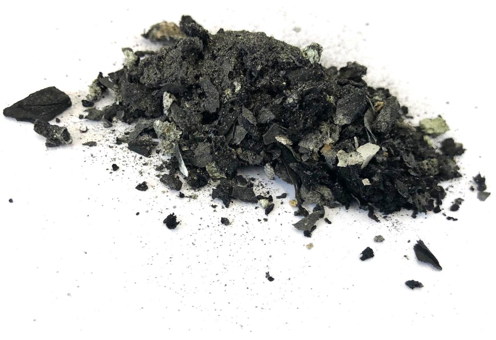
2.1. Samples Characterization

A waste treatment plant in northern Portugal provided the RDF required for this study. Due to the heterogeneity of the RDF, the samples collected were mixed and separated using the coning-quartering method to standardize them for the carbonization process. Then, a carbonization process was carried out to treat the RDF. The RDF sample was carbonized at 400 °C for 30 min, cooled to room temperature, and left exposed to atmospheric moisture for 12 h. The RDF char (RDFc) obtained is shown in Figure 1.

The RDF was composed of a mixture of different materials, with particles of varying diameters. In order to carry out the macro TGA tests, the sample was ground and then sieved through square matrices with a side length of 20 mm. The properties of the original RDF and the RDF char are presented in

Table 1. Proximate and ultimate compositions of the original RDF and the RDF char.

Analysis	RDF	RDF Char
Proximate (%)
Moisture	5.9	3.0
Volatile matter *	85.0	65.1
Ash *	10.4	17.2
Fixed carbon *	4.6	17.7
Ultimate (dry basis %)
Carbon (C)	45.8	59.9
Hydrogen (H)	5.9	5.3
Nitrogen (N)	1.0	1.5
Sulfur (S)	0.1	0.2
Oxygen (O)	36.9	16.0

* Dry basis.

.

Carbonization’s goal is mainly the uniformization of the chemical composition of the RDF via obtaining a product that is considered chemically more stable than the original material. It is also intended that with this process, the pre-treatment of the product reduces the amount of undesired compounds (such as chlorine (Cl)) and, at the same time, increases the carbon and energy content of the sample [9,24]. On the other hand, other characteristics change with the carbonization process, namely, an increase in ashes and fixed carbon and a reduction in the volatile matter and the oxygen content due to the inevitable reactions. Although moisture was eliminated during carbonization at 400 °C, some atmospheric moisture was adsorbed onto the RDFc when this material was equilibrated with the atmosphere at room temperature, thus leading to a moisture content of 3%.

The characterization of the RDFc was carried out according to the following norms: CEN/TS 15414-1 for the moisture content; CEN/TS 15402 for the volatile matter content; CEN/TS 15403 for the ash content; CEN/TS 15407 for the carbon (C), hydrogen (H), and nitrogen (N) contents; and CEN/TS 15408 for the sulfur (S) content.

The fixed carbon and oxygen contents were obtained by default using the values presented in Table 1. The fixed carbon was determined using Equation (1):

$$\%\mathrm{Fixed} \mathrm{Carbon}=100 - \%\mathrm{Volatile} \mathrm{Matter} - \%\mathrm{Ash}$$

(1)

The oxygen content was determined using Equation (2):

$$\%\mathrm{O}=100 - \%\mathrm{C} - \%\mathrm{H} - \%\mathrm{S} - \%\mathrm{N} - \%\mathrm{Ash}$$

(2)

2.2. Experimental Setup and Procedure

The experiment was conducted at the Heat and Fluids Laboratory of the Department of Mechanical Engineering at the University of Minho. A purpose-built macro TGA reactor was designed to perform the tests. The oven (200 mm in diameter and 350 mm in height) was heated up to 1200 °C using a 2 kW electric resistance. To minimize the heat losses, the resistance was surrounded by refractory material along with rock wool. A Nanodec Eurotherm was connected to two type-K thermocouples that were used to control the reactor’s temperature. Inside the reactor was a perforated basket that held the sample. The basket was 62 mm in diameter and 55 mm in height. It was connected by a 3 mm stainless steel cable to a Shinko Denshi AJ-620CE scale to continuously measure the mass of the sample during the test. This scale had an error of 0.01 g and a deviation of 0.001 g. To allow for positioning the basket inside the reactor, a 10 mm slot was machined into the reactor’s rotating lid. A TSI G4043 flow meter was used to control the airflow injected into the reactor. This flow meter was capable of measuring in a range between 0 and 200 L/min with a 2% accuracy and 0.01 L/min resolution. Both the scale and flow meter were connected to a PC with LabView software for data acquisition. The temperature could be set in the Nanodec controller, although there was no possibility to measure it over time.

For the gas analysis, a probe was placed through the reactor lid and followed downstream by four 500 mL Schott bottles to filter the gas. Three of them were filled with water and the last one with cotton. To analyze the gas, a Rapidox 5100 Portable gas analyzer was part of the setup. The gas species read by the equipment, along with their ranges, were as follows:

• CH₄—0–100%—TLD sensor with a 0 to 100% range;
• CO—0–100%—IR sensor with a 0.2% to 100% range;
• H₂—0–100%—TCD sensor with a 10% to 100% range;
• O₂—0–100%—EC O₂ sensor;
• CO₂—0–50%—IR sensor;

where IR—infrared, TCD—thermal conductivity, EC—electrochemical, and TLD—tunable laser diode.

Once the Rapidox internal vacuum pump was not capable of collecting the gas due to the filtering system, an SKC 224-44MTX vacuum pump was used as an auxiliary pump to ensure a proper gas analysis.

A complete scheme of the setup is depicted in Figure 2.

To perform the tests, the reactor was initially pre-heated to the desired temperature. After its stabilization, the basket was introduced into the reactor to set the zero of the scale. Once the zero was well defined, the sample was introduced into the basket, which allowed the heat and air flows to pass through its containing orifices.

Previous tests demonstrated that the injection of air during the residual carbon stage was not as influential as the gas formation process. Taking this into account, the first run was performed without air injection to understand the sample’s behavior with respect to the temperature. Based on this, the fractional conversion parameter ($\mathsf{\propto }$) was calculated with Equation (3) and was set as the reference:

$$\propto =\frac{{\mathrm{m}}_0{ - \mathrm{m}}_{\mathrm{t}}}{{\mathrm{m}}_0{ - \mathrm{m}}_{\mathrm{f}}}$$

(3)

Here, m is the mass of the sample, the subscript 0 stands for the initial mass, the subscript f refers to the mass at the end of the test, and t refers to the mass at the instant t.

The time interval for injecting the air was that corresponding to the period when $\propto$ reached a value of 90% (meaning 90% of the sample’s degradation).

To determine the amount of air to inject into the sample, Equations (4) to (7) were used. Equations (4) to (6) are used to calculate the stoichiometric air in a combustion process, while the amount of air to inject for a desired λ is calculated using Equation (7):

$${\mathrm{C}}_{\mathrm{a}}{\mathrm{H}}_{\mathrm{b}}{\mathrm{O}}_{\mathrm{c}}{\mathrm{N}}_{\mathrm{d}}{\mathrm{S}}_{\mathrm{e}}+x\left({\mathrm{O}}_2+3.76{\mathrm{N}}_2\right) \to { \mathrm{aCO}}_2+\frac{\mathrm{b}}{2}{\mathrm{H}}_2{\mathrm{O}+\mathrm{eSO}}_2{+y\mathrm{N}}_2$$

(4)

where $x$ represents the stoichiometric amount of air for combustion:

$$x=\left(\frac{{\mathrm{m}}_{\mathrm{C}}}{12}\right)+\left(\frac{{\mathrm{m}}_{\mathrm{H}}}{4}\right)-\left(\frac{{\mathrm{m}}_{\mathrm{O}}}{32}\right)+\left(\frac{{\mathrm{m}}_{\mathrm{S}}}{32}\right)$$

(5)

and $y$ represents the number of moles of nitrogen presented on the exhaust gas:

$$y=x\cdot 3.76+\left(\frac{{\mathrm{m}}_{\mathrm{N}}}{28}\right)$$

(6)

$$\mathsf{\lambda }=\frac{\mathrm{Air} \mathrm{inj}.}{\mathrm{Air} \mathrm{stoich}.}$$

(7)

Thus, $\mathsf{\lambda }=1$ for stoichiometric mixtures,$\mathsf{\lambda } < 1$ for rich mixtures (more fuel than air), and $\mathsf{\lambda } > 1$ for poor mixtures (more air than fuel). The total air injected in each experiment was evaluated as the product of the stoichiometric air and λ. The airflow was evaluated by dividing the total air by the duration of the experiment (residence time).

To treat the data from the second test, a second-degree polynomial was written [25], as described by Equation (8):

$$\mathrm{f}\left(x_1, x_2\right){=\mathrm{C}}_0 + {\mathrm{C}}_1 x_1 + {\mathrm{C}}_2 x_2 + {\mathrm{C}}_3 x_1 x_2+ {\mathrm{C}}_4 x_1^2+ {\mathrm{C}}_5 x_2^2$$

(8)

where in this study, $x_1$ was the test temperature and $x_2$ was λ. However, other variables can be used in this equation.

The tests were divided into two groups. In the first iteration, a study was performed at 750 °C by varying λ between 0 and 0.2 and setting the sample’s mass to 5 g, 10 g, and 20 g. The second study consisted of varying the temperature between 700, 800, and 900 °C, along with using three λ values: 0.15, 0.20, and 0.25; both studies were performed to investigate the influence of the variables in the released gas composition.

3. Results and Discussion

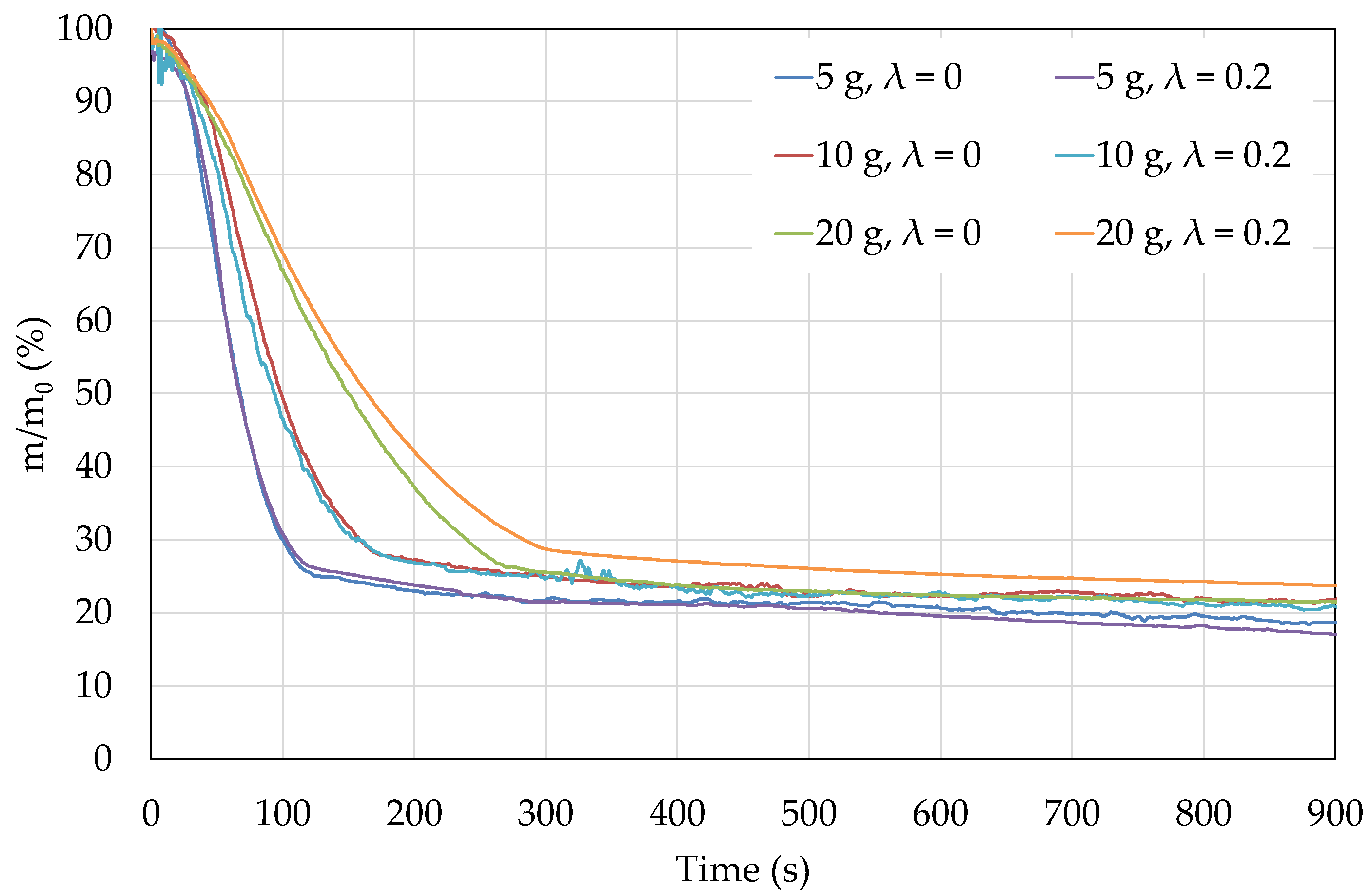
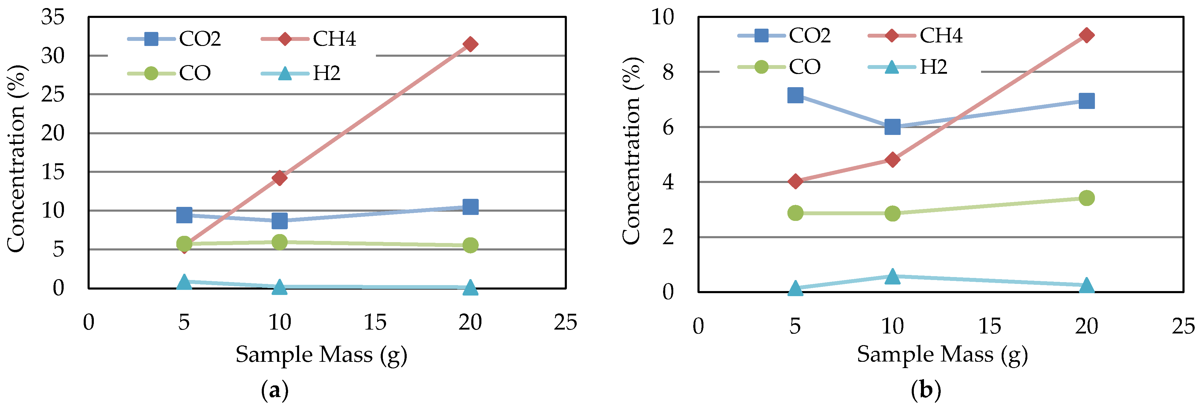
3.1. Influence of the Sample’s Mass and λ

Due to the limitations of the test facility, some initial tests were performed. The tests were mainly concerned with ascertaining whether the amount of sample used influenced the gas composition. In this sense, samples of 5, 10, and 20 g were tested at 750 °C with λ varying between 0 and 0.2. The mass loss of the different tests is depicted in Figure 3.

Regarding the mass loss, the devolatilization stage occurred faster when the sample mass was lower. This phenomenon might have been related to the heat transferred into the sample [26]. The total volume of the RDFc particles introduced into the basket increased with the sample mass; therefore, it required more time to reach the working temperature in its core, thus affecting the devolatilization time.

The final stage of the devolatilization was considered when $\propto$ = 0.9. For all the test conditions, the devolatilization and residual carbon parameters were determined. As can be observed in

Table 2. Characteristics of the devolatilization and residual carbon stages determined at 750 °C for different sample masses and λ values.

λ	Sample (g)	Devolatilization			Residual Carbon
		Time (s)	Mass (%)	Rate (mg/s)	Final Mass (%)	Rate (mg/s)
0	5	114	26.2	33.7	18.6	0.5
	10	168	28.5	42.7	20.9	1.1
	20	264	26.8	56.6	21.4	2.4
0.2	5	113	27.4	33.8	17.0	0.6
	10	171	28.3	42.0	20.4	1.1
	20	298	28.8	48.7	23.6	2.5

, there was a considerable difference in the devolatilization time between the samples, ranging from 112 s with 5 g to 245 s with 20 g when λ = 0 and 151 s with 5 g and 271 s with 20 g when λ = 0.2, with the 10 g results in between. The devolatilization rate also exhibited the same behavior. It was expected that the devolatilization rate increased with the increase in the mass. However, when converting the values, we obtained 0.65, 0.43, and 0.28%/s when λ = 0 and 0.64, 0.42, and 0.24%/s when λ = 0.2 for 5, 10, and 20 g, respectively. This suggests that the lower the mass, the higher the devolatilization rate.

Regarding the behavior during the residual carbon stage, after 900 s of testing, all the samples finished with a similar percentage of mass. The average value for the residual carbon rate for all the samples for both λ values was 0.011%/s. This suggested that in this stage, the reaction rate was independent of the sample mass. Since the sample remained in the oven for a relatively long period (602 to 787 s) after the devolatilization phase, a slow decomposition and partial oxidation of the fixed carbon fraction still occurred, as depicted by the slow mass loss in this period and by the low values of residual carbon measured at the ends of the experiments. The residual carbon values were comparable with the average ash content of the RDF char or slightly higher (1.4% to 6.4%).

The remaining mass after the devolatilization phase and the residual carbon (final mass) increased with the sample mass, confirming the heat and mass transfer limitations that affected both the reaction kinetics and the final equilibrium values. The variation in excess air coefficient from 0 to 0.2 at this temperature did not have a major impact on either of the samples, as can be observed in Figure 3 and Table 2, suggesting that the thermochemical decomposition process at this temperature was less affected by small differences in the amount of oxygen available than by the kinetics of oxygen diffusion through the sample volume.

The amount of gas released was also determined and the results are depicted in Figure 4, where the concentration of each species is given in terms of its amount in the total gas collected, while the remaining mass was O₂ and N₂.

It can be observed that CO, CO₂, and H₂ showed no significant variations with sample size. With the available data, it is possible to affirm that these gases’ behaviors were independent of this parameter. However, the opposite behavior was noticed for CH₄. The concentration of this species increased with the increase in the sample’s mass, reflecting a lower degree of oxidation of the sample decomposition products. The minimum and maximum values obtained for this species were 5.5 and 31.5% for λ = 0 and 4.0 and 9.3% for λ = 0.2, respectively, which are consistent with a higher level of carbon oxidation for a higher oxygen availability.

The change in the concentration between the two λ values agrees with the literature. Thus, λ = 0 (pyrolysis condition) favored the increase the CH₄ production compared with λ = 0.2, which tended to represent a gasification condition with a higher level of carbon oxidation [27].

Nevertheless, the subsequent tests were performed with samples of only 10 g each. The utilization of 20 g samples showed a limitation of the current experimental setup, leading to some obstructions in the gas ducts that emerged after the tests.

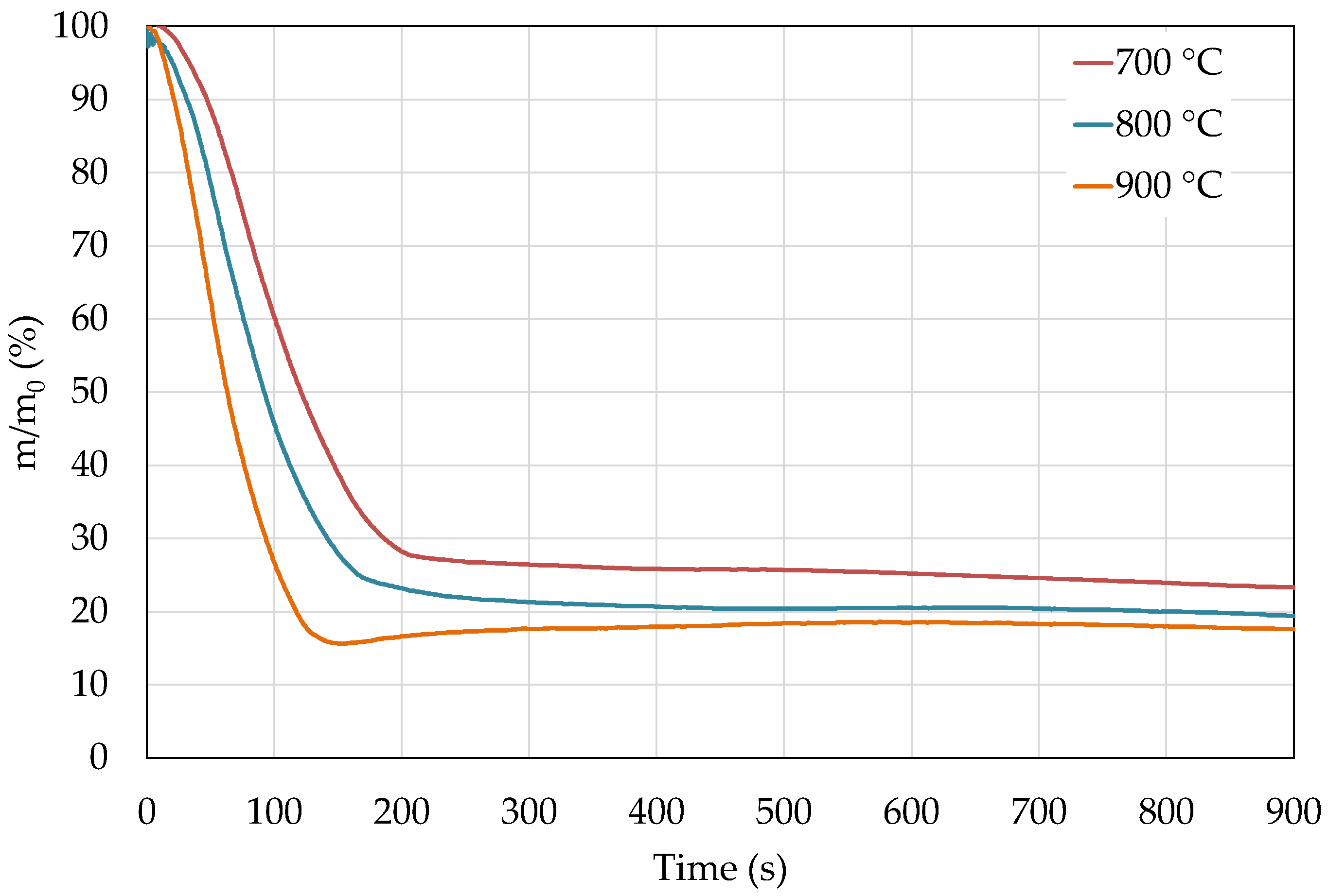
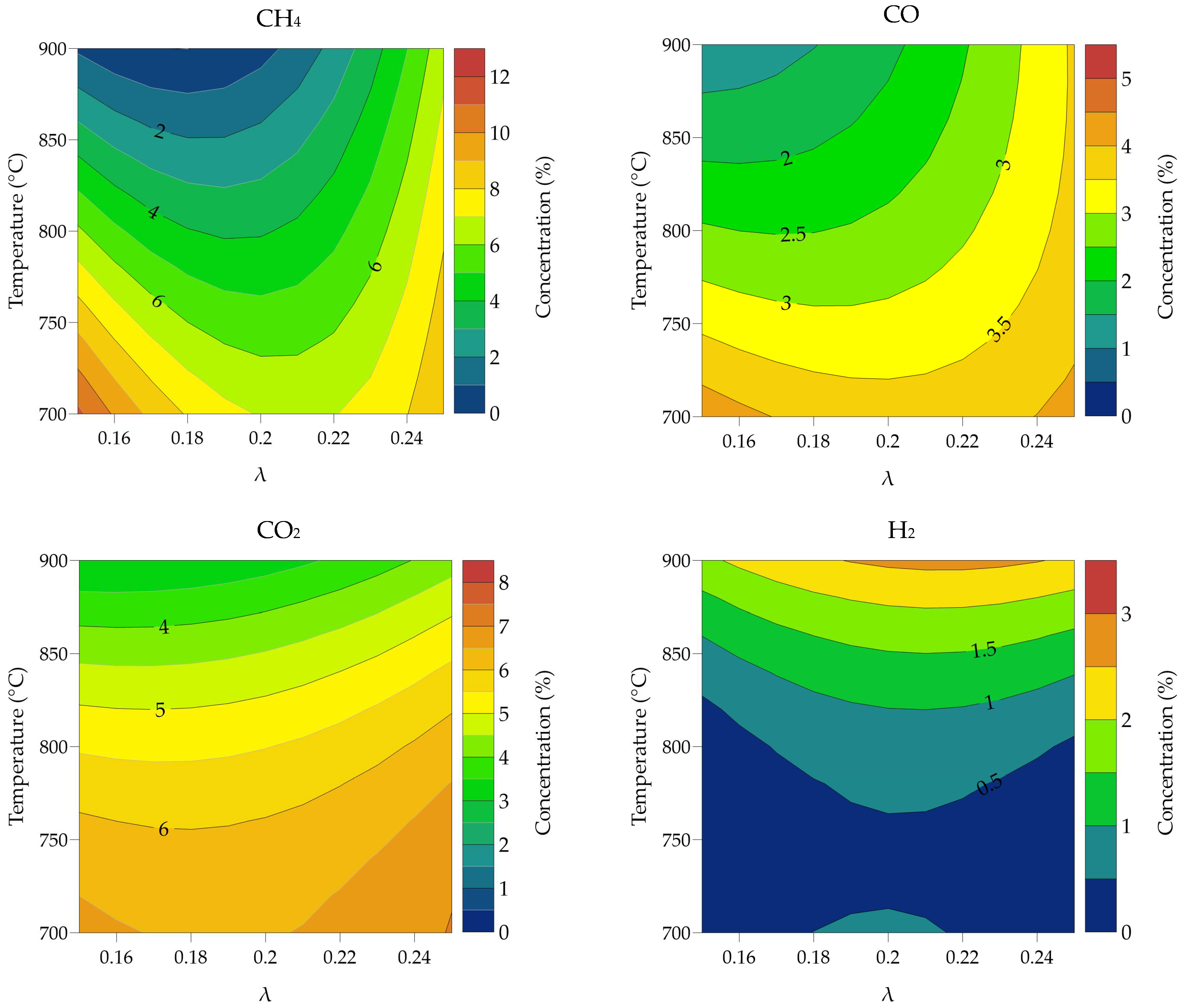
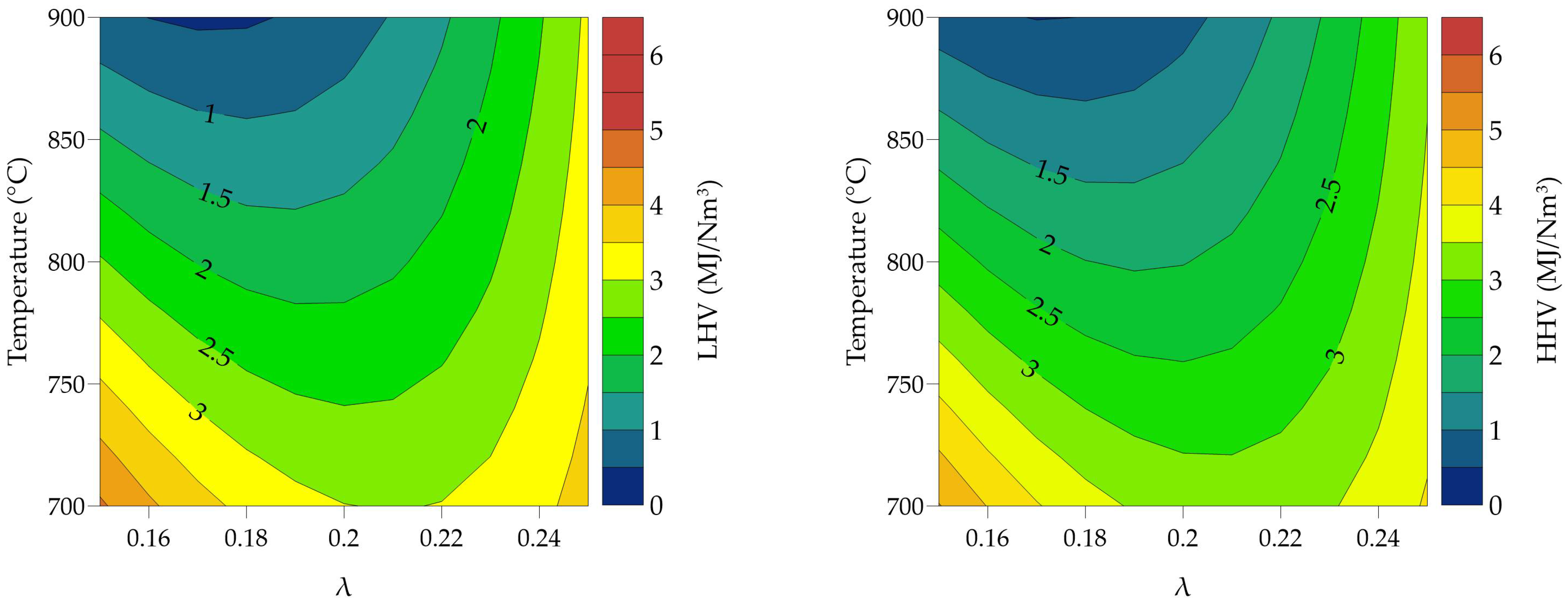
3.2. Influence of the Temperature and λ

It is noticeable in Figure 3 that when samples of 10 g in mass were used, λ had no considerable influence on the mass loss or devolatilization of the sample. For this reason, Figure 5 only depicts the influence of the temperature in the sample with λ = 0.2.

The major fact that stands out from the devolatilization stage was that the increase in temperature decreased the devolatilization time and increased the mass loss of the sample [28,29]. Complementary information is depicted in

Table 3. Characteristics of the devolatilization and residual carbon stage for the sample temperature and λ variation for a 10 g sample.

Temp (°C)	λ	Devolatilization			Residual Carbon
		Time (s)	Mass (%)	Rate (mg/s)	Final Mass (%)	Rate (mg/s)
700	0.15	172	28.3	43.1	20.4	1.1
	0.20	183	30.5	38.2	23.0	1.1
	0.25	181	30.0	39.1	22.3	1.1
800	0.15	145	26.2	52.1	18.1	1.1
	0.20	153	27.3	48.5	19.4	1.1
	0.25	146	25.4	51.6	17.3	1.1
900	0.15	117	25.6	64.2	17.7	1.0
	0.20	103	25.4	72.9	17.4	1.0
	0.25	103	23.4	85.0	14.9	1.2

, where it is observed that the devolatilization time was reduced from 183 s to 103 s by increasing the temperature from 700 °C to 900 °C (both when λ = 0.2). This devolatilization time was also shown in the devolatilization rate of the sample. As can be noticed, the devolatilization rate changed from 38.2 mg/s at 700 °C to 72.9 mg/s at 900 °C (nearly doubling in some cases). Regarding the mass loss of the sample, the difference was not so significant. For the case depicted in Figure 5, after the devolatilization time at 700 °C, the loss was 30.5% of the mass, while at 900 °C, the loss was 25.4%, a difference of only 5%. It is reasonable to consider that within the working range, the temperature mostly influenced the devolatilization stage rather than the mass loss of the sample. This is in accordance with Silva et al. [23] when using the same experimental setup for other samples in different testing conditions.

In the residual carbon stage, the final mass was 23% at 700 °C and 17.4% at 900 °C. This agrees with the results obtained for the residual carbon mass loss rate. As the values obtained for both tests were practically the same (1.1 mg/s), it was observed that the temperature gap remained the same, as their slope was the same. It is important to notice that at this stage, no air was injected. In this sense, the results demonstrate that for this operating range, the temperature did not have a visible influence on the residual carbon degradation. However, Silva et al. [23] demonstrated that for other working parameters, and with some variations in the methodology (injection of air in the residual carbon stage), the response of the sample was distinct. The authors concluded that the presence of air in the residual carbon degradation stage enhanced the thermal loss due to the diffusion of oxygen into the solid biomass particles. As a result, the thermal loss gradient was more evident.

Another fact that can be noticed in Figure 5 is the mass loss variation in the transition between the devolatilization and residual carbon stage at 900 °C. More tests should be performed to acquire further conclusions. However, this phenomenon might have been related to the creation of a recirculation zone in the chamber. Once the cold air entered the oven and as it interacted with the devolatilization gases, a recirculation zone was created, acting in a manner similar to a pressure differential. This pulled the basket downward, which resulted in the dip observed in the figure.

To attain a better perception of the gas concentration dependence on temperature and λ, a multiple linear regression using a second-degree polynomial in two variables was performed. Equation (8) was used and the variables $x_1$ and $x_2$ represented the temperature and λ, respectively. The results are represented as contour plots in Figure 6 for the different gas species and Figure 7 for the heating values of the gases, which were also obtained from the gas analyzer.

Once again, CH₄ was the species that achieved the highest concentration for all tests performed. Its highest and lowest concentrations were 11.1% at 700 °C and 1.3% at 900 °C, respectively, both with λ = 0.15. The gas concentration decreased with the increase in the temperature for a constant λ. However, the behavior for each temperature did not follow a consistent pattern. The CO had a similar trend as the CH₄. Its highest concentration was 4.3% at 700 °C and the lowest was 1.5% at 900 °C, both for λ = 0.2. This was followed by CO, whose concentration also decreased with the increase in temperature when at a constant λ. The concentration of CO₂ suggests that combustion conditions were absent inside the reactor, particularly at 900 °C, as it was the regime with the lowest CO₂ concentration. In contrast to a normal gasifier, this was already expected. A normal gasifier uses the sample as a combustible for the process; in this case, an external source (resistance) produced the required heat to feed the process [30]. For the CO₂, it was possible to obtain 7.5% at 700 °C and 3.2% at 900 °C, both with λ = 0.2. Although it is important to control the concentration of CO₂ in a thermochemical process, its importance is irrelevant in terms of the heating value, as this species does not contain chemical energy, only physical energy, as the temperature of the gas when it leaves the reactor is still high [31]. The H₂ was the species that followed a different pattern, as its concentration increased with the increase in temperature. Wu et al. [32] studied the influence of temperature on hydrogen production and obtained a similar behavior (between 500 and 900 °C). The lowest H₂ concentration was 0.2% at 700 °C with λ = 0.15 and the highest was 2.7 at 900 °C with λ = 0.25.

Regarding the heating value of the gas, this followed a trend similar to that of the more dominant species of gas. Taking this into consideration, it is intuitive that the highest and lowest values for the low heating value (LHV) and higher heating value (HHV) followed the trends of the CH₄ and CO species. In these experiments, it was possible to obtain 4.6 and 5 MJ/Nm³ at 700 °C with λ = 0.15 for the highest values of LHV and HHV, respectively, and 0.9 and 1.0 MJ/Nm³ at 900 °C with λ = 0.15 for the lowest values of LHV and HHV, respectively. It should be noted that the heating values take into account a high percentage of N₂ in its composition. Neglecting this compound will cause these values to increase.

The R² for the equation of each species is given in

Table 4. R² for the multiple linear regressions performed for the gas concentrations.

Parameter	R2
CH4	0.9126
CO2	0.8393
CO	0.8421
H2	0.9331
LHV	0.9034
HHV	0.9027

. The values of R² suggest that the values seen in the graphs could be more precise; however, they are sufficiently trustable to be considered in an analysis.

To acquire some information regarding the gas yield that was possible to obtain,

Table 5. Gas yields, in L/kg, of samples obtained through the variation in the temperature and λ for a 10 g sample.

Temp (°C)	λ	CH4 (L/kg)	CO2 (L/kg)	CO (L/kg)	H2 (L/kg)
700	0.15	78.7	45.6	30.3	1.7
	0.20	51.2	50.2	28.3	1.9
	0.25	53.8	42.2	25.3	2.1
800	0.15	19.7	34.0	11.9	5.4
	0.20	31.7	38.8	19.5	8.6
	0.25	68.3	51.6	30.2	1.3
900	0.15	10.2	26.4	11.4	13.2
	0.20	13.7	24.7	14.0	20.4
	0.25	16.2	26.9	20.0	20.9

depicts the amount of gas per kg of sample for each species.

The determination of this parameter considered the total amount of gas released and the percentage of each species in that same amount. As one can observe, it was possible to obtain almost 79 L of CH₄ at 700 °C with λ = 0.15. This is sufficient to use this gas as a fuel to produce useful energy (heat or electricity). At the same time, one should not neglect the considerable amount of CO₂ released. As it is a gas with no chemical energy, in some cases, its introduction to fuel can reduce the ability of the combustibles to react. However, the literature documents that when correctly used, CO₂ can bring some advantages to a combustion process [33].

4. Conclusions

This paper presents a study in a macro TGA facility of an RDF char in several conditions. In the first iteration, the influence of the sample mass on the gas composition was studied, and in the second stage, the influence of the temperature and λ on the gas composition was studied. This work stands out in the literature as it is one that contemplates the study of an RDF char in a macro TGA facility at a constant temperature and with gas collection. This information will be used to set some working parameters for a gasification facility.

From the first tests, it was possible to conclude that the devolatilization rate was dependent on the sample’s mass, where the rate was higher when the mass of the sample was lower. However, for the residual carbon regime, the sample mass was not so important, as the rate in %/s was the same for all samples. Furthermore, it was shown that between 0 and 0.2, λ had a lower influence on the devolatilization rate, except for the highest mass (20 g). A lower devolatilization rate was noticeable with λ = 0.2, which could be related to the air injected and the volume of the reactor. Regarding the gas composition, the sample’s mass had no influence on the CO, CO₂, and H₂ concentration in the gas. This was tested for two λ values (0 and 0.2), and despite the difference in the concentration between these two conditions, the gas concentration of each species was constant in each test. However, CH₄ showed different behavior. Its concentration increased with the increase in the sample’s mass, suggesting that it was not possible to achieve a stable regime for this species. Despite this, the tests concluded that samples larger than 20 g in mass were required to stabilize CH₄. However, only 10 g could be used for the other tests due to equipment limitations. What stands out is the need for improving the gas collection system to test a sample with more mass until a stable CH₄ regime is achieved and adjust all the results obtained by far.

With a second set of tests, the goal was to simulate a gasification process by leaving the sample in low-air conditions. As the λ for 10 g samples had no influence on the devolatilization or residual carbon rate, only temperature was considered. The tests were performed at temperatures of 700, 800, and 900 °C and λ values of 0.15, 0.20, and 0.25. In this case, the temperature showed a major influence on the devolatilization rate of the sample. However, it did not create an impact on the residual carbon combustion. Regarding the gas released, the results showed that the CH₄, CO, and CO₂ followed the same trend of decreasing their concentration with the increase in temperature, and the opposite occurred for H₂ (increased concentration with increased temperature). The same trend was achieved for the calorific value, as these parameters depend mostly on the gas with the highest concentration (CH₄). As the increase in H₂ with the temperature was not sufficient to balance the reduction in CH₄ and CO at the highest temperatures, the heating value decreased with increasing temperature.

References

1. Pamungkas, B.; Kurnia, R.; Riani, E. Potential Plastic Waste Input from Citarum River, Indonesia. Aquac. Aquar. Conserv. Legis. 2021, 14, 103–110. Available online: http://www.bioflux.com.ro/aacl (accessed on 26 December 2022).
2. Statistics Canada. Human Activity and the Environment-Sectoion 1: Introduction. 2015. Available online: https://www150.statcan.gc.ca/n1/pub/16-201-x/2012000/part-partie1-eng.htm (accessed on 26 December 2022).
3. European Environmental Agency. Reaching 2030′s Residual Municipal Waste Target—Why Recycling Is not Enough. 2020. Available online: https://www.eea.europa.eu/publications/reaching-2030s-residual-municipal-waste (accessed on 26 December 2022).
4. European Parliament. Answer Given by Mr Sinkevičius on Behalf of the European Commission. 2021. Available online: https://www.europarl.europa.eu/doceo/document/E-9-2020-006700-ASW_EN.html#ref1 (accessed on 26 December 2022).
5. APA-Agência Portuguesa do Ambiente. Relatório Anual Resíduos Urbanos 2019. 2020. Available online: https://apambiente.pt/sites/default/files/_Residuos/Producao_Gestão_Residuos/DadosRU/RARU2019.pdf (accessed on 22 April 2022).
6. Margallo, M.; Aldaco, R.; Bala, A.; Fullana, P.; Irabien, A. Best available techniques in municipal solid waste incineration: State of the art in Spain and Portugal. Chem. Eng. Trans. 2012, 29, 1345–1350. [Google Scholar] [CrossRef]
7. Basu, P. Biomass Gasification, Pyrolysis and Torrefaction-Pratical Design and Theory, 3rd ed.; Academic Press: Cambridge, MA, USA, 2018. [Google Scholar] [CrossRef]
8. Chyang, C.-S.; Han, Y.-L.; Wu, L.-W.; Wan, H.-P.; Lee, H.-T.; Chang, Y.-H. An investigation on pollutant emissions from co-firing of RDF and coal. Waste Manag. 2010, 30, 1334–1340. [Google Scholar] [CrossRef] [PubMed]
9. Nobre, C.; Alves, O.; Longo, A.; Vilarinho, C.; Gonçalves, M. Torrefaction and carbonization of refuse derived fuel: Char characterization and evaluation of gaseous and liquid emissions. Bioresour. Technol. 2019, 285, 121325. [Google Scholar] [CrossRef] [PubMed]
10. Du, S.-W.; Chen, W.-H.; Lucas, J.A. Pretreatment of biomass by torrefaction and carbonization for coal blend used in pulverized coal injection. Bioresour. Technol. 2014, 161, 333–339. [Google Scholar] [CrossRef]
11. Nobre, C.; Vilarinho, C.; Alves, O.; Mendes, B.; Gonçalves, M. Upgrading of refuse derived fuel through torrefaction and carbonization: Evaluation of RDF char fuel properties. Energy 2019, 181, 66–76. [Google Scholar] [CrossRef]
12. Lombardi, L.; Carnevale, E.; Corti, A. A review of technologies and performances of thermal treatment systems for energy recovery from waste. Waste Manag. 2015, 37, 26–44. [Google Scholar] [CrossRef]
13. Kirsanovs, V.; Žandeckis, A.; Blumberga, D.; Veidenbergs, I. The Influence of Process Temperature, Equivalence Ratio and Fuel Moisture Content on Gasification Process: A Review. In Proceedings of the 27th International Conference on Efficiency, Cost, Optimization, Simulation and Environmental Impact of Energy Systems (ECOS 2014): Proceedings, Finland, Turku, 15–19 June 2014; pp. 1046–1060, ISBN 978-1-63439-134-4. [Google Scholar]
14. Jangsawang, W.; Laohalidanond, K.; Kerdsuwan, S. Optimum Equivalence Ratio of Biomass Gasification Process Based on Thermodynamic Equilibrium Model. Energy Procedia 2015, 79, 520–527. [Google Scholar] [CrossRef] [Green Version]
15. Özveren, U.; Kartal, F.; Sezer, S.; Özdoğan, Z.S. Investigation of steam gasification in thermogravimetric analysis by means of evolved gas analysis and machine learning. Energy 2021, 239, 122232. [Google Scholar] [CrossRef]
16. Felix, C.B.; Chen, W.H.; Ubando, A.T.; Park, Y.K.; Lin, K.Y.; Pugazhendh, A.; Nguyen, T.B.; Dong, C.D. A comprehensive review of thermogravimetric analysis (TGA) in lignocellulosic and algal biomass gasification. Chem. Eng. J. 2022, 445, 136730. [Google Scholar] [CrossRef]
17. Puig-Gamero, M.; Sanchez-Silva, L.; Sánchez, P. Olive Waste Valorization Through TGA-MS Gasification: A Diatomaceous Earth Effect. Ind. Eng. Chem. Res. 2021, 60, 7505–7515. [Google Scholar] [CrossRef]
18. Fernandez, A.; Soria, J.; Rodriguez, R.; Baeyens, J.; Mazza, G. Macro-TGA steam-assisted gasification of lignocellulosic wastes. J. Environ. Manag. 2018, 233, 626–635. [Google Scholar] [CrossRef] [PubMed]
19. Wu, S.; Li, Z. Experimental and modeling study on centimeter pine char combustion in fast-heating Macro TGA. Proc. Combust. Inst. 2022. [Google Scholar] [CrossRef]
20. da Silva, J.C.G.; Alves, J.L.F.; Mumbach, G.D.; Andersen, S.L.F.; Moreira, R.D.F.P.M.; Jose, H.J. Torrefaction of low-value agro-industrial wastes using macro-TGA with GC-TCD/FID analysis: Physicochemical characterization, kinetic investigation, and evolution of non-condensable gases. J. Anal. Appl. Pyrolysis 2022, 166, 105607. [Google Scholar] [CrossRef]
21. Meng, A.; Chen, S.; Long, Y.; Zhou, H.; Zhang, Y.; Li, Q. Pyrolysis and gasification of typical components in wastes with macro-TGA. Waste Manag. 2015, 46, 247–256. [Google Scholar] [CrossRef] [PubMed]
22. Zhang, S.; Yu, S.; Li, Q.; Mohamed, B.A.; Zhang, Y.; Zhou, H. Insight into the relationship between CO2 gasification characteristics and char structure of biomass. Biomass-Bioenergy 2022, 163, 106537. [Google Scholar] [CrossRef]
23. Silva, J.; Castro, C.; Teixeira, S.; Teixeira, J. Evaluation of the Gas Emissions during the Thermochemical Conversion of Eucalyptus Woodchips. Processes 2022, 10, 2413. [Google Scholar] [CrossRef]
24. Ge, L.; Zhao, C.; Zuo, M.; Tang, J.; Ye, W.; Wang, X.; Zhang, Y.; Xu, C. Review on the preparation of high value-added carbon materials from biomass. J. Anal. Appl. Pyrolysis 2022, 168, 105747. [Google Scholar] [CrossRef]
25. Wortman, K. Polynomials in Two Variables. 2022. Available online: https://www.math.utah.edu/~wortman/1060text-pitv.pdf (accessed on 28 December 2022).
26. Daouk, E.; van de Steene, L.; Paviet, F.; Salvador, S. Oxidative pyrolysis of a large wood particle: Effects of oxygen concentration and of particle size. Chem. Eng. Trans. 2014, 37, 73–78. [Google Scholar] [CrossRef]
27. Akhtar, A.; Krepl, V.; Ivanova, T. A Combined Overview of Combustion, Pyrolysis, and Gasification of Biomass. Energy Fuels 2018, 32, 7294–7318. [Google Scholar] [CrossRef]
28. Yan, B.; Zhang, L.; Jin, Y.; Cheng, Y. Effect of Temperature Field on the Coal Devolatilization in a Millisecond Downer Reactor Recommended Citation. 2013. Available online: http://dc.engconfintl.org/cfb10http://dc.engconfintl.org/cfb10/51 (accessed on 2 January 2023).
29. Sudhakar, D.R.; Kolar, A.K. Experimental investigation of the effect of initial fuel particle shape, size and bed temperature on devolatilization of single wood particle in a hot fluidized bed. J. Anal. Appl. Pyrolysis 2011, 92, 239–249. [Google Scholar] [CrossRef]
30. Aydar, E.; Gul, S.; Unlu, N.; Akgun, F.; Livatyali, H. Effect of the type of gasifying agent on gas composition in a bubbling fluidized bed reactor. J. Energy Inst. 2014, 87, 35–42. [Google Scholar] [CrossRef]
31. Cengel, Y.A.; Boles, M.A.; Kanoğlu, M. Thermodynamics an Engineering Approach, 9th ed.; McGraw-hill: New York, NY, USA, 2019. [Google Scholar]
32. Wu, M.-H.; Lin, C.-L.; Chiu, C.-M. Influences of temperature arrangement on hydrogen production during two-stage gasification process. Int. J. Hydrogen Energy 2018, 44, 5212–5219. [Google Scholar] [CrossRef]
33. Kim, H.; Choi, J.; Lim, H.; Song, J. Combustion characteristics of liquid carbon dioxide-dried coal at different pressures of CO2–O2 mixture. Energy 2023, 266, 126431. [Google Scholar] [CrossRef]
Figure 1. RDF char produced from a carbonization process at 400 °C under 30 min.
Energies 16 03064 g001
Figure 2. Experimental setup: (1) sample; (2) sample holder; (3) oven; (4) temperature controller; (5) scale; (6) flow meter; (7) compressed air; (8) cleaning filters; (9) vacuum pump; (10) gas analyzer; (11) data acquisition.
Energies 16 03064 g002
Figure 3. Influence of the sample’s mass and λ value in the mass loss of the RDFc at 750 °C.
Energies 16 03064 g003
Figure 4. Gas composition from the samples: (a) λ = 0; (b) λ = 0.2.
Energies 16 03064 g004
Figure 5. Influence of the temperature on the mass loss of the RDFc for λ = 0.2.
Energies 16 03064 g005
Figure 6. Variation in the gas composition of each species for all tests; multiple linear regression with a second-degree polynomial function was used.
Energies 16 03064 g006
Figure 7. Variation in the heating value for all tests; multiple linear regression with a second-degree polynomial function was used.
Energies 16 03064 g007