Article

Mixed-Mode Ventilation Based on Adjustable Air Velocity for Energy Benefits in Residential Buildings

1
The College of Architecture and Environment, Sichuan University, Chengdu 610207, China
2
The College of Architecture and Urban Planning, Tongji University, Shanghai 200092, China
*
Authors to whom correspondence should be addressed.
Energies 2023, 16(6), 2746; https://doi.org/10.3390/en16062746
Submission received: 6 February 2023 / Revised: 3 March 2023 / Accepted: 13 March 2023 / Published: 15 March 2023

Abstract

:
Energy efficiency and air quality in residential buildings have aroused intensive interest. Generally speaking, the heating, ventilation and air conditioning (HVAC) system is widely used to regulate indoor environmental spaces. Meanwhile, mixed-mode ventilation has been proven to reduce energy consumption and introduce fresh air effectively. This study aims to discuss the correlations between air velocity, temperature and indoor thermal comfort and establish corresponding statistical models based on the ASHRAE_db II database and the Predicted Mean Vote (PMV). On this basis, the air-velocity adjustment strategy, including determining adjustability and establishing adjustable intervals, is optimized based on support vector machine and envelope curve methods. The results show that the recognition accuracy of the adjustability determination model is over 98%, and the air-velocity adjustable interval in the envelope is increased, facilitating control of mixed-mode ventilation. The case shows that interval adjustment increases the sample points by 18.6% (18.1% above 20 °C and 4.5% above 28 °C). Therefore, further research can be supported on improving thermal comfort by air-velocity adjustment to take advantage of the mixed-mode ventilation mode, which is beneficial to building energy efficiency.

1. Introduction

One third of global energy consumption and one quarter of CO2 emissions are caused by buildings [1]. In particular, HVAC systems account for 38% of the building’s energy consumption. Therefore, there is an emergency need to reduce the energy use of HVAC systems. Many efforts have been devoted to this, and programs have focused on finding opportunities to increase energy efficiency [2,3,4,5], including the use of passive ventilation systems as well as mixed-mode ventilation models.
In general, passive system ventilation, e.g., natural ventilation, is insufficient to maintain a comfortable indoor environment all year round because of weather conditions [6]. As a result, a type of ventilation model that combines natural ventilation with mechanical system ventilation has attracted attention, namely the mixed-mode ventilation model. In a mixed-mode ventilation system, natural ventilation is provided by windows or other passive vents. Meanwhile, mechanical ventilation is achieved by mechanical systems providing air distribution and temperature adjustment. Various studies on mixed-mode ventilation have been conducted, demonstrating the validity of mixed-mode ventilation in energy conservation for HVAC [7]. In addition, as enhancing ventilation in a closed indoor environment helps to prevent the spread of COVID-19 [8], mixed-mode ventilation is considered an ideal tool to curb the spread of COVID-19.
Mixed-mode ventilation includes three modes: “change-over”, “concurrent” and “zoned”, which are divided by the Center for the Built Environment [9] according to the natural ventilation (NV) and mechanical ventilation (AC) integration strategy, especially considering the time and space where they work. Research shows that in the transition seasons, the use of a conversion ventilation mode can better meet the requirements of comfort and save energy [10]. This research highlights the importance of the guidance of mixed-mode ventilation because although windows are used as air vents in many buildings, they generally require manual operation by the occupants. The practical problem of the actual situation reflected in the control system shows that dwellers are disturbed by many factors, resulting in uncertainty in using the control system [11]. Baborska-Narożny et al. [12] studied residential bedrooms and user behavior with different ventilation modes, suggesting preferences of user behavior are of great importance to ventilation modes. Arata et al. [13] studied the effects of hybrid ventilation on air conditioning energy consumption and productivity in a spring office using a measurement survey and questionnaire and showed that mixed-mode ventilation increased the male participants’ productivity by approximately 9.1% and saved air conditioning energy. Khoshbakht et al. [14] developed a thermal comfort model treatment based on statistical techniques to conduct a field study of three buildings adopting different mixed ventilation modes. This research shows that adaptive thermal comfort models played a more significant role in semi-manual and manually controlled mixed-mode ventilation buildings. Khadka et al. [15] conducted a field survey of mixed ventilation models in office buildings in Japan. They obtained a higher correlation between comfort and indoor air temperature in mixed-mode ventilation buildings, indicating that the building is more acceptable to the occupants given the thermal environment of mixed-mode ventilation. Although these studies have played a good role in displaying the advantages of mixed-mode ventilation in different ways, few have conducted a statistical analysis of mixed ventilation. They lack a model to judge air velocity and thermal comfort. These can be obtained through machine learning.
Simulation through machine learning methods is a joint research strategy in researching mixed-mode ventilation. Different methods to construct a situation model related to mixed-mode ventilation have been reported: Jeong et al. [16] developed a user-friendly outdoor thermal comfort prediction model using machine learning methods. Zhong et al. [17] used simulated data to fabricate measurements through Bayesian inference and Monte Carlo methods for iterative optimization to predict users’ air conditioning usage. Luo et al. [18] investigated the effect of different machine learning algorithms and data processing methods on prediction accuracy. Wang et al. [19] proposed a learning-based control strategy for chillers/heat pumps in HVAC systems to improve the performance of HVAC systems and provide high-capacity frequency regulation services. Alshoul et al. [20,21,22] used many machine learning methods, including Artificial Neural Networks, Decision Trees and Categorical Boosting et al., to solve the problem of green design and evaluation. These studies show that machine learning has significant advantages in building thermal comfort models, but there need to be more models that focus on temperature and air velocity. Since temperature and air velocity significantly impact thermal comfort and play a significant role in mixed-mode ventilation, it is necessary to build a relevant machine learning model of mixed-mode ventilation.
In summary, mixed-mode ventilation generally benefits energy efficiency and thermal comfort. Although mixed-mode ventilation modes have been extensively studied in the past few years, most studies have treated window modes with 0 or 1 (opening or closing) control or taken particular values [7,23]. In order to make full use of wind resources in combination with comfort, we focus on air-velocity regulation rather than selecting specific values. This work combines wind speed regulation, temperature change and thermal comfort in mixed ventilation. A wind speed determination model based on the envelope curve and the construction method of adjustable wind speed interval under the mixed ventilation mode to ensure comfort is proposed. These statistical results are helpful for the continuity regulation of window opening patterns and conducive to optimizing the daily air conditioning timetable and using enhanced ventilation and natural ventilation in mixed-mode ventilation systems. They further optimize change-over ventilation patterns and save energy.

2. Materials and Methodology

This study presented a simulation model and used it to establish a link between temperature, air velocity and PMV for assessing the continuity regulation of window opening patterns in mixed-mode ventilation. Due to the complexity of the working conditions in real situations, it is not easy to take accurate measurements to build the model directly. Therefore, we take ASHRAE_db II (https://datadryad.org/stash/dataset/ (accessed on 6 February 2023) doi:10.6078/D1F671) data as a sample to simulate realistic data. A relatively ideal simulation model can be obtained considering ASHRAE’s strong representation, comprehensive coverage and large sample size. The model consists of three main components: (1) discuss the relationship between the variables while ensuring comfort; (2) discuss the correlation between air velocity, temperature and PMV in continuous regulation; (3) assess applications and guidance strategies. These main steps were analyzed in the following sessions as in Figure 1:

2.1. ASHRAE Database and Correlation of Variable Relationships

The primary purpose of this step is to discuss the constituent elements that influence ventilation adjustment through windows and their relationships with thermal comfort. In order to accurately capture the correlation between the elements and thermal comfort and obtain an accurate and large amount of data, the ASHRAE database was chosen [24] as the data simulation of the experiment.
The ASHRAE_db II database has 107,583 pieces of data in total, including field research data from 23 countries. The database’s field research data are geographically distributed across five continents with a wide range of locations.
The ASHRAE database has a simple web interface and can be filtered according to various criteria. An interactive web-based thermal comfort visualization tool has also been developed to enable users to explore the data quickly and interactively. This study collected six-dimensional data of the environment and users, including ta, tr, va, RH, Iclo and M, through outdoor and indoor test sites. Based on these six variables, the PMV values can be calculated from the above data and displayed in the ASHRAE_db II database. The data format was as shown in Table 1:
Remark 1.
ta: air temperature measured in the occupied zone (°C, °F); tr: radiant temperature measured in the occupied zone (°C, °F); va: air velocity (m/s, fpm); RH: relative humidity (%); Iclo: intrinsic clothing ensemble insulation of the subject (clo); PMV: predicted mean vote; M: metabolic rate (W/m2).
In order to ensure the quality of data and control the error within a manageable range, the data in the ASHRAE_db II database are preprocessed (outlier screening, etc.). These 30,734 data samples were obtained from 107,583 original data samples after screening and denoising some unreasonable data by removing 76,843 missing data and 6 abnormal data (4 samples with radiation temperature higher than 50 °C and 2 samples with air velocity greater than 6 m/s).
Currently, the primary way of assessing indoor thermal comfort is to use the PMV model proposed by Fanger [25]. PMV is generally defined as a function of six thermal variables associated with air conditions and human behavior, including ta, tr, va, RH, Iclo and M. Among them, air temperature, radiation temperature, relative velocity and air humidity are mainly related to the environment, while clothing combination insulation and metabolic rate are mainly related to the user. In order to achieve universal results in subsequent experiments, two user-related factors, intrinsic clothing ensemble insulation and metabolic rate, were not the focus of attention. Instead, the study focused on the four factors related to the environment.
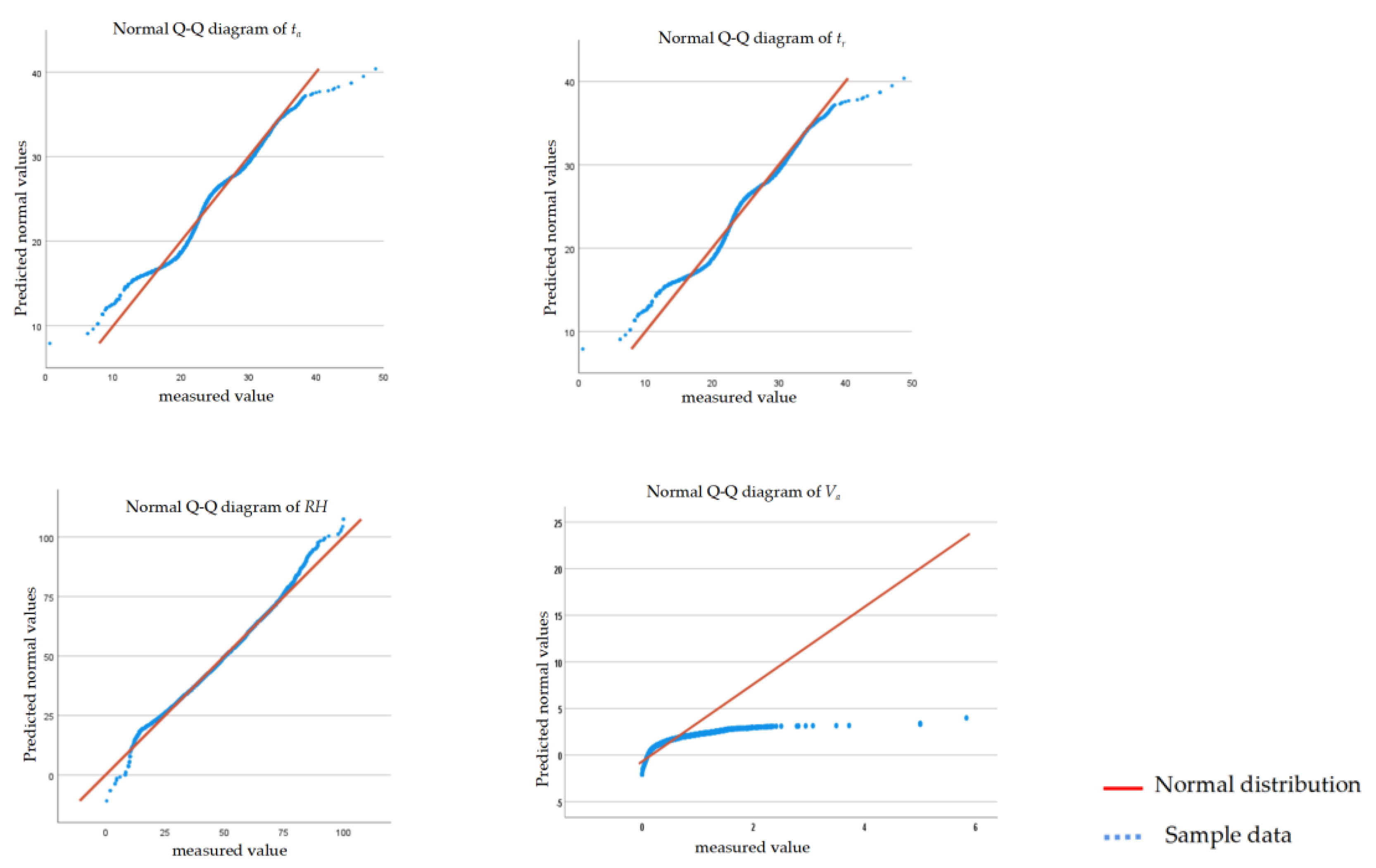
In order to explore the strength of the dependence relationship between the influencing factors, the normality test of each influencing factor was carried out. Table 1 shows that sample va does not present typical distribution characteristics from its skewness and kurtosis values. Meanwhile, samples ta, tr and RH show approximately normal distribution. Furthermore, through the Q-Q diagram verification via SPSS software, it can be seen in Figure 2 as being near a straight line. It was assumed that the relevant influencing factors ta, tr and RH obey a normal distribution.
Further, assuming an approximately linear relationship between the influencing factors ta, tr and RH, analysis was performed using the Pearson correlation coefficient, with the following results.
The scatter Pearson correlation coefficient table (Table 2) revealed the weak statistical significance of the RH linear relationship. Since RH is greatly affected by seasonal variation and the relative position of sampling points, and is not universal, the factor RH will not be considered in this study.
It can be seen from Table 2 that the linear correlation of ta, tr and PMV is vital, so considering the impact of ta and tr on PMV, it can be achieved only by simple linear adjustment. In addition, considering the strong linear correlation between ta and tr, only linear adjustment of ta can achieve the control of PMV. At the same time, the probability distribution of va could be more precise. Therefore, it will be more complex to control PMV by regulating va. In practice, it was more related to user habits, leading to subjective influences. Thus, this study aimed to establish a machine learning model to explore the impact of va on PMV. It will make more effective use of the ambient air-velocity resources and enhance the practical support of PMV by using small cell windows to regulate air-velocity adjustment automatically.

2.2. Air-Velocity Adjustment Strategy Based on Optimal Comfort Intervals

2.2.1. PMV Model

Considering that the PMV indicator represented the thermal sensation of most people in the same environment, Fanger proposed a PMV model for assessing thermal comfort, with a recommended value from −0.5 to +0.5 for PMV, in which the human body generally feels the best thermal comfort.
P M V = ( 0.303 e 0.036 M + 0.0275 ) × L ,
L = M W 0.0014 M ( 34 t a ) 3.96 × 10 8 f c l [ ( t c l + 273 ) 4 ( t r + 273 ) 4 ] f c l h c ( t c l t a 1.73 × 10 5 M ( 5867 P a ) 3.05 × 10 3 × [ 5733 6.99 × ( M W ) p a ] , 0.42 × ( M W 58.15 )
I c l = I c l o × 0.155 ,
f c l = { 1.00 + 1.290 I c l , I c l 0.078 1.05 + 0.645 I c l , I c l > 0.078 ,
h c = { 2.38 ( t c l t a ) 0.25 , 2.38 ( t c l t a ) 0.25 12.1 v a 12.1 v a , 2.38 ( t c l t a ) 0.25 < 12.1 v a ,
t c l = 35.7 0.028 ( M W ) + f c l h c ( t c l t a ) I c l { 3.96 × 10 8 f c l [ ( t c l + 273 ) 4 ( t r + 273 ) 4 ] } ,
p s = { e 16.6536 4030.183 235 + t a , M W > 58.15 0.6105 × e 21.875 × t a 265.5 + t a , M W 58.15 ,
p a = 1000 × R H × p s ,
Remark 2.
L: the thermal load on the human body; W: external work (W/m2); Fcl: factor of clothing area; hc: convective heat transfer coefficient ( W / ( m 2 k ) ); tcl: clothing surface temperature (℃); Icl: the thermal resistance of clothing (clo); pa: the vapour pressure of the surrounding air (Pa). Other symbols in the formula are shown in Section 2.1.
As shown in Equations (1)–(8), in calculating PMV, the computational complexity was high due to the multiple iterations involved in calculating PMV values. At the same time, the enhanced role of natural ventilation in mixed-mode ventilation improved the energy efficiency of residential buildings and increased users’ comfort. However, in practical application, the effectiveness of natural ventilation was often reflected through the highly subjective users’ behavior. Besides, the lack of guidance for comfort control based on PMV values was unconducive to the construction of guidance. Therefore, based on the ASHRAE_db II dataset, air velocity was taken as a sample from 0 to 2 m/s in steps of 0.1 m/s as the air-velocity effect that the window exerted on the indoor test point under theoretical conditions. The relationship between air-velocity adjustment and the interval of optimal comfort PMV values was explored. Then the relationship between air velocity and PMV was constructed by controlling variables within the constraint of PMV∈[−0.5, 0.5] as the guide to adaptively constructing air-velocity adjustment to enhance the effectiveness of natural ventilation.

2.2.2. Determination of Air-Velocity Adjustability

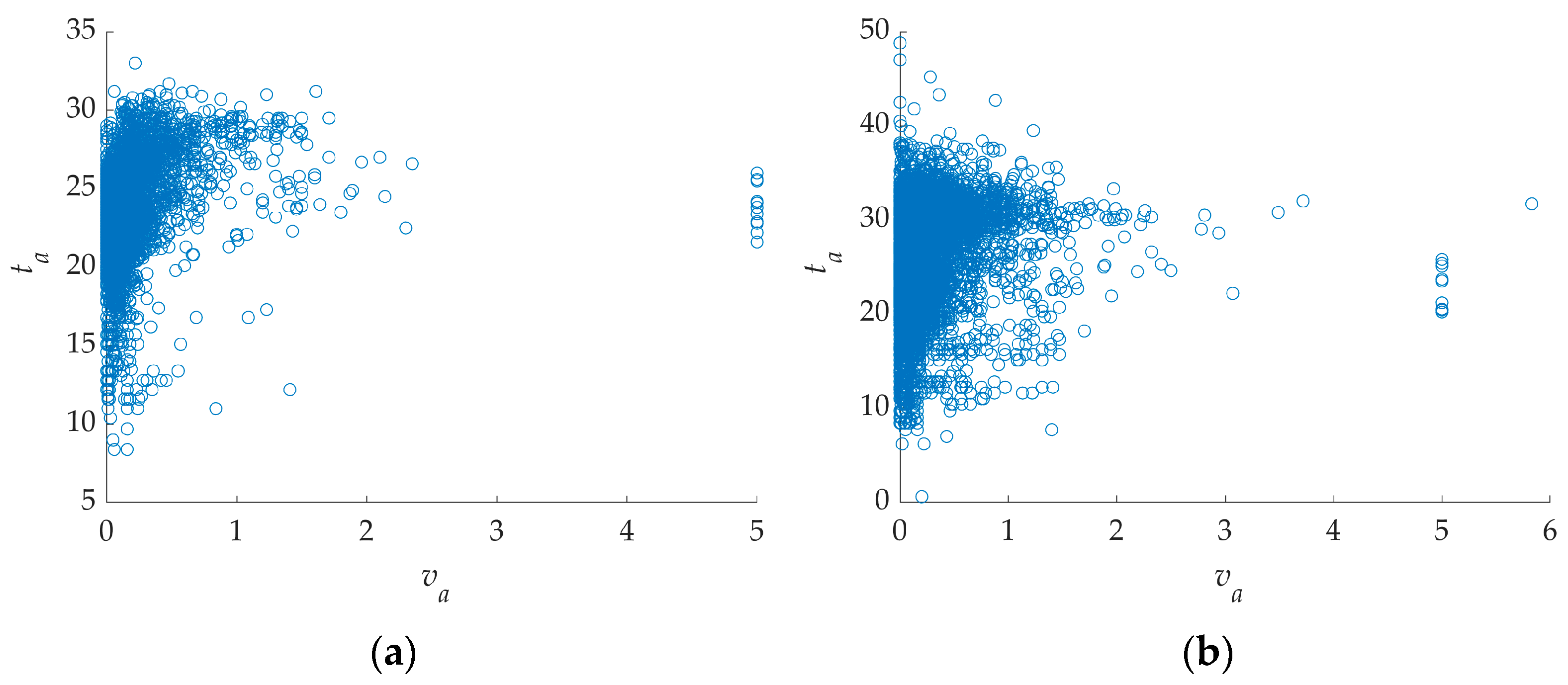
When studying the effect of air velocity on indoor thermal comfort in mixed-mode ventilation in traditional practice, the adjustment of air velocity was reflected in the subjective behavior of the user. In order to make better utilization of the resource of ambient air velocity, the importance of constructing a model that automatically judges the ability of air-velocity adjustment capacity was highlighted. The sample points in Figure 3a had PMV values within the [−0.5, 0.5] comfort interval. In contrast, the sample points in Figure 3b had PMV values that did not fall in the comfort interval ranging from −0.5 to 0.5. It was found that some of the sample points in Figure 3b could be adjusted to bring the PMV values into the comfort zone of [−0.5, 0.5] by adjusting air velocity. Meanwhile, due to the complexity of the iterative operation, it takes a long time for PMV to determine the start-up conditions of mechanical ventilation. In this study, based on the ASHRAE_db II dataset, the air velocity was initially adjusted from 0 to 2 m/s in steps of 0.1 m/s. Then the classification of sample points was judged according to the constraint range of PMV∈[−0.5, 0.5]. Finally, PMV∈[−0.5, 0.5] was regarded as the air-velocity adjustable case, while the others were regarded as non-adjustable. The above determination work utilizes a Support Vector Machine (SVM) as the classifier judgment.
SVM is a classification model proposed by Cortes and Vapnik [26]. A dichotomous discriminant model was adopted owing to its excellent performance in classification tasks, i.e., the category y = {0,1}. It has attracted much academic attention for its excellent performance in classification tasks. The primary classification strategy of SVM is to transform the classification problem into an optimization problem that solves convex quadratic programming and correctly classifies a data set. However, in practical classification problems, the data samples are often linearly indistinguishable, and kernel functions need to be introduced to convert low-dimensional linearly indistinguishable data into linearly divisible problems by mapping them into higher dimensional spaces. The commonly used kernel functions K are polynomial, Gauss and Sigmoid kernel functions, etc.
The study implemented the SVM as Algorithm 1 programmatically using the API interface of the sklearn library package in Python. The API interface was sklearn.svm.SVC, containing the standard parameters C, kernel and gamma. The parameter C was the penalty parameter, the parameter kernel was the kernel function and the parameter gamma was the kernel function coefficient. The grid search algorithm was used to find the optimal parameters of the classification model so that the model could more accurately determine whether the air velocity can be regulated. The specific algorithm was described as follows:
Algorithm 1: Classification algorithm for adjustable air velocity based on optimal comfort interval.
Input: Discrete data from ASHRAE_db II dataset
Output: Recognition accuracy of adjustable air-velocity case
Main framework:
Step1: Data preprocessing (outlier elimination, data smoothing, etc.);
Step2: Select ta, tr, va, RH, Iclo, M forming a six-dimensional feature vector;
Step3: Use SVM for classifying sample points of adjustable air velocity;
Step4: Adopt a confidence level to analyze the experimental results;
Step5: Return recognition accuracy of classification.

2.2.3. Determination of Adjustable Air-Velocity Intervals

The study of air-velocity adjustability determination in Section 2.2.1 found that part of the sample points in the ASHRAE_db II dataset of 30,734 could be adjusted by air velocity to bring the PMV values into the optimal comfort zone [−0.5, 0.5]. Furthermore, as shown in Figure 3a, the adjustable intervals for air velocity showed different distribution patterns as the temperature changed in the sample points where the PMV values belong to [−0.5, 0.5]. The following purpose is to study further the distribution law of sample points with adjustable wind speed and determine the adjustable wind speed interval under temperature. This study adopted an envelope curve [27] to carry out envelope fitting for sample points with adjustable wind speed, and statistical analysis was carried out.
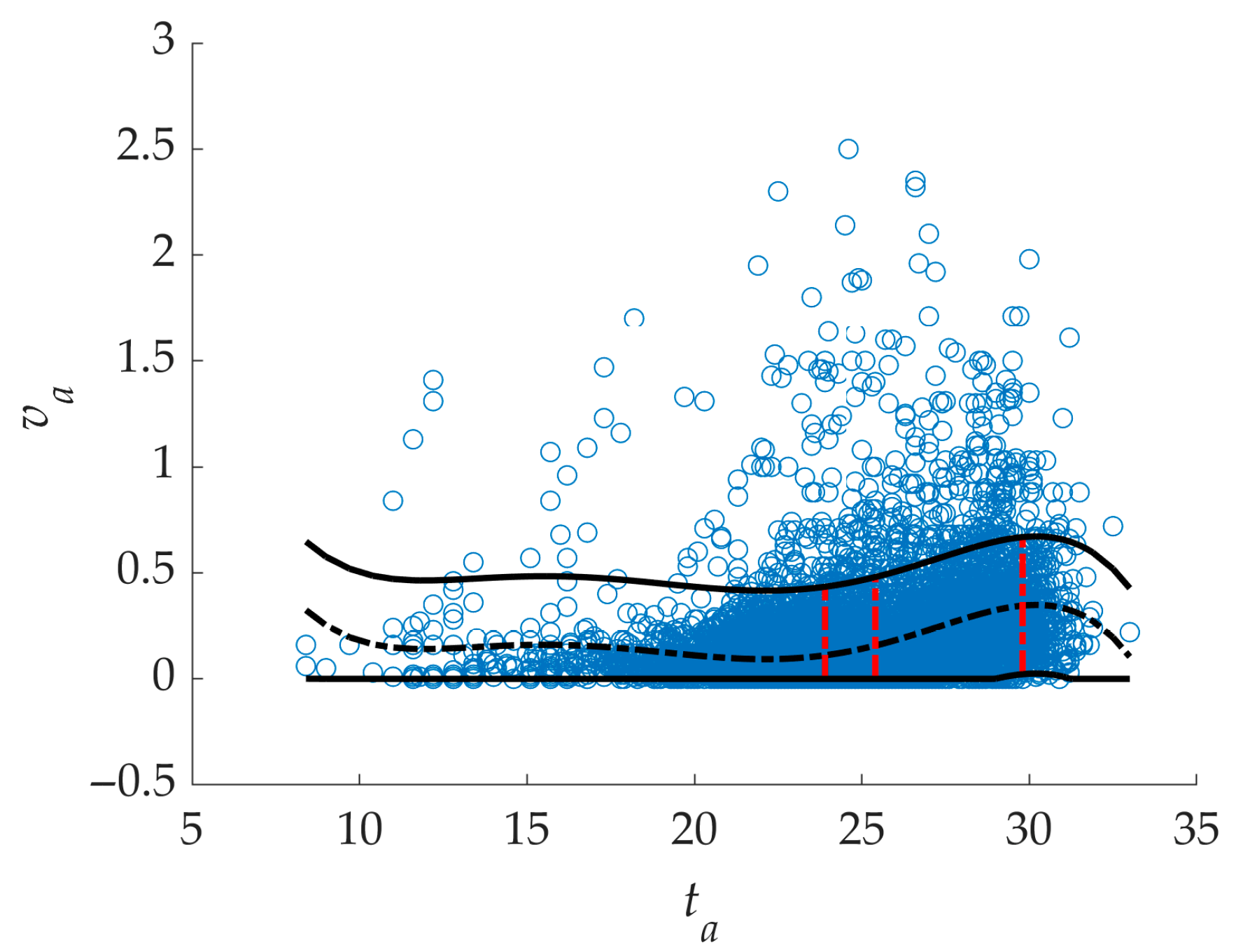
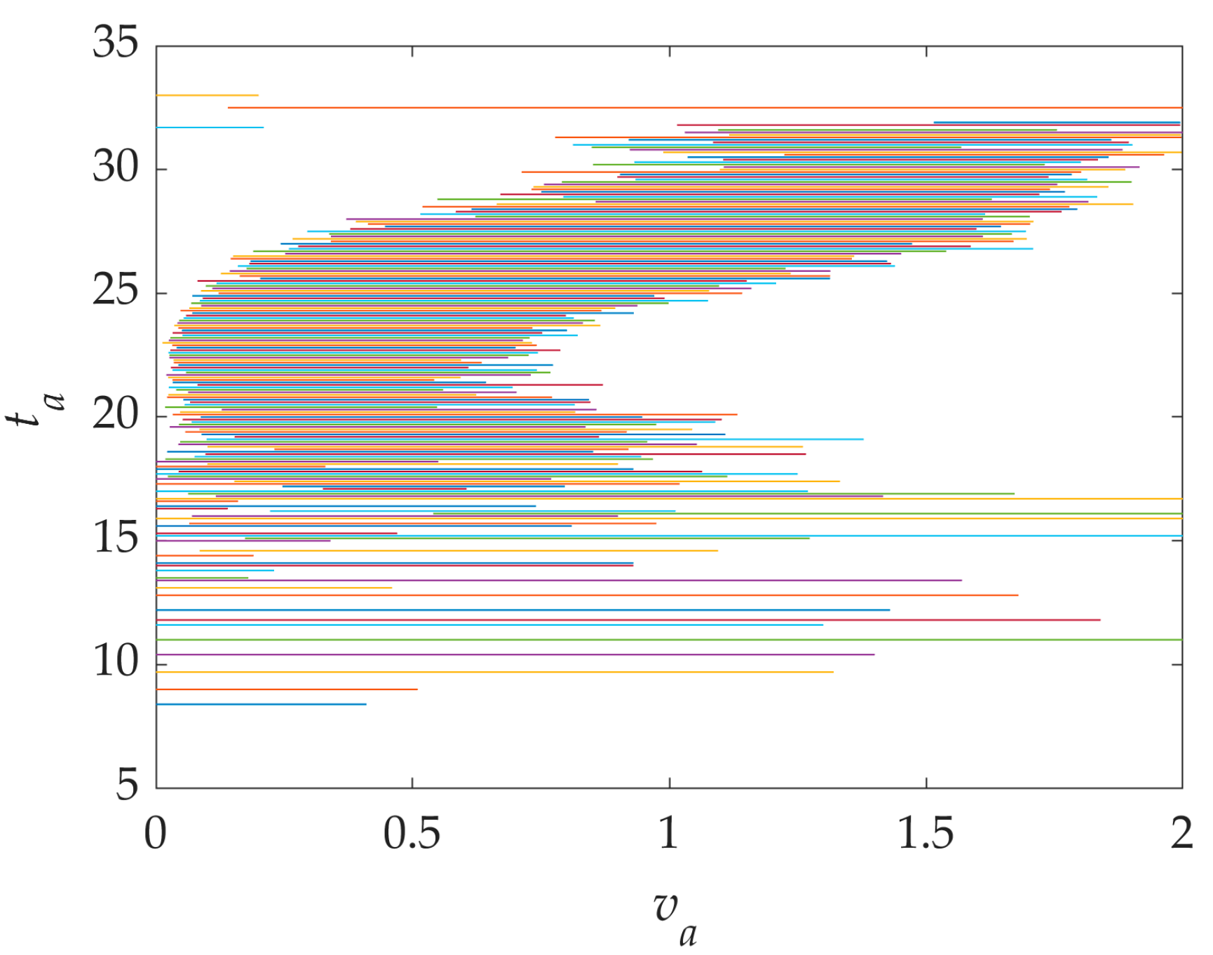
The sample points in Figure 3a were taken as an example; for the scattered data with a PMV value of [−0.5,0.5], the horizontal and vertical coordinates were adjusted to describe them with envelope curves better. The abscissa is the temperature value, and the ordinate is the wind speed value. Moreover, the envelope curves of these data were described, which better shows the adjustable air-velocity intervals at the same temperature. The range of adjustable air-velocity intervals at different temperatures was taken. As shown in Figure 4, the specific calculation process was as follows:
Given the sample point value: (ti*, vi*), i = 1,2,…,n.
Determine the fitted polynomial as:
v = a 5 t 5 + a 4 t 4 + a 3 t 3 + a 2 t 2 + a 1 t + a 0 ,
The residuals, ei, and standard deviations, std, were also calculated as follows:
e i = v i v i , i = 1 , 2 , , n , w h e r e , v i = a 5 t i 5 + a 4 t i 4 + a 3 t i 3 + a 2 t i 2 + a 1 t i + a 0 ,
s t d = 1 n 1 i = 1 n e i 2 ,
An envelope curve with twice the standard deviation of the residuals was determined for the air-velocity adjustable sample points, as shown in Figure 4:
From this, for a determined temperature t ˜ , the adjustment interval for the air velocity was derived as [ max { 0 , v ˜ 2 × s t d } , v ˜ + 2 × s t d ] , where
v ˜ = a 5 t ˜ 5 + a 4 t ˜ 4 + a 3 t ˜ 3 + a 2 t ˜ 2 + a 1 t ˜ + a 0 ,
In addition, from this, the envelope curve and adjustable interval for the air velocity were obtained as shown in Figure 5:

3. Results and Discussions

3.1. Verification of Air-Velocity Adjustability Determination

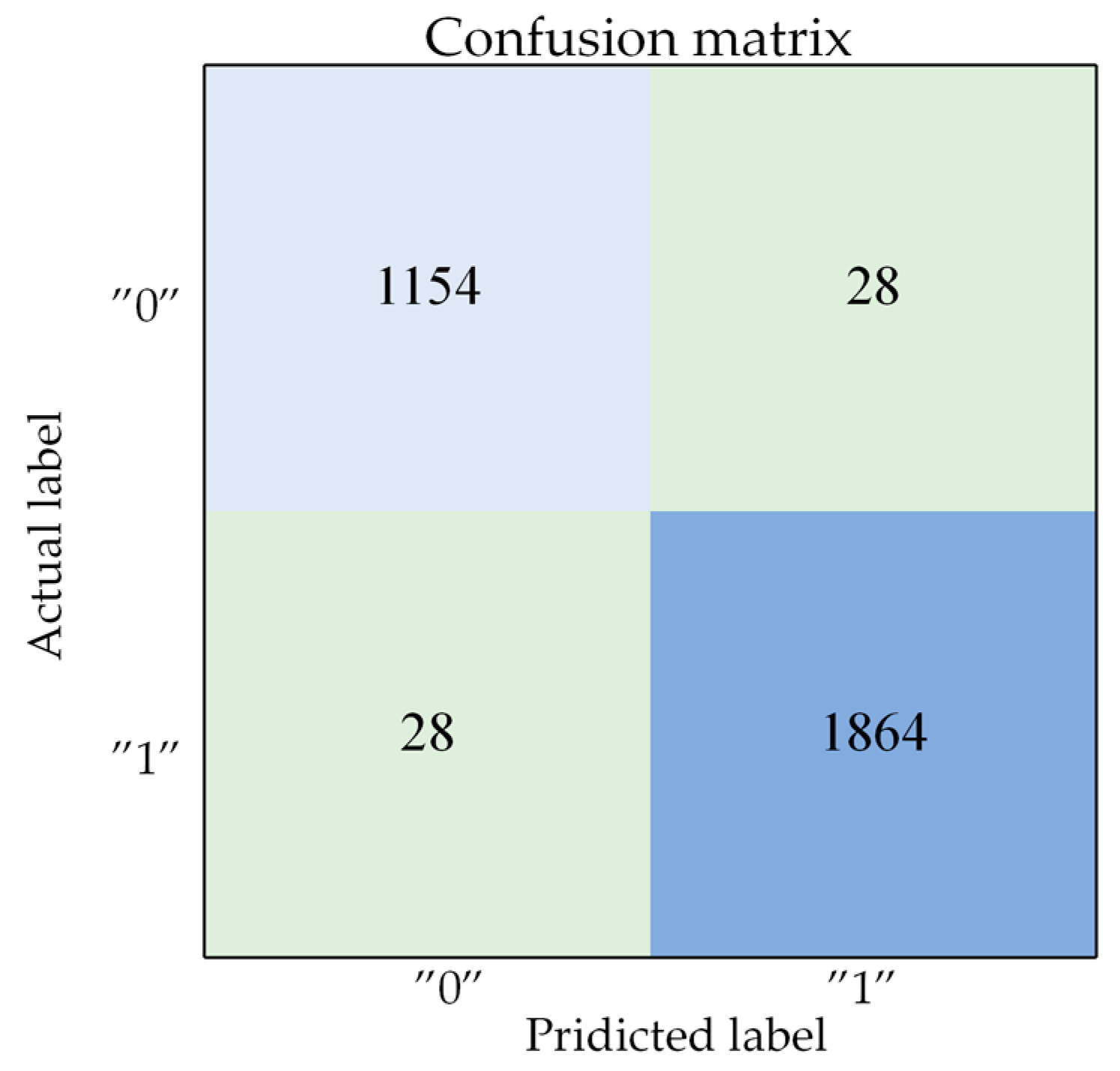
In Section 2.2.2, a machine learning model via an SVM classifier was adopted to construct an air-velocity determination model, which is used for classification determination. The ASHRAE_db II dataset was used, and the number of samples obtained after excluding abnormal data was 30,734. The training set was constructed according to 90% of the sample size, and the test set was 10% of the sample size. According to the PMV value (whether PMV belongs to [−0.5, 0.5]), calculated by taking 0.1 m/s as a step from 0 to 2 m/s as described in Section 2.2.2, the data were labelled according to the constraint range PMV∈ [−0.5, 0.5] (that is, the data PMV∈ [−0.5, 0.5] that can adjust the wind speed are marked as “1”). Since the data are wind speed that cannot be adjusted, PMV∈ [−0.5, 0.5] is marked as “0”. The feature vectors were defined as [ta, tr, va, RH, Iclo, M]. The classifier was a support vector machine (SVM), where the kernel function was taken as a radial basis function with parameters C = 2, degree = 3 and gamma = 1. As shown in Table 3, to prove the construction results’ stability and effectiveness, this study conducted 100 instances of ten-fold cross-validation on the learning results, and the average recognition rate reached more than 98%. The confidence interval of the recognition rate at 95% confidence level is [98.189%, 98.204%]. The confusion matrix is shown in Figure 6. In the confusion matrix, “0” is the adjustable case and “1” is the non-adjustable case. The horizontal coordinate is the forecast label, and the vertical coordinate is the actual label. The confusion matrix represents the number of samples where the predicted labels agree or disagree with the accurate labels.
To validate the rationality of choosing SVM as the classifier for the proposed method, comparative experiments were conducted using K-nearest neighbor (KNN), random forest (RF), AdaBoost, logistic regression (Log), multilayer perception (MLP) and decision tree (DT) methods.
A c c u r a c y = T P + T N T P + T N + F P + F N ,
P r e c i s i o n = T P T P + F P ,
R e c a l l = T P T P + F N
F 1 s c o r e = 2 P r e c i s i o n R e c a l l P r e c i s i o n + R e c a l l
Remark 3.
TP: true positive; FP: true positive; FN: false negative; TN: true negative.
Next, we use an experiment to verify the rationality of choosing a support vector machine as the method classifier in this paper. Comparison experiments were conducted using K-nearest neighbor (KNN), random forest (RF), AdaBoost, logistic regression (Log), multilayer perception (MLP) and decision tree (DT) methods.
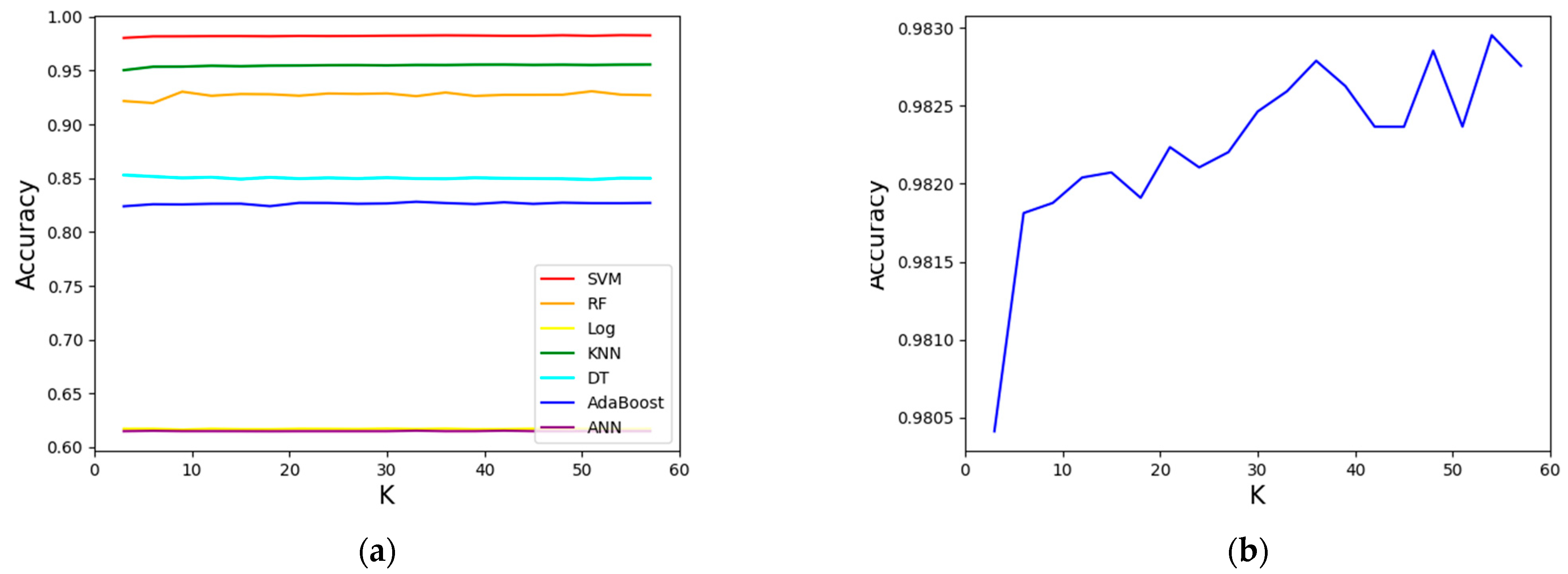
Figure 7 shows the accuracy of the SVM method with different K values in K-fold cross-validation. Despite some fluctuations in the trend line, the classification accuracy remains essentially constant. The classification accuracy tends to stabilize as the K value increases.
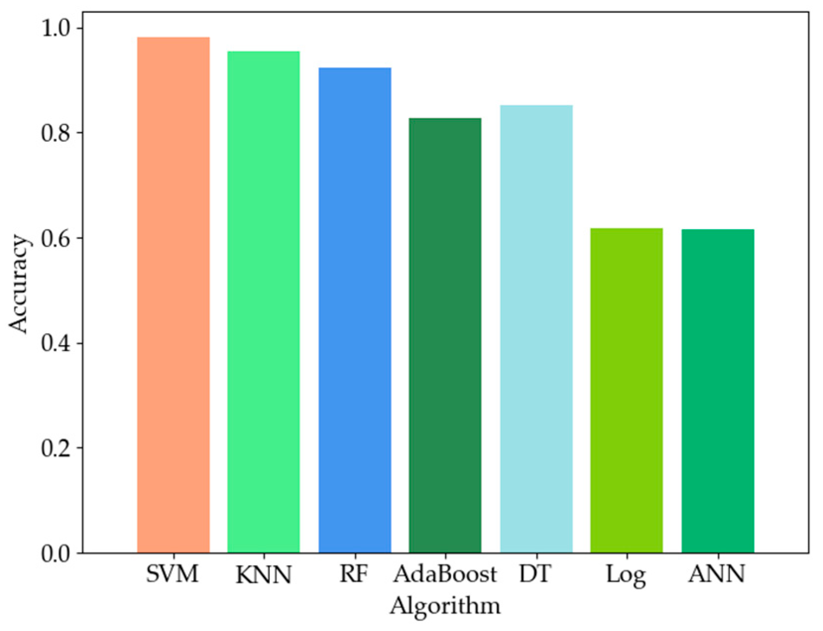
Figure 8 shows the accuracy of seven classifier models. Table 4 gives the seven classifiers’ accuracy, recall, precision and F1-scores. Figure 8 and Table 4 show that the SVM achieves the highest classification accuracy and recall rate. SVM, KNN, RF and ANN have higher precision among the seven models, and SVM has the highest F1-score.
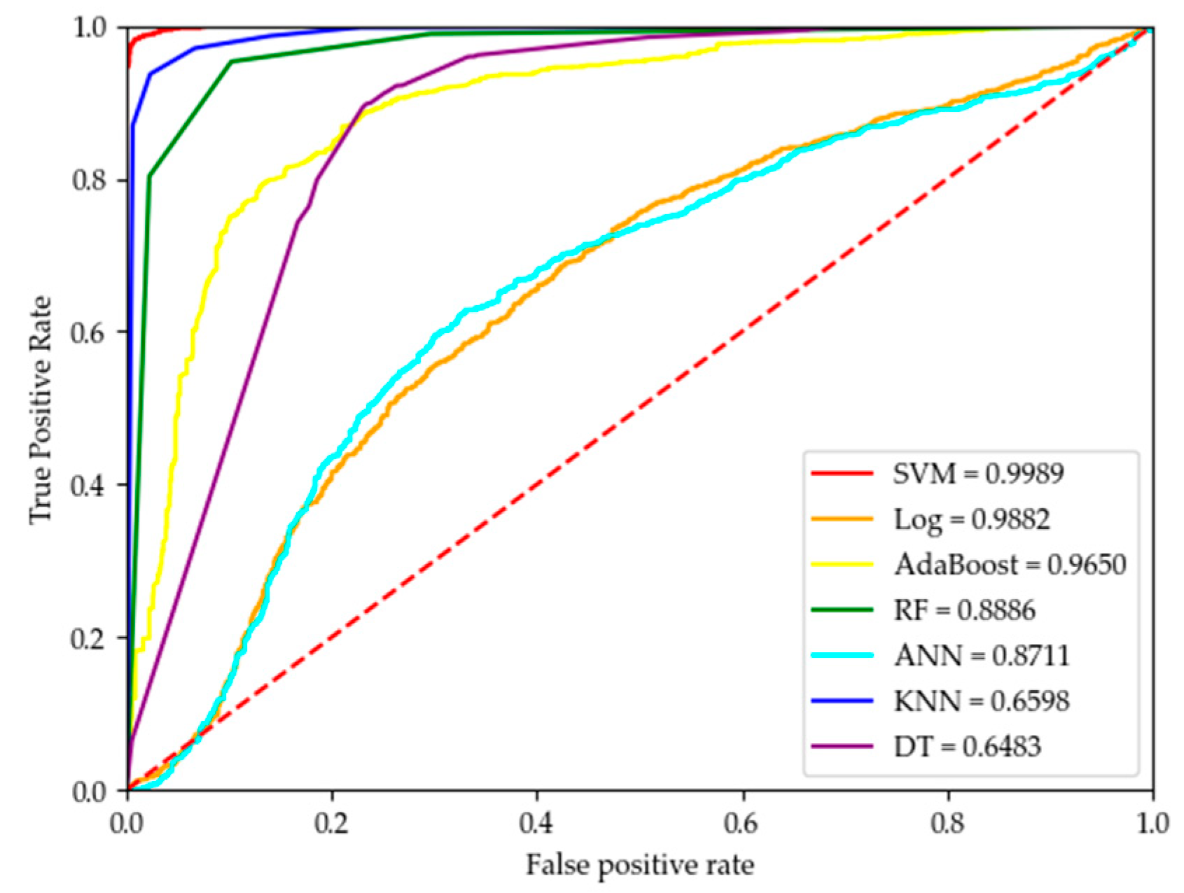
The ROC curves and the corresponding AUC values for the seven classifier models are shown in Figure 9.
As shown in Figure 9, SVM performs the best among the seven classifier models as a robust classifier (AUC = 0.9989). The log models are the second best (AUC = 0.9982). The DT performance could be better than the other six classifier models (AUC = 0.6483).
Compared to the iterative calculation of PMV to verify the comfort performance of determining air velocity, this model reduced the complexity of the determination process. The model facilitates the extraction of parameters of the indoor and outdoor thermal environment through equipment terminals, thus allowing mixed-mode ventilation to determine and select the air-speed setting. The results showed that the sample points meeting the optimum comfort level by air-velocity adjustment were substantially enhanced compared to the original sample points. As shown in Figure 10c, air-velocity adjustment can effectively improve the indoor environment and guide the adaptive enhancement of the effectiveness of natural ventilation in practice.

3.2. Calculation Results and Probabilistic Interpretation of Adjustable Air-Velocity Intervals

As described in Section 2.2.3, the envelope method constructed the correlation between temperature and air velocity that satisfies the optimum comfort interval. Specifically, for the 30,734 original sample points in the ASHRAE_db II dataset, the 18,915 original sample points for which optimal comfort could be met by adjusting the air velocity according to the PMV∈ [−0.5, 0.5] constraint range were selected (air velocity was retained at its original value), resulting in a fifth-order polynomial fit curve of
v = 3.751 × 10 6 t 5 + 0.000374 t 4 0.01432 t 3 + 0.263 t 2 2.322 t + 8.055
The 95% confidence intervals for each of the six coefficients are: [−4.511 × 10⁻⁶, −2.99 × 10⁻⁶], [0.0002929, 0.0004552], [−0.01771, −0.01092], [0.1935, 0.3324], [−3.014, −1.63] and [5.37, 10.74]. For the 18,915 updated sample points where optimum comfort was met by adjusting the air velocity (the updated air-velocity values are taken as random values in the adjustable interval of the adjusted air velocity), the resulting fifth-order polynomial fit curve was:
v = 9.734 × 10 6 t 5 + 0.0009305 t 4 0.03356 t 3 + 0.569 t 2 4.529 t + 14.12
The 95% confidence intervals for each of the six coefficients are: [−1.221 × 10⁻⁵, −7.261 × 10⁻⁶], [6.666 × 10⁻³, 1.194 × 10⁻²], [−4.46 × 10⁻², −2.252 × 10⁻²], [0.3433, 0.7947], [−6.78, −2.278] and [5.39, 22.85]. The envelope curve was obtained by adding/subtracting twice the standard deviation of its residuals from the fitted curve, as shown in Figure 4 and Figure 5 as well as in Figure 11:
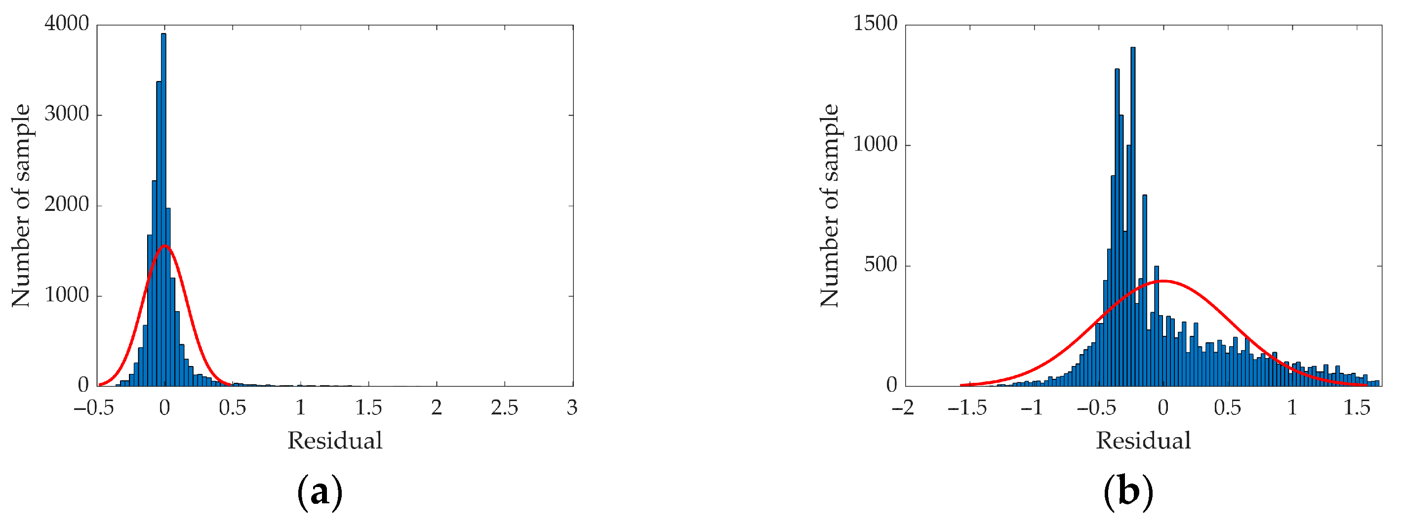
The residuals of the original sample points and the standard deviation of the residuals were calculated to obtain the standard deviation of their residuals: std = 0.1617. Histogram statistics of the residuals were performed, as shown in Figure 12a, to find that the residuals showed an approximately normal distribution. Meanwhile, the residuals and standard deviation were calculated for all updated sample points. The standard deviation of their residuals was: std = 0.5258. Then the histogram statistics were performed on the residuals, as shown in Figure 12b, to find that the residuals also showed an approximately normal distribution. The envelope constructed in this way was relatively reasonable.
Furthermore, an analysis of the statistical significance of the envelope (Figure 5 and Figure 11) leads to the following:
From the endpoints of the quintuple polynomial curve, it was statistically significant that at temperatures above 34 °C, the air-velocity adjustment makes it less likely that the comfort level will meet the condition.
From the upper and lower envelope curves, it can be seen that the adjustable range of air velocity was limited to 0–0.6717 m/s for 95% of cases in the original sample points. Moreover, the specific adjustment interval for air velocity at a fixed temperature t ˜ was derived as [ max { 0 , v ˜ 0.3234 } , min { 2 , v ˜ + 0.3234 } ] . The adjustable range of air velocity was limited to 0–1.0516 m/s for 95% of the cases in the updated sample point, and the specific adjustment interval of air velocity for a given temperature t ˜ was derived as [ max { 0 , v ˜ 0.5258 } , min { 2 , v ˜ + 0.5258 } ] , shown as Figure 11.
Air-velocity adjustment can effectively increase the number of sample points for the optimal comfort level. The case showed that the number of sample points for satisfying the comfort level increased from 13195 to 18915. Simultaneously, the standard deviation value and envelope curve showed that the range of air-velocity adjustment was effectively expanded to meet the optimal comfort and air-velocity efficiency in natural ventilation.
It should be noted that the high proportion of sample points in the 20 °C to 30 °C range and the small number of sample points below 20 °C resulted in distortions in the fitted fifth-order polynomial. This result made it a poor guide below 20 °C, although the fifth-order polynomial satisfied the normality test. Secondly, in the construction of the envelope curve, in order to simplify the calculation, twice the standard deviation of the residual population is used to construct the envelope curve. Indeed, this can be further optimized by seeking, for each temperature value, the local standard deviation of its residuals to form an envelope.

3.3. Guidance Based on Adjustable Air Velocity

As adjustable air velocity has shown advantages in studies to improve the use of wind resources and to select the appropriate air velocity for thermal comfort at different temperatures, the following guidance was given for natural ventilation via air-velocity adjustment in mixed-mode ventilation:
  • According to the conclusions in Section 2.2.2 and Section 3.1, an intelligent terminal allows users to determine whether the comfort level can be improved by air-velocity adjustment and also guides the user in determining the timing of air-velocity adjustment. This conclusion changes the timing of air-velocity adjustment from an uncontrolled and subjective user action to a purposeful user action guided by an intelligent terminal.
By collecting or simulating six environmental and user parameters described in Section 3.1, the intelligent terminal can accurately and efficiently determine whether PMV∈ [−0.5, 0.5] can be achieved by adjusting the air velocity through the SVM classifier. This feature gives the users a guideline for regulating behavior when using natural ventilation in mixed-mode ventilation, thus facilitating better use of air-velocity resources.
2.
According to the conclusions in Section 2.2.3 and Section 3.2, there is a guideline range of air velocity for any temperature between 20 °C and 30 °C (the higher the temperature, the higher the need for air-velocity regulation to meet comfort) when the air velocity is adjustable to meet comfort requirements. Figure 13 gives the average air-velocity interval consisting of the mean of the adjustable air-velocity interval left and correct endpoint values for all given temperatures. This figure clearly guides the air-velocity adjustment strategy at the specified temperature.
3.
As shown in Figure 12 and Figure 13, it is difficult to use air-velocity regulation above 30 °C to make the thermal comfort meet demand, which is a guideline for the temperature determination line of whether to activate the HVAC system for cooling in mixed-mode ventilation. This result means taking HVAC systems for cooling above 30 °C and increasing the use of natural ventilation systems below 30 °C, thus reducing the energy consumption of HVAC systems and influencing the energy efficiency of the building.
4.
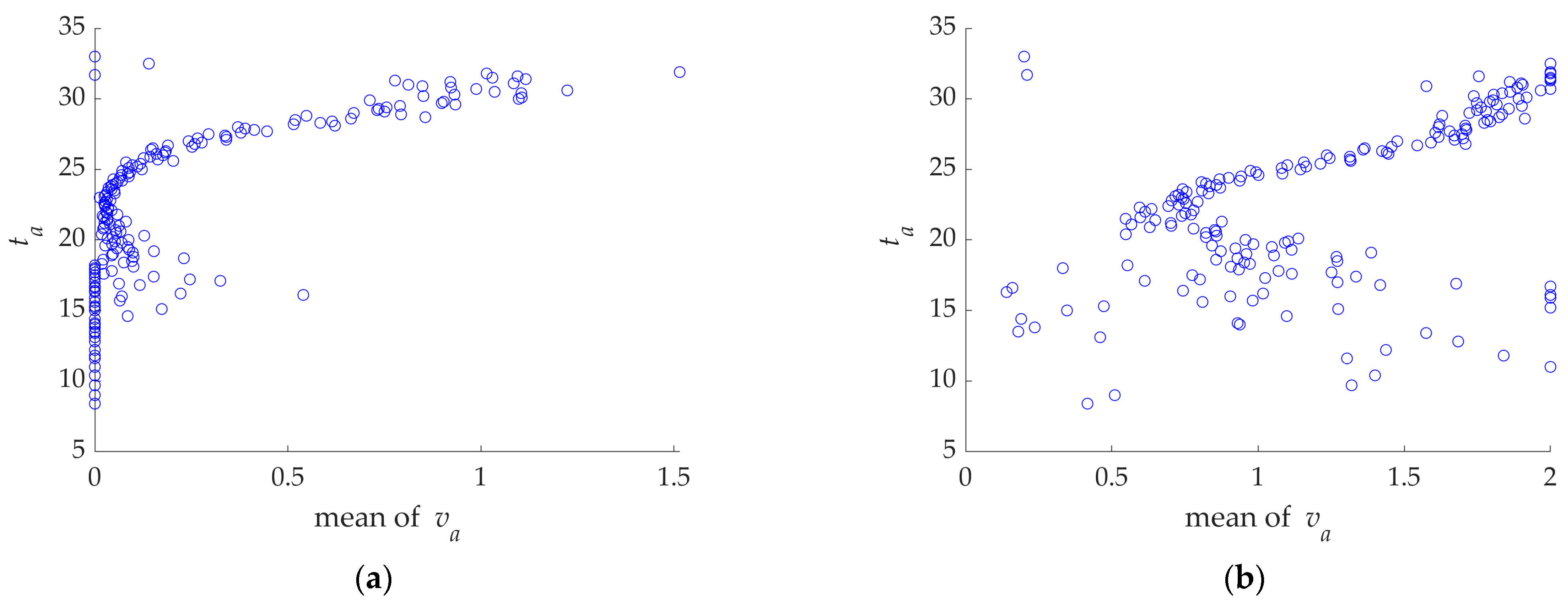
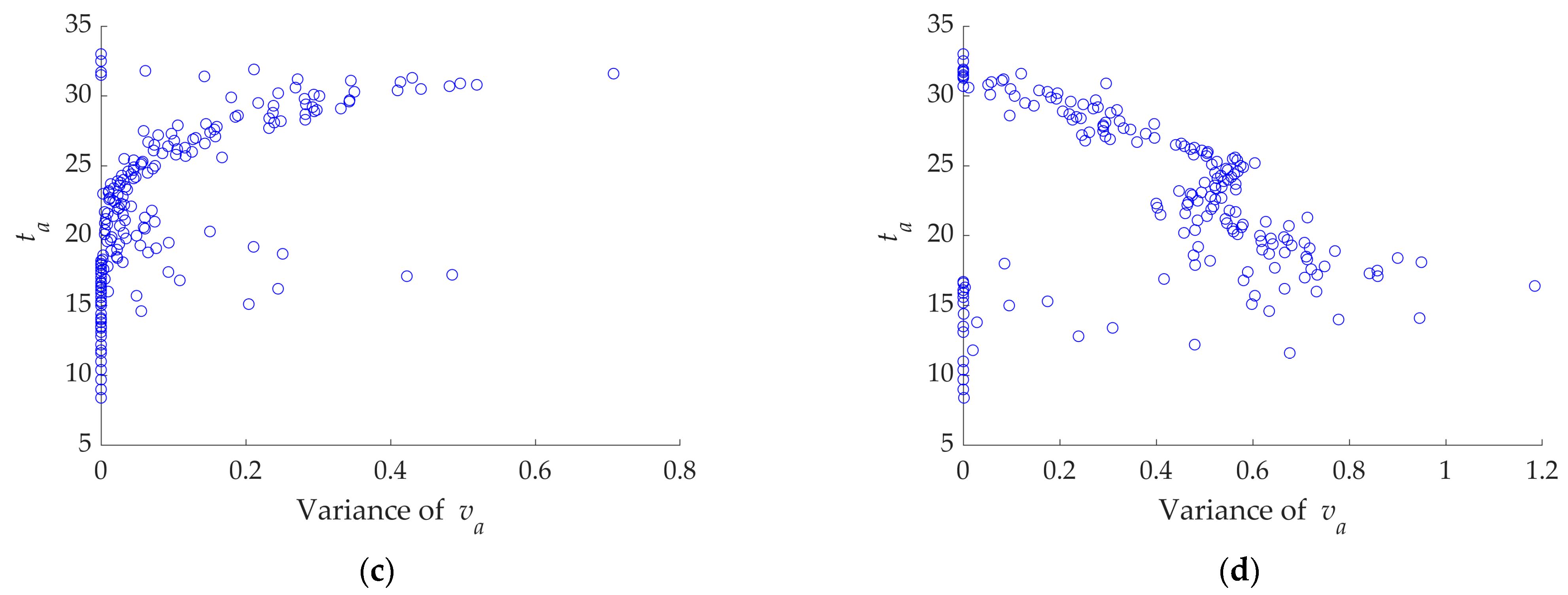
In addition, as shown in Figure 14, when the temperature is below 20 °C, the lower the temperature, the closer the minimum adjustable air velocity is to 0 m/s. In contrast, the maximum adjustable air velocity is influenced by other factors to a greater extent, indicating that the demand for air-velocity regulation to meet the comfort level is not high under low temperatures. When the air temperature is above 25 °C, the higher the air temperature is, the closer the maximum adjustable air velocity is to 2 m/s. In contrast, other factors influence the minimum adjustable air velocity to a greater extent, suggesting a higher demand for air-velocity regulation to meet the comfort level under high-temperature conditions. These results provide a guiding strategy for adjusting air velocity in the mixed-mode ventilation system, i.e., to enhance indoor thermal comfort by increasing or decreasing ventilation to the guidance range of air velocity at a given temperature.

4. Conclusions and Discussions

This study investigates a statistical simulation model corresponding with the SVM model based on the correlation between air velocity, temperature and indoor thermal comfort. A guiding strategy in mixed-mode ventilation is proposed. The results show that continuous ventilation to regulate comfort is useful for mixed-mode ventilation. Compared to the experimental data, the number of cases where the air velocity was adjusted to meet comfort requirements increased by 5720 sample points, proving that the air-velocity resource is under-utilized due to the constraints of the air conditioning system and subjective habitual behavior of people. Therefore, this research proposes a machine learning method (SVM determination model) using the ASHRAE_db II database to obtain a more than 98% recognition rate. This method guides the user’s behavior in adjusting the air velocity in mixed-mode ventilation. On this basis, this study fits sample points with adjustable air velocity by constructing an envelope curve. It gives a statistically significant guideline range of air velocity for each temperature and satisfies the prerequisites for comfort. Thus, air velocity can adjust thermal comfort in mixed-mode ventilation. This research extends the upper limit of the adjustable air velocity range to 30 °C, increasing the number of cases above 20 °C by 5571 and above 28 °C by 1367 using air-velocity adjustment. Determining the upper limit of air-velocity regulation facilitates the optimization of the daily air conditioning timetable and, thus, energy saving. Besides this, the envelope curve facilitates enhanced and natural ventilation in mixed-mode ventilation systems, and both make sense for energy efficiency. This helps to take full advantage of mixed-mode ventilation for indoor thermal comfort adjustment in the summer, thus saving energy.
Despite the contribution of the findings to mixed-mode ventilation and energy efficiency of buildings, this study did not distinguish whether air velocity is given by mechanical structures or natural ventilation. In addition, two variables, temperature and air velocity, were selected for this study, and other factors affecting PMV values need to be further discussed. At the same time, guidance on air velocities below 20 °C requires further research due to fewer sample points and distortions of the envelope curves. Moreover, the PMV model correction for high air velocities and temperatures needs further evaluation. Finally, the research is mainly based on the ASHRAE database for data simulation and analysis, lacking integration with physical models and empirical tests in natural thermal environments. In addition, due to the well-defined low-dimensional features, strong data regularity and low algorithm overhead in this study, the advantages of deep learning have not been reflected. However, with more complex physical models and more multi-factor constraints, it is helpful to consider the deep learning approach for further research.

Author Contributions

Conceptualization, L.S.; methodology, L.S.; software, L.S.; formal analysis, L.Y.; investigation, J.O.; resources, J.O.; writing—original draft preparation, L.S.; writing—review and editing, L.Y.; supervision, L.Y. All authors have read and agreed to the published version of the manuscript.

Funding

This research received no external funding.

Data Availability Statement

The ASHRAE database used in this study can be downloaded at: https://datadryad.org/stash/dataset/ (accessed on 6 February 2023) doi:10.6078/D1F671.

Acknowledgments

In this study, we should thank Mao X.X. for her support with polishing this manuscript and conceptualization discussion and Tang Q.F. and He Q.X. for their support in software and data analysis.

Conflicts of Interest

The authors declare no conflict of interest.

References

  1. González-Torres, M.; Pérez-Lombard, L.; Coronel, J.F.; Maestre, I.R.; Yan, D. A review on buildings energy information: Trends, end-uses, fuels and drivers. Energy Rep. 2022, 8, 626–637. [Google Scholar] [CrossRef]
  2. Vallati, A.; Matteo, M.D.; Fiorini, C.V. Retrofifit proposals for energy efficiency and thermal comfort in historic public buildings: The case of the engineering faculty’s seat of Sapienza University. Energies 2023, 16, 151. [Google Scholar] [CrossRef]
  3. Yang, L.; Liu, X.D.; Qian, F. Optimal configurations of high-rise buildings to maximize solar energy generation efficiency of building-integrated photovoltaic systems. Indoor Built Environ. 2019, 28, 1104–1125. [Google Scholar] [CrossRef]
  4. Yang, L.; Liu, X.D.; Qian, F.; Niu, S.N. Research on the wind environment and air quality of parallel courtyards in a university campus. Sustain. Cities Soc. 2020, 56, 102019. [Google Scholar] [CrossRef]
  5. Mata, O.; Méndez, J.I.; Ponce, P.; Peffer, T.; Meier, A.; Molina, A. Energy savings in buildings based on image depth sensors for human activity recognition. Energies 2023, 16, 1078. [Google Scholar] [CrossRef]
  6. Chen, Y.; Gao, J.; Yang, J.; Berardi, U.; Cui, G. An hour-ahead predictive control strategy for maximizing natural ventilation in passive buildings based on weather forecasting. Appl. Energy 2023, 333, 120613. [Google Scholar] [CrossRef]
  7. Do, H.; Cetin, K.S. Mixed-Mode ventilation in HVAC System for energy and economic benefits in residential buildings. Energies 2022, 15, 4429. [Google Scholar] [CrossRef]
  8. Wang, J.Q.; Huang, J.J.; Feng, Z.B.; Cao, S.J.; Haghighat, F. Occupant-density-detection based energy efficient ventilation system: Prevention of infection transmission. Energy Build. 2021, 240, 110883. [Google Scholar] [CrossRef] [PubMed]
  9. Center for the Built Environment (CBE). About Mixed-Mode. Mixed Mode, Cases Studies and Project Database. University of California, Berkeley. Available online: https://cbe.berkeley.edu/mixedmode/aboutmm.html (accessed on 25 January 2022).
  10. Wanga, L.; Greenberg, S. Window operation and impacts on building energy consumption. Energy Build. 2015, 92, 313–321. [Google Scholar] [CrossRef]
  11. Yao, Y.; Shekhar, D.K. State of the art review on model predictive control (MPC) in heating ventilation and air-conditioning (HVAC) field. Build. Environ. 2021, 200, 107952. [Google Scholar] [CrossRef]
  12. Baborska-Narożny, M.; Kostka, M. Seasonal. Air quality in bedrooms with natural, mechanical or hybrid ventilation systems and varied window opening Behavior-Field measurement results. Energies 2022, 15, 9328. [Google Scholar] [CrossRef]
  13. Arat, S.; Kawakubo, S. Study on productivity of office workers and power consumption of air conditioners in a Mixed-Mode ventilation building during springtime. Build. Environ. 2021, 214, 108923. [Google Scholar] [CrossRef]
  14. Khoshbakht, M.; Gou, Z.H.; Zhang, F. A pilot study of thermal comfort in subtropical Mixed-Mode higher education office buildings with different change-over control strategies. Energy Build. 2019, 196, 194–205. [Google Scholar] [CrossRef]
  15. Khadka, S.; Rijal, H.B.; Amano, K.; Saito, T.; Imagawa, H.; Uno, H.; Genjo, K.; Takata, H.; Tsuzuki, K.; Nakaya, T.; et al. Study on winter comfort temperature in mixed mode and HVAC office buildings in Japan. Energies 2022, 15, 7331. [Google Scholar] [CrossRef]
  16. Jeong, J.; Jeong, J.; Lee, M.; Lee, J.; Chang, S. Data-driven approach to develop prediction model for outdoor thermal comfort using optimized tree-type algorithms. Build. Environ. 2022, 226, 109663. [Google Scholar] [CrossRef]
  17. Zhong, Y.X.; Knefaty, A.D.; Chen, G.X.; Yao, J.; Zheng, R.Y. Forecast of air-conditioning duration in office buildings in summer using machine learning and Bayesian theories. J. Build. Eng. 2022, 61, 105218. [Google Scholar] [CrossRef]
  18. Luo, M.H.; Xie, J.Q.; Yan, Y.C.; Ke, Z.H.; Yu, P.R.; Wang, Z.; Zhang, J.S. Comparing machine learning algorithms in predicting thermal sensation using ASHRAE Comfort Database II. Energy Build. 2020, 210, 109776. [Google Scholar] [CrossRef]
  19. Wang, H.L.; Ding, Z.K.; Tang, R.; Chen, Y.B.; Fan, C.; Wang, J.Y. A machine learning-based control strategy for improved performance of HVAC systems in providing large capacity of frequency regulation service. Appl. Energy 2022, 326, 119962. [Google Scholar] [CrossRef]
  20. Alshboul, O.; Shehadeh, A.; Almasabha, G.; Mamlook, R.E.A.; Almuflflih, A.S. Evaluating the impact of external support on green building construction cost: A hybrid mathematical and machine learning prediction approach. Buildings 2022, 12, 1256. [Google Scholar] [CrossRef]
  21. Alshboul, O.; Shehadeh, A.; Mamlook, R.E.A.; Almasabha, G.; Almuflflih, A.S.; Alghamdi, S.Y. Prediction liquidated damages via ensemble machine learning model: Towards sustainable highway construction projects. Sustainability 2022, 14, 9303. [Google Scholar] [CrossRef]
  22. Alshboul, O.; Almasabha, G.; Shehadeh, A.; Mamlook, R.E.A.; Almuflflih, A.S.; Almakayeel, N. Machine learning-based model for predicting the shear strength of slender reinforced concrete beams without stirrups. Buildings 2022, 12, 1166. [Google Scholar] [CrossRef]
  23. Cook, M.J.; Shukla, Y.; Rawal, R.; Angelopoulos, C.; Caruggi-De-Faria, L.; Loveday, D.; Spentzou, E.; Patel, J. Integrating low energy cooling and ventilation strategies in Indian residences. Build. Cities 2022, 3, 279–296. [Google Scholar] [CrossRef]
  24. Ličina, V.F.; Cheung, T.; Zhang, H.; Dear, R.D.; Parkinson, T.; Arens, E.; Zhou, X. Development of the ASHRAE Global Thermal Comfort Database II. Build. Environ. 2018, 142, 502–512. [Google Scholar] [CrossRef] [Green Version]
  25. Fanger, P.O. Thermal Comfort: Analysis and Application in Environmental Engineering; Danish Technical Press: Copenhagen, Denmark, 1970. [Google Scholar]
  26. Cortes, C.; Vapnik, V. Support-Vector Networks. Mach. Learn. 1995, 20, 273–297. [Google Scholar] [CrossRef]
  27. Bo, P.B. Curve Reconstruction from Unorganized Point Cloud. Master’s Thesis, Shandong University, Jinan, China, 2004. [Google Scholar]
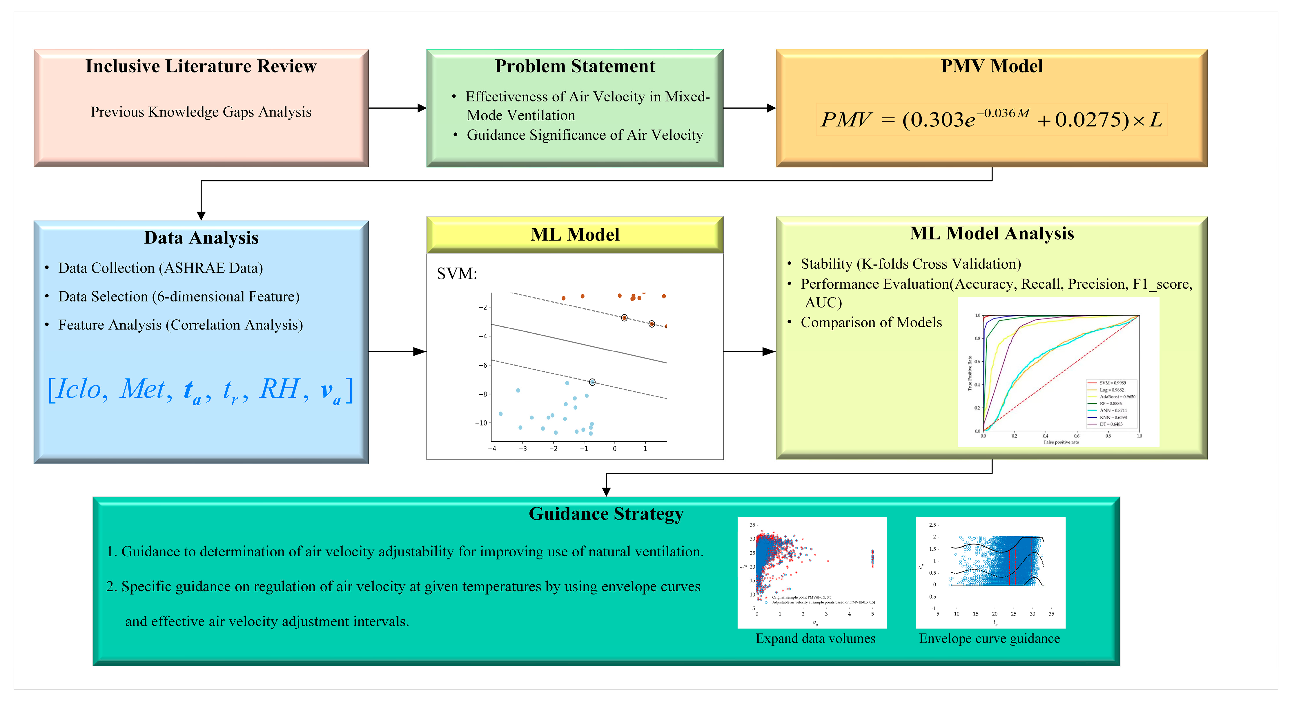
Figure 1. Main framework in the role and method of continuous air velocity adjustment in mixed-mode ventilation.
Energies 16 02746 g001
Figure 2. Normal Q-Q diagram of correlated factors.
Energies 16 02746 g002
Figure 3. Sample points divided via optimum comfort interval; (a) sample points with PMV values fall within [−0.5, 0.5]; (b) sample points with PMV values do not fall within [−0.5, 0.5].
Energies 16 02746 g003
Figure 4. Envelope curves for air-velocity adjustable raw sample points. (The middle dashed line is the fitting curve of data, the upper and lower two lines of the three curves represent the envelope curve).
Energies 16 02746 g004
Figure 5. Adjustable interval for air velocity. The middle dashed line is the fitting curve of data, the upper and lower two lines of the three curves represent the envelope curve. (The lower curve represents the constrained envelope curve with t a 0 ).
Energies 16 02746 g005
Figure 6. Confusion matrix of classification with adjustable and non-adjustable air velocity.
Energies 16 02746 g006
Figure 7. The effects of K-fold method. (a) Comparation between SVM with other methods. (b) K-fold of SVM.
Energies 16 02746 g007
Figure 8. Accuracy of seven classifier models.
Energies 16 02746 g008
Figure 9. ROC curve of seven classifier models.
Energies 16 02746 g009
Figure 10. Adjustable air velocity at sample points based on PMV ∈[−0.5, 0.5]; (a) original sample point PMV∈[−0.5, 0.5]; (b) original sample points PMV∉[−0.5, 0.5], but can be adjusted by air velocity; (c) sample points adjusted by air velocity to meet optimum comfort.
Energies 16 02746 g010
Figure 11. Updating the envelope curve of ta-va sample points when air velocity was adjustable. (a) Air-velocity adjustable update of the envelope curve of the ta-va sample points (no restriction on maximum and minimum air velocity). (b) Air-velocity adjustable update of the envelope curve of the ta-va sample points (limiting the minimum and maximum air velocity to [0, 2] m/s). The middle dashed line is the fitting curve of data, the upper and lower two lines of the three curves represent the envelope curve. The lower curve in (b) represents the constrained envelope curve with air velocity.
Energies 16 02746 g011
Figure 12. Histogram statistics of residuals for adjustable air-velocity sample points. (a) Residual histogram statistics for raw sample points of adjustable air velocity. (b) Residual histogram statistics for updated sample points with adjustable air velocity.
Energies 16 02746 g012
Figure 13. Average interval based on the mean of the left and right endpoint values of air velocity for all air-velocity adjustable intervals. (The color line represents the air velocity adjustment range of each temperature).
Energies 16 02746 g013
Figure 14. Scatter plot of mean and variance based on left and right endpoint values for all air-velocity adjustable intervals. (a) Mean values at the left endpoint. (b) Mean values at the right endpoint. (c) Variance values at the left endpoint. (d) Variance values at the right endpoint.
Energies 16 02746 g014aEnergies 16 02746 g014b
Table 1. Variable description in ASHRAE_db II database.
VariablesUnitIntervalMeanStandard DeviationMedianSkewnessKurtosis
ta°C[0.6, 48.8]24.15 3.96 23.50 0.06 4.44
tr°C[1.2, 49.8]24.47 3.98 23.90 −0.12 4.58
vam/s[0, 5.83]0.16 0.24 0.10 8.44 136.73
RH%[0.5, 100]49.32 14.66 49.80 −0.20 2.85
Icloclo[0.03, 2.87]0.66 0.30 0.60 1.52 6.98
MW/m2[0.65, 6.83]1.22 0.28 1.20 3.05 23.28
PMV [−3, 3]0.03 1.07 −0.01 0.13 3.44
Table 2. Descriptive statistics and correlation analysis of four variables (N = 30734, * p < 0.01).
tatrRHPMV
ta1
tr0.949 *1
RH0.040 *0.075 *1
PMV0.784 *0.786 *0.080 *1
Table 3. The results of classification with adjustable case and non-adjustable case.
CategoryAdjustable CaseNon-Adjustable Case
Mean Recall Accuracy0.985200.97631
Table 4. Performance evaluation of seven classifier models.
AccuracyRecallPrecisionF1-Score
SVM98.16%99.14%97.85%98.49%
KNN95.42%95.81%96.78%96.29%
RF92.72%93.21%95.10%94.14%
BOOST82.82%83.81%89.34%86.49%
DT85.18%83.64%94.42%88.69%
LoG61.72%62.31%95.64%75.46%
ANN61.49%61.53%99.89%76.15%
Disclaimer/Publisher’s Note: The statements, opinions and data contained in all publications are solely those of the individual author(s) and contributor(s) and not of MDPI and/or the editor(s). MDPI and/or the editor(s) disclaim responsibility for any injury to people or property resulting from any ideas, methods, instructions or products referred to in the content.