
Measurement of Gaseous Exhaust Emissions of Light-Duty Vehicles in Preparation for Euro 7: A Comparison of Portable and Laboratory Instrumentation

 , , , and
Abstract
1. Introduction
2. Materials and Methods
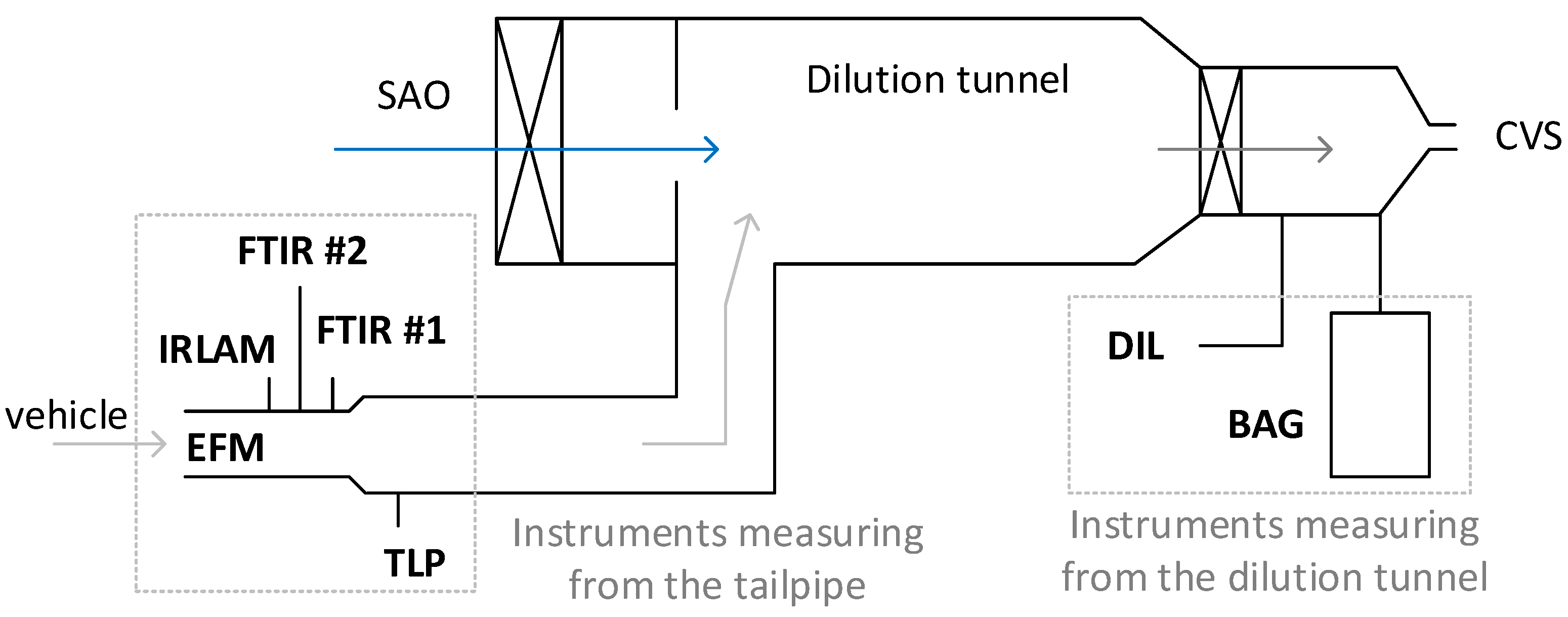
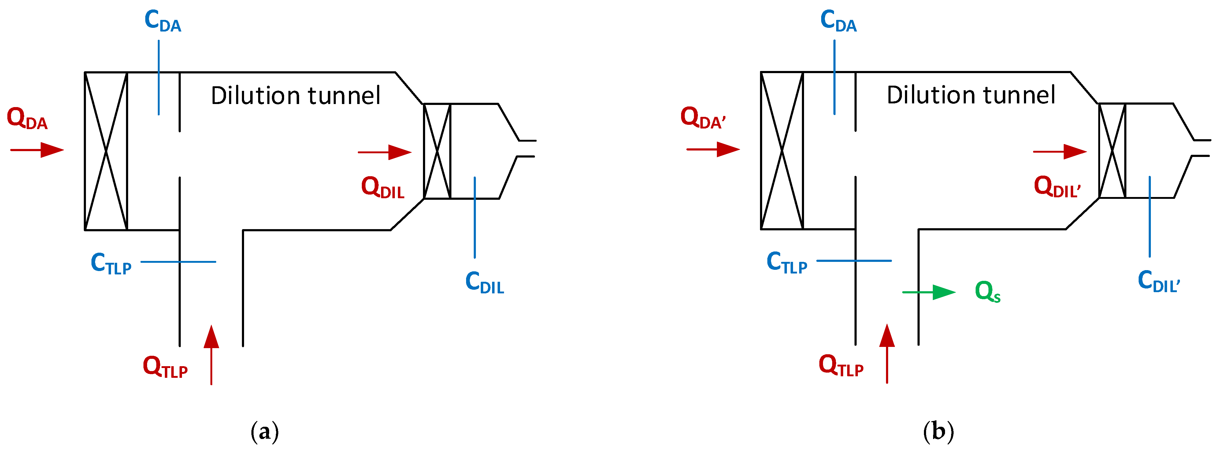
2.1. Setup
2.2. Instrumentation
2.3. Vehicles and Fuels
2.4. Protocol
2.5. Calculations
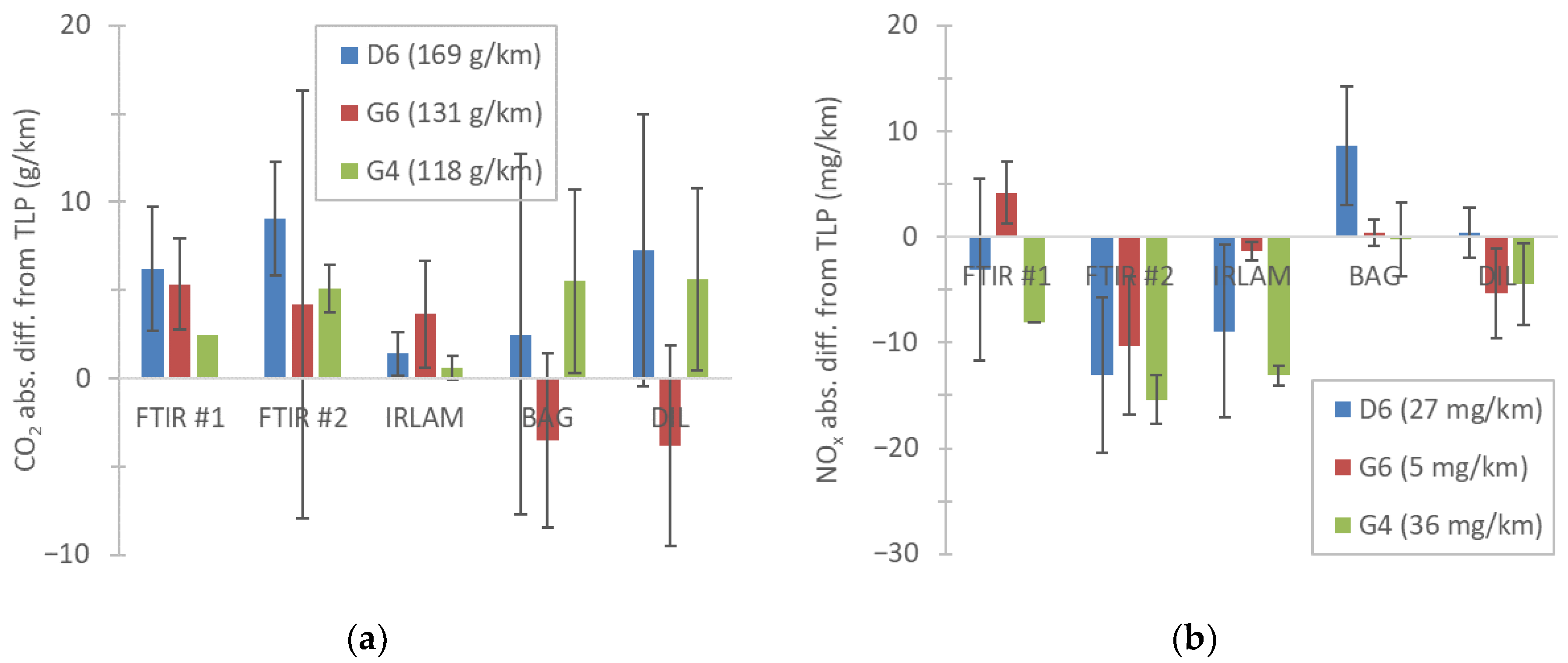
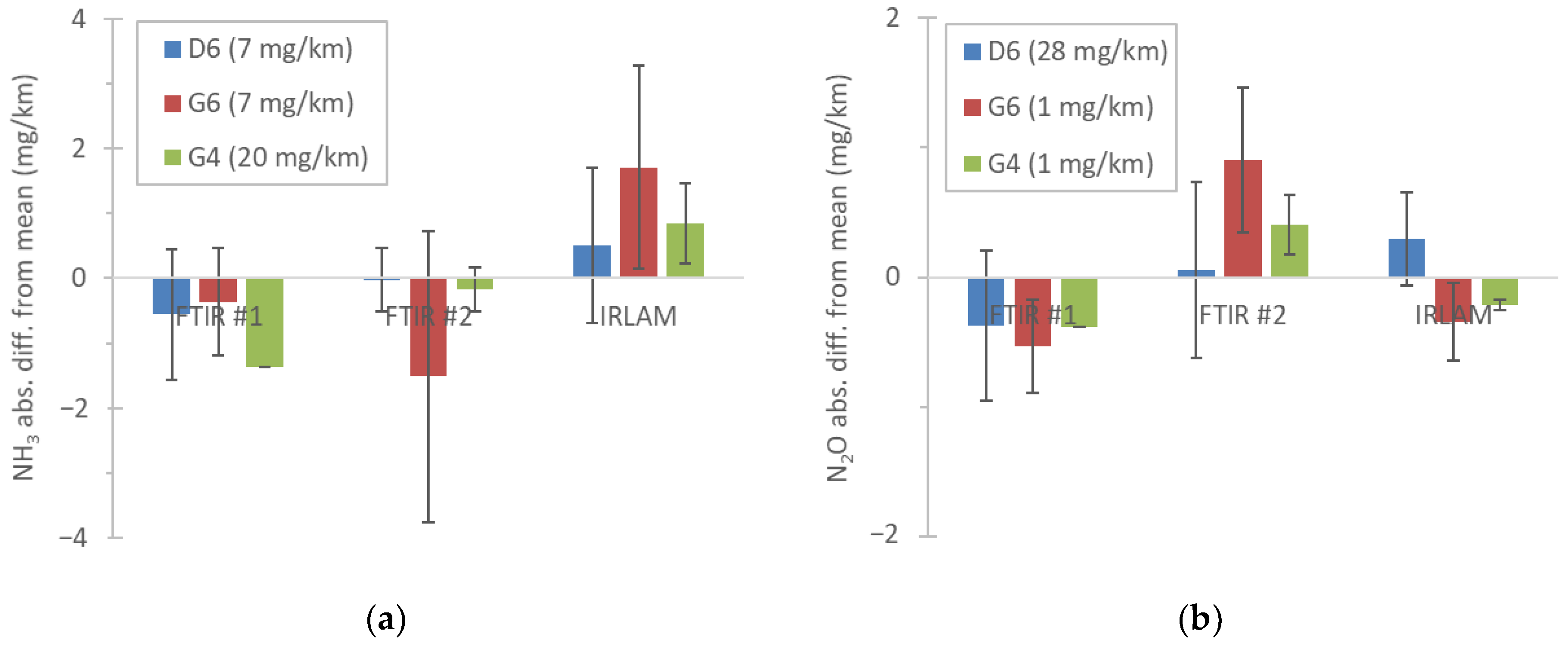
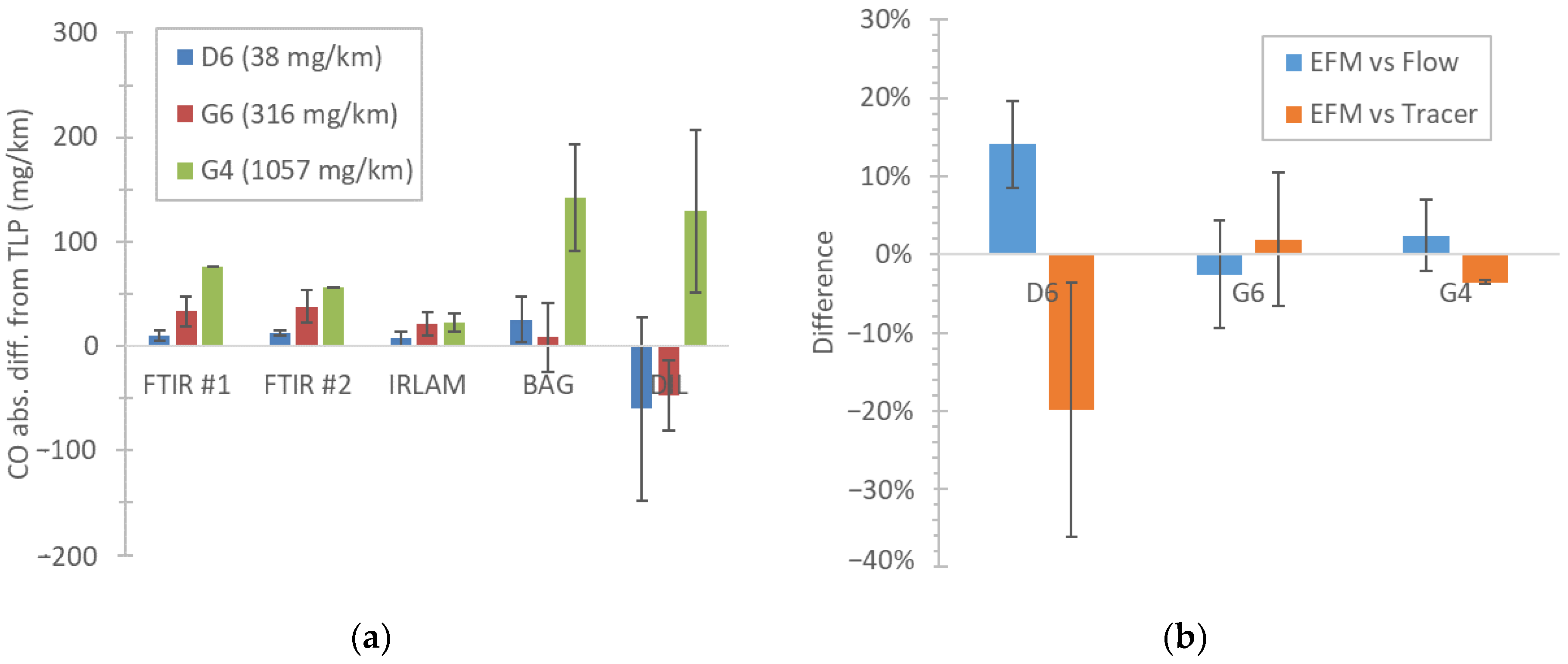
3. Results
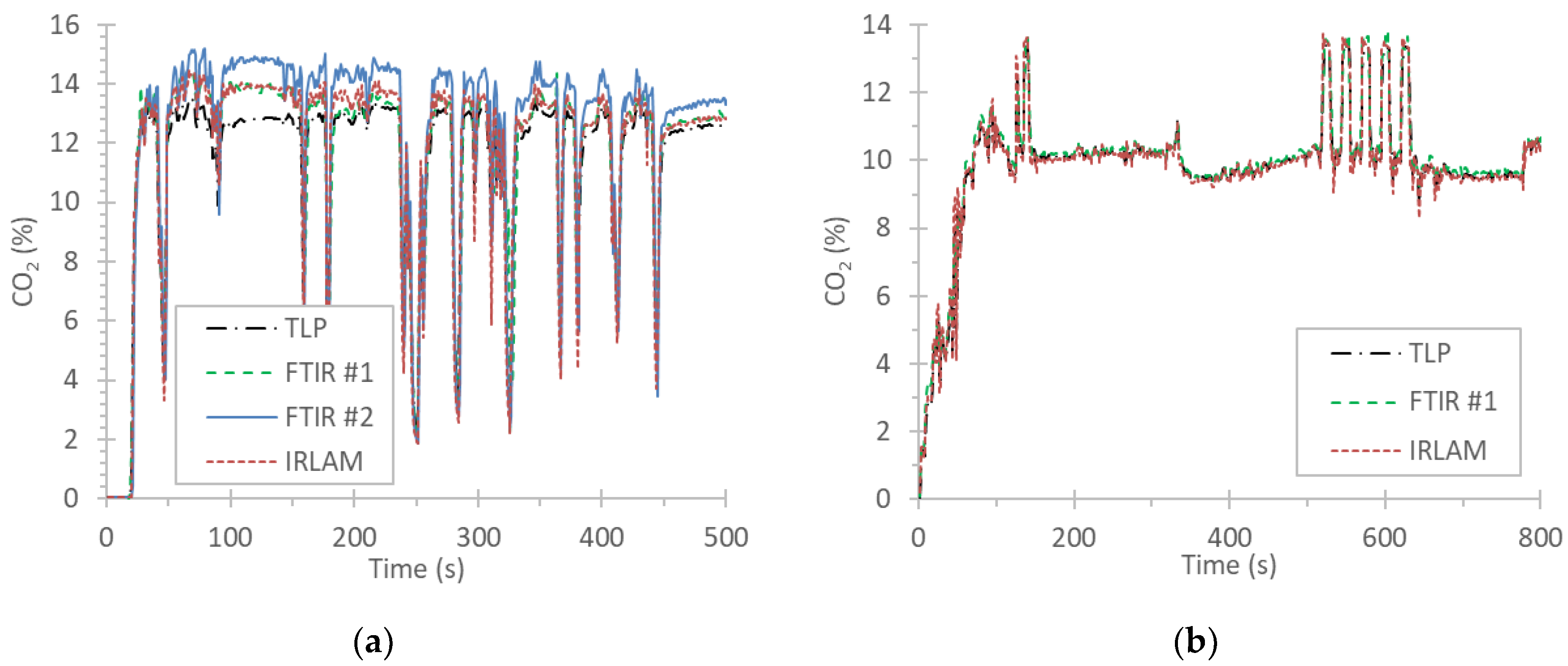
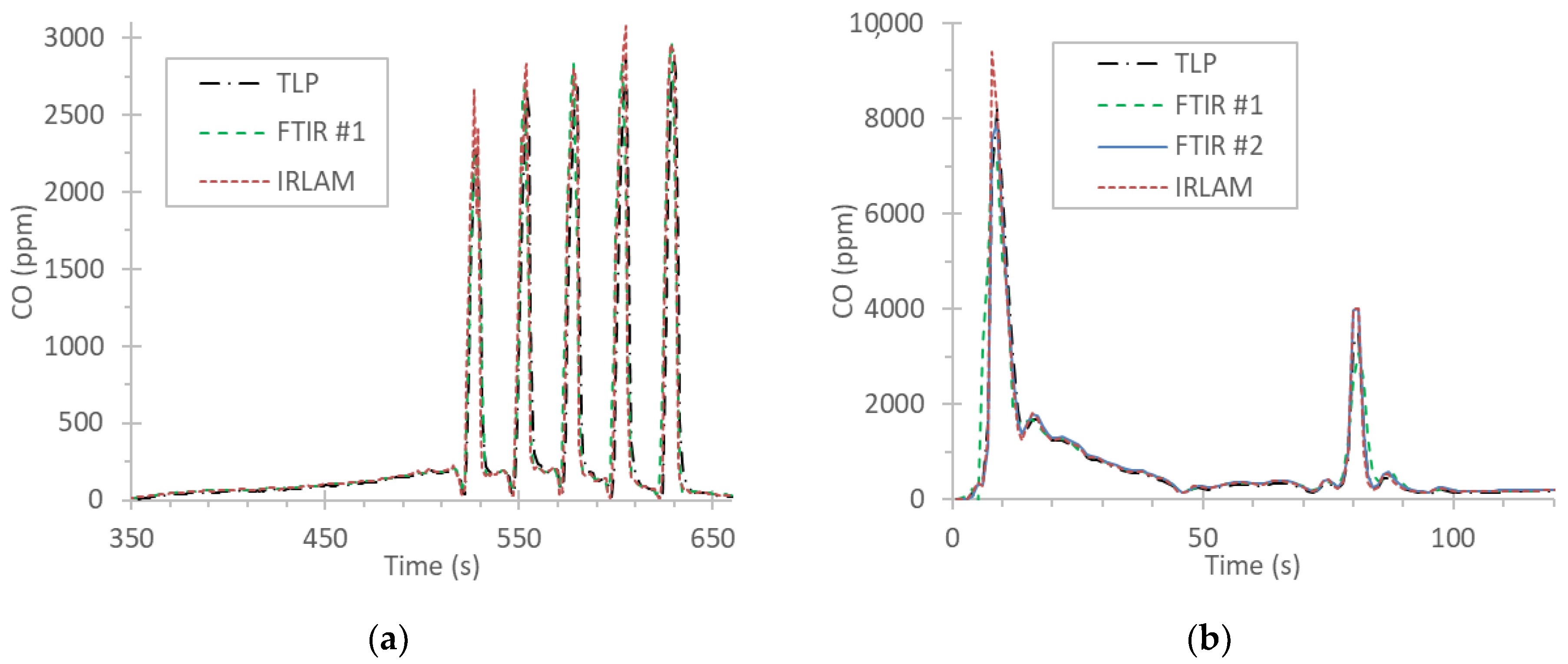
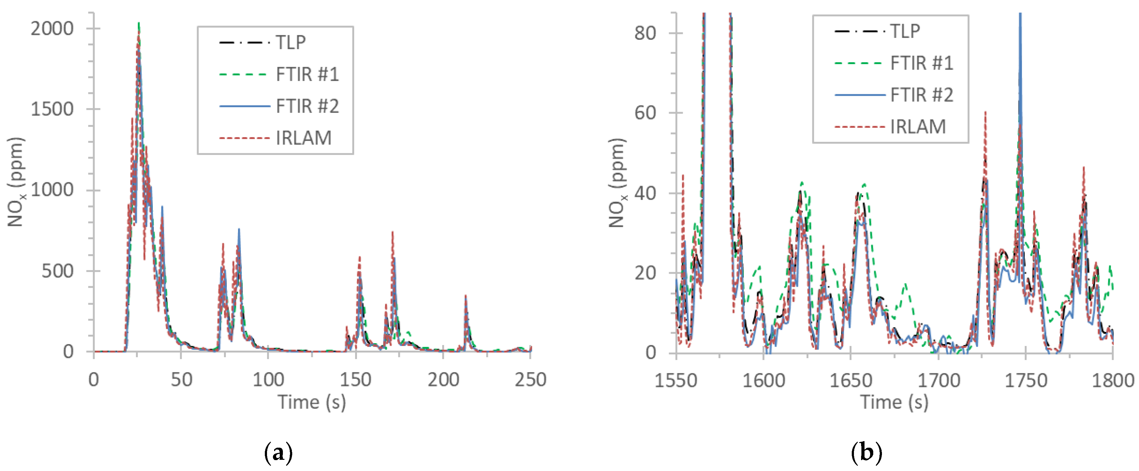
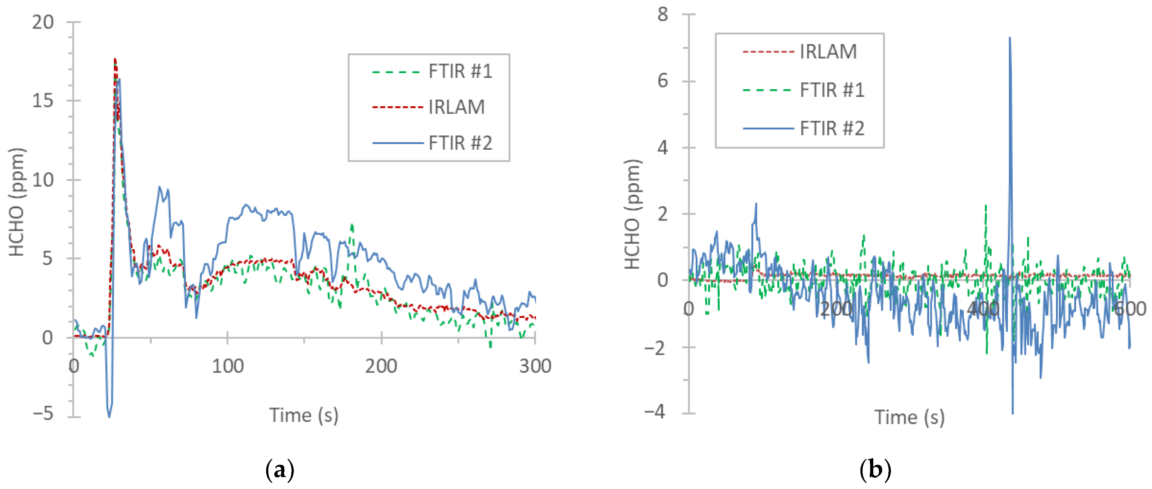
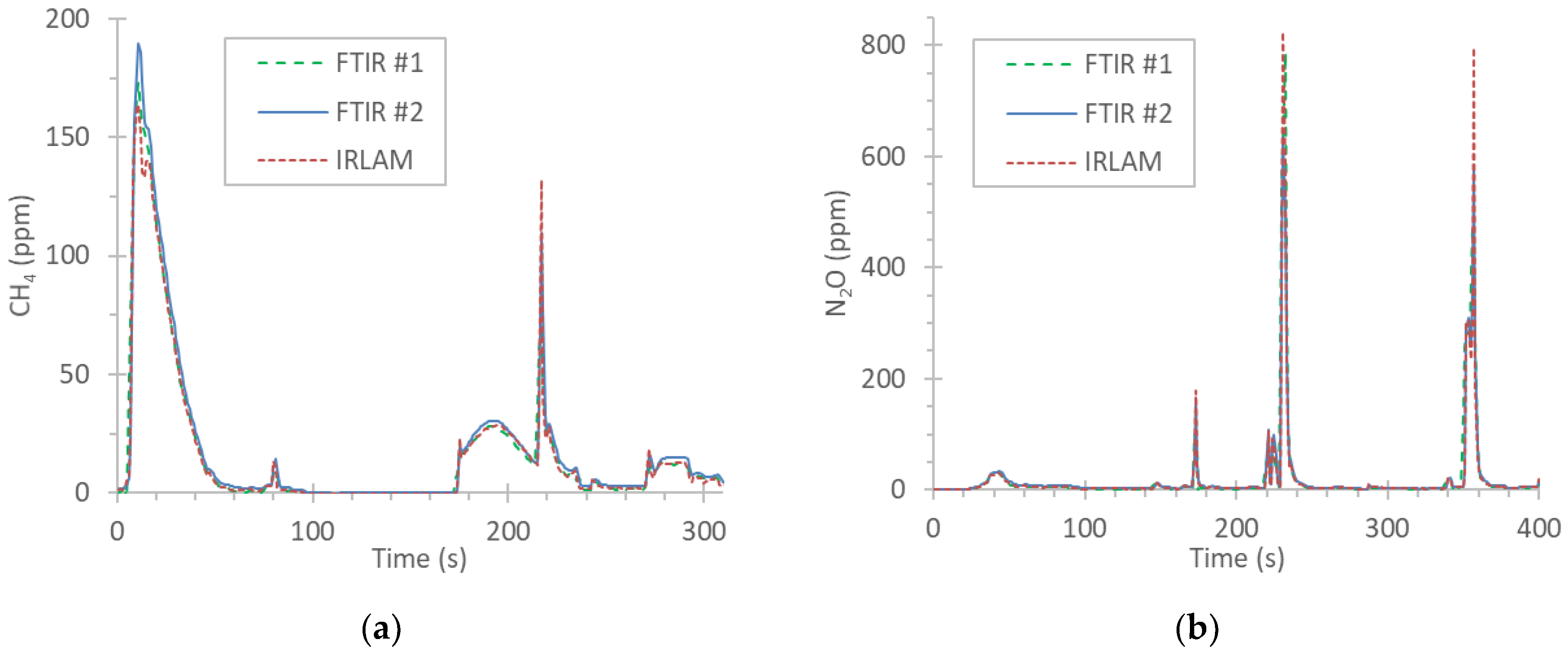
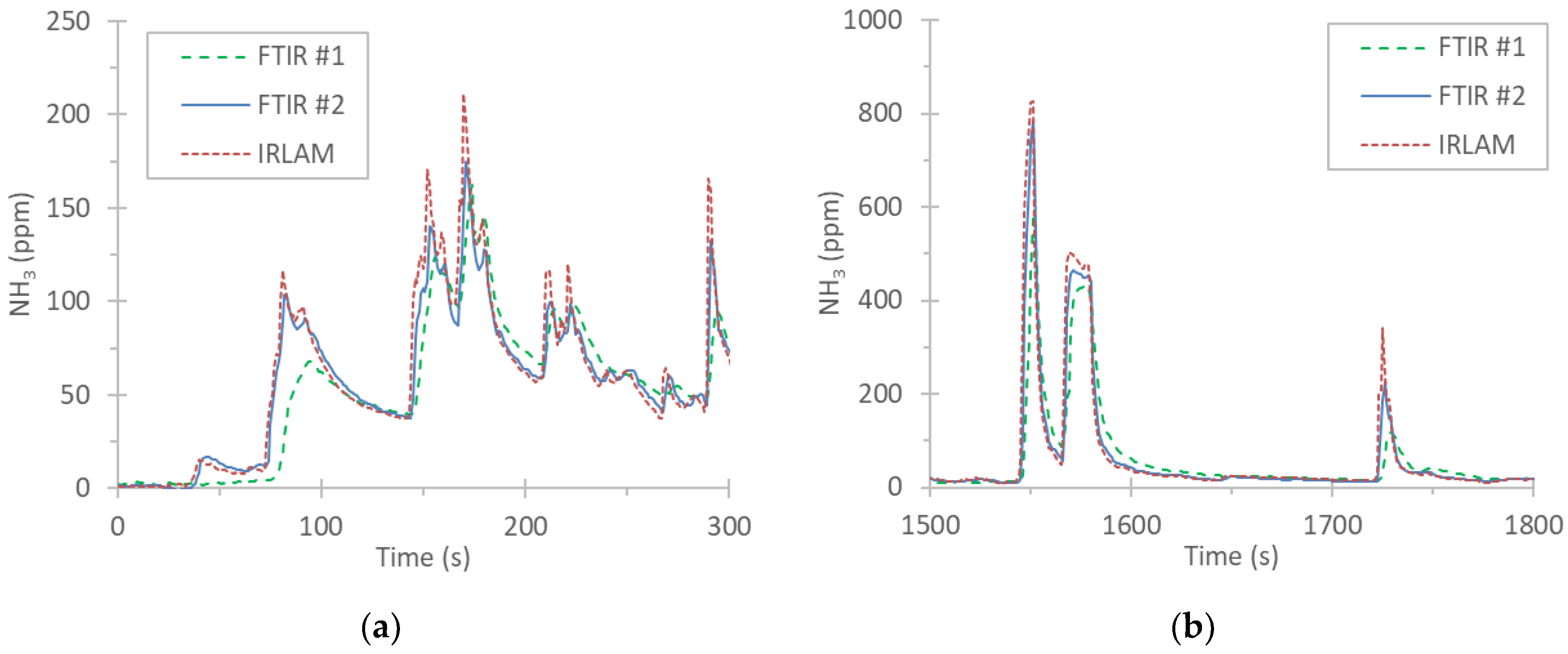
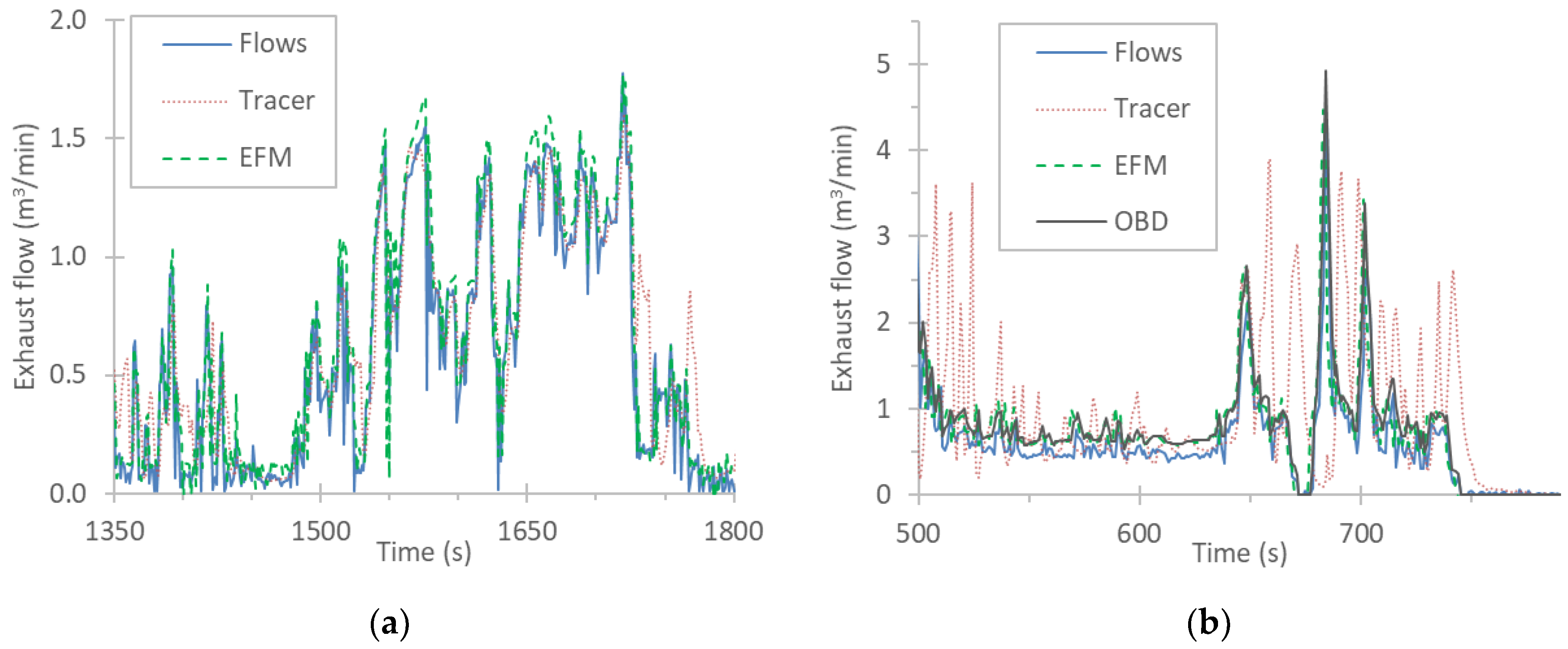
3.1. Real Time Examples
3.2. Integrated Results
4. Discussion
5. Conclusions
Author Contributions
Funding
Data Availability Statement
Acknowledgments
Conflicts of Interest
Abbreviations
| BAB | Bundesautobahn (federal highway); |
| BAG | bags |
| C | concentration |
| CH4 | methane |
| CLD | chemiluminescence detection |
| CNG | compressed natural gas |
| CO | carbon monoxide |
| CO2 | carbon dioxide |
| CVS | constant volume sampling |
| DA | dilution air |
| DIL | diluted |
| DOC | Diesel oxidation catalyst |
| DPF | Diesel particulate filter |
| EFM | exhaust flow meter |
| EGR | exhaust-gas recirculation |
| EU | European Union |
| FCM | fuel consumption monitoring |
| FID | flame ionization detection |
| FTIR | Fourier-transform infrared |
| GC | gas chromatography |
| GPF | gasoline particulate filter |
| GWP | global warming potential |
| HCHO | formaldehyde |
| HD | heavy-duty |
| IARC | International Agency for Research on Cancer |
| ICE | internal combustion engine |
| IPCC | Intergovernmental Panel on Climate Change |
| IRLAM | infrared laser absorption modulation |
| ISC | in-service conformity |
| JRC | Joint Research Center |
| LD | light-duty |
| LNT | lean NOx trap |
| m | mass rate |
| N2O | nitrous oxide |
| NDIR | non-dispersive infrared |
| NH3 | ammonia |
| NMHC | non-methane hydrocarbons |
| NMOG | non-methane organic gases |
| NO2 | nitrogen dioxide |
| NOx | nitrogen oxides |
| OBD | on-board diagnostics |
| PEMS | portable emissions measurement system |
| PM | particulate matter |
| Q | flow rate |
| QCL-IR | quantum cascade laser infrared |
| RDE | real-driving emissions |
| RDE_D | real-driving emissions dynamic |
| RDE_S | real-driving emissions short |
| SAO | smooth-approach orifice |
| SCR | selective-catalytic reduction |
| TfL | Transport for London |
| THC | total hydrocarbons |
| TLP | tailpipe |
| TWC | three-way catalyst |
| VELA | vehicle emissions laboratory |
| WHO | World Health Organization |
| WLTC | worldwide harmonized light-vehicles test cycle |
Appendix A

| Analyzer | BAG | DIL | TLP | FTIR #1 | FTIR #2 | IRLAM |
|---|---|---|---|---|---|---|
| Manufacturer | HORIBA | HORIBA | HORIBA | AVL | HORIBA | HORIBA |
| Model | MEXA-7400 | MEXA-7400 | MEXA-7100 | Sesam i60 | FTX-ONE | IRLAM PEMS |
| CO2 | 1%/5% | 3% | 20% | 1%/20% | 1%/5%/20% | 20% |
| CO | 10/200/500 | 1000 | 12% | 50/8000/10% | 200/5000/10% | 1%/12% |
| NO | - | - | - | 50/1000/1% | 200/1000/5000 | 2000 |
| NO2 | - | - | - | 25/1000 | 200 | 800 |
| NOx | 20/50 | 500 | 500/1% | - | - | - |
| N2O | - | - | - | 25/1000 | 200 | 1000 |
| NH3 | - | - | - | 50/1000 | 100/1000 | 1500 |
| HCHO | - | - | - | 20/1000 | 500 | 500 |
| CH4 | 5/10 | - | - | 50/1000 | 500/1% | 2000/1% |
Appendix B
| Analyzer | BAG | DIL 1 | TLP 1 | FTIR #1 2 | FTIR #2 3 | IRLAM 4 |
|---|---|---|---|---|---|---|
| Manufacturer | HORIBA | HORIBA | HORIBA | AVL | HORIBA | HORIBA |
| Model | MEXA-7400 | MEXA-7400 | MEXA-7100 | Sesam i60 | FTX-ONE | IRLAM PEMS |
| CO2 | n.a. | 2.40 | 2.60 | 130 | 0.64 | 39.00 |
| CO | n.a. | 0.04 | 2.70 | 1.2 | 0.09 | 0.84 |
| NO | - | - | - | 1.0 | 0.35 | 0.19 |
| NO2 | - | - | - | 0.4 | 0.05 | 0.09 |
| NOx | n.a. | 0.03 | 0.03 | - | - | - |
| N2O | - | - | - | 0.4 | 0.06 | 0.07 |
| NH3 | - | - | - | 0.5 | 0.05 | 0.07 |
| HCHO | - | - | - | 0.6 | 0.20 | 0.04 |
| CH4 | n.a. | - | - | 0.5 | 0.06 | 0.16 |

References
- European Environmental Agency (EEA). Air Quality in Europe 2022. Report No. 05/2022; ISBN 978-92-9480-515-7. Available online: https://www.eea.europa.eu/publications/air-quality-in-europe-2022 (accessed on 30 January 2023).
- Eurostat Mortality and Life Expectancy Statistics. Available online: https://ec.europa.eu/eurostat/statistics-explained/index.php?title=mortality_and_life_expectancy_statistics2022 (accessed on 30 January 2023).
- DieselNet Emission Standards. Available online: https://dieselnet.com/standards/ (accessed on 30 January 2023).
- Giechaskiel, B.; Melas, A.; Martini, G.; Dilara, P. Overview of Vehicle Exhaust Particle Number Regulations. Processes 2021, 9, 2216. [Google Scholar] [CrossRef]
- European Environmental Agency (EEA). Air Pollutant Emissions Data Viewer (Gothenburg Protocol, LRTAP Convention) 1990–2020. Available online: https://www.eea.europa.eu/data-and-maps/dashboards/air-pollutant-emissions-data-viewer-42021 (accessed on 30 January 2023).
- European Commission. Joint Research Centre. On-Road Testing with Portable Emissions Measurement Systems (PEMS): Guidance Note for Light Duty Vehicles; Publications Office: Luxembourg, 2018. [Google Scholar]
- European Commission. Joint Research Centre. Institute for Energy and Transport. PEMS Based In-Service Testing: Practical Recommendations for Heavy Duty Engines/Vehicles; Publications Office: Luxembourg, 2015. [Google Scholar]
- Giechaskiel, B.; Clairotte, M.; Valverde-Morales, V.; Bonnel, P.; Kregar, Z.; Franco, V.; Dilara, P. Framework for the Assessment of PEMS (Portable Emissions Measurement Systems) Uncertainty. Environ. Res. 2018, 166, 251–260. [Google Scholar] [CrossRef]
- Leso, V.; Macrini, M.C.; Russo, F.; Iavicoli, I. Formaldehyde Exposure and Epigenetic Effects: A Systematic Review. Appl. Sci. 2020, 10, 2319. [Google Scholar] [CrossRef]
- Wang, M.; Hu, K.; Chen, W.; Shen, X.; Li, W.; Lu, X. Ambient Non-Methane Hydrocarbons (NMHCs) Measurements in Baoding, China: Sources and Roles in Ozone Formation. Atmosphere 2020, 11, 1205. [Google Scholar] [CrossRef]
- Zhu, L.; Henze, D.K.; Bash, J.O.; Cady-Pereira, K.E.; Shephard, M.W.; Luo, M.; Capps, S.L. Sources and Impacts of Atmospheric NH3: Current Understanding and Frontiers for Modeling, Measurements, and Remote Sensing in North America. Curr. Pollut. Rep. 2015, 1, 95–116. [Google Scholar] [CrossRef]
- European Commission Euro 7 Proposal. Available online: https://single-market-economy.ec.europa.eu/sectors/automotive-industry/environmental-protection/emissions-automotive-sector_en2022 (accessed on 30 January 2023).
- Selleri, T.; Melas, A.D.; Joshi, A.; Manara, D.; Perujo, A.; Suarez-Bertoa, R. An Overview of Lean Exhaust DeNOx Aftertreatment Technologies and NOx Emission Regulations in the European Union. Catalysts 2021, 11, 404. [Google Scholar] [CrossRef]
- Martinovic, F.; Castoldi, L.; Deorsola, F.A. Aftertreatment Technologies for Diesel Engines: An Overview of the Combined Systems. Catalysts 2021, 11, 653. [Google Scholar] [CrossRef]
- Castoldi, L. An Overview on the Catalytic Materials Proposed for the Simultaneous Removal of NOx and Soot. Materials 2020, 13, 3551. [Google Scholar] [CrossRef]
- Rood, S.; Eslava, S.; Manigrasso, A.; Bannister, C. Recent Advances in Gasoline Three-Way Catalyst Formulation: A Review. Proceedings of the Institution of Mechanical Engineers, Part D. J. Automob. Eng. 2020, 234, 936–949. [Google Scholar] [CrossRef]
- Selleri, T.; Gioria, R.; Melas, A.D.; Giechaskiel, B.; Forloni, F.; Mendoza Villafuerte, P.; Demuynck, J.; Bosteels, D.; Wilkes, T.; Simons, O.; et al. Measuring Emissions from a Demonstrator Heavy-Duty Diesel Vehicle under Real-World Conditions—Moving Forward to Euro VII. Catalysts 2022, 12, 184. [Google Scholar] [CrossRef]
- Suarez-Bertoa, R.; Gioria, R.; Selleri, T.; Lilova, V.; Melas, A.; Onishi, Y.; Franzetti, J.; Forloni, F.; Perujo, A. NH3 and N2O Real World Emissions Measurement from a CNG Heavy Duty Vehicle Using On-Board Measurement Systems. Appl. Sci. 2021, 11, 10055. [Google Scholar] [CrossRef]
- Suarez-Bertoa, R.; Selleri, T.; Gioria, R.; Melas, A.D.; Ferrarese, C.; Franzetti, J.; Arlitt, B.; Nagura, N.; Hanada, T.; Giechaskiel, B. Real-Time Measurements of Formaldehyde Emissions from Modern Vehicles. Energies 2022, 15, 7680. [Google Scholar] [CrossRef]
- Giechaskiel, B.; Clairotte, M. Fourier Transform Infrared (FTIR) Spectroscopy for Measurements of Vehicle Exhaust Emissions: A Review. Appl. Sci. 2021, 11, 7416. [Google Scholar] [CrossRef]
- Onishi, Y.; Hamauchi, S.; Shibuya, K.; McWilliams-Ward, K.; Akita, M.; Tsurumi, K. Development of On-Board NH3 and N2O Analyzer Utilizing Mid-Infrared Laser Absorption Spectroscopy; SAE Technical Paper 2021-01-0610; SAE: Warrendale, PA, USA, 2021. [Google Scholar] [CrossRef]
- Hara, K.; Shibuya, K.; Nagura, N.; Hanada, T.; Tsurumi, K. Formaldehydes Measurement Using Laser Spectroscopic Gas Analyzer; SAE Technical Paper 2021-01-0604; SAE: Warrendale, PA, USA, 2021. [Google Scholar] [CrossRef]
- Shibuya, K.; Podzorov, A.; Matsuhama, M.; Nishimura, K.; Magari, M. High-Sensitivity and Low-Interference Gas Analyzer with Feature Extraction from Mid-Infrared Laser Absorption-Modulated Signal. Meas. Sci. Technol. 2021, 32, 035201. [Google Scholar] [CrossRef]
- Lamas, J.E.; Hara, K.; Mori, Y. Optimization of Automotive Exhaust Sampling Parameters for Evaluation of After-Treatment Systems Using FTIR Exhaust Gas Analyzers; SAE Technical Paper 2019-01-0746; SAE: Warrendale, PA, USA, 2019. [Google Scholar] [CrossRef]
- Sherman, M.T.; Chase, R.; Mauti, A.; Rauker, Z.; Silvis, W. Evaluation of Horiba MEXA 7000 Bag Bench Analyzers for Single Range Operation. SAE Trans. 1999, 108, 90–111. [Google Scholar]
- Giechaskiel, B.; Zardini, A.A.; Clairotte, M. Exhaust Gas Condensation during Engine Cold Start and Application of the Dry-Wet Correction Factor. Appl. Sci. 2019, 9, 2263. [Google Scholar] [CrossRef]
- Giechaskiel, B.; Zardini, A.A.; Lahde, T.; Clairotte, M.; Forloni, F.; Drossinos, Y. Identification and Quantification of Uncertainty Components in Gaseous and Particle Emission Measurements of a Moped. Energies 2019, 12, 4343. [Google Scholar] [CrossRef]
- Giechaskiel, B.; Valverde, V.; Kontses, A.; Melas, A.; Martini, G.; Balazs, A.; Andersson, J.; Samaras, Z.; Dilara, P. Particle Number Emissions of a Euro 6d-Temp Gasoline Vehicle under Extreme Temperatures and Driving Conditions. Catalysts 2021, 11, 607. [Google Scholar] [CrossRef]
- Kelly, N.A.; Groblicki, P.J. Real-World Emissions from a Modern Production Vehicle Driven in Los Angeles. Air Waste 1993, 43, 1351–1357. [Google Scholar] [CrossRef]
- Jetter, J.; Maeshiro, S.; Hatcho, S.; Klebba, R. Development of an On-Board Analyzer for Use on Advanced Low Emission Vehicles. SAE Trans. 2000, 109, 755–762. [Google Scholar]
- Giechaskiel, B.; Bonnel, P.; Perujo, A.; Dilara, P. Solid Particle Number (SPN) Portable Emissions Measurement Systems (PEMS) in the European Legislation: A Review. Int. J. Environ. Res. Public Health 2019, 16, 4819. [Google Scholar] [CrossRef] [PubMed]
- Weiss, M.; Bonnel, P.; Kühlwein, J.; Provenza, A.; Lambrecht, U.; Alessandrini, S.; Carriero, M.; Colombo, R.; Forni, F.; Lanappe, G.; et al. Will Euro 6 Reduce the NOx Emissions of New Diesel Cars?—Insights from on-Road Tests with Portable Emissions Measurement Systems (PEMS). Atmos. Environ. 2012, 62, 657–665. [Google Scholar] [CrossRef]
- Buckingham, J.P.; Mason, R.L.; Spears, M.W. Determination of PEMS Measurement Allowances for Gaseous Emissions Regulated Under the Heavy-Duty Diesel Engine In-Use Testing Program Part 2—Statistical Modeling and Simulation Approach. SAE Int. J. Fuels Lubr. 2009, 2, 422–434. [Google Scholar] [CrossRef]
- Cao, T.; Durbin, T.D.; Cocker, D.R.; Wanker, R.; Schimpl, T.; Pointner, V.; Oberguggenberger, K.; Johnson, K.C. A Comprehensive Evaluation of a Gaseous Portable Emissions Measurement System with a Mobile Reference Laboratory. Emiss. Control. Sci. Technol. 2016, 2, 173–180. [Google Scholar] [CrossRef]
- Giechaskiel, B.; Jakobsson, T.; Karlsson, H.L.; Khan, M.Y.; Kronlund, L.; Otsuki, Y.; Bredenbeck, J.; Handler-Matejka, S. Assessment of On-Board and Laboratory Gas Measurement Systems for Future Heavy-Duty Emissions Regulations. Int. J. Environ. Res. Public Health 2022, 19, 6199. [Google Scholar] [CrossRef] [PubMed]
- Daham, B.; Andrews, G.E.; Li, H.; Ballesteros, R.; Bell, M.C.; Tate, J.; Ropkins, K. Application of a Portable FTIR for Measuring On-Road Emissions; SAE Technical Paper 2005-01-0676; SAE: Warrendale, PA, USA, 2005. [Google Scholar] [CrossRef]
- Li, H.; Ropkins, K.; Andrews, G.E.; Daham, B.; Bell, M.; Tate, J.; Hawley, G. Evaluation of a FTIR Emission Measurement System for Legislated Emissions Using a SI Car; SAE Technical Paper; SAE: Warrendale, PA, USA, 2006; ISBN 0-7680-1803-X. [Google Scholar]
- Wallner, T.; Frazee, R. Study of Regulated and Non-Regulated Emissions from Combustion of Gasoline, Alcohol Fuels and Their Blends in a DI-SI Engine; SAE Technical Paper 2010-01-1571; SAE: Warrendale, PA, USA, 2010. [Google Scholar] [CrossRef]
- Czerwinski, J.; Comte, P.; Güdel, M.; Mayer, A.; Lemaire, J.; Reutimann, F.; Berger, A.H. Investigations of NO2 in Legal Test Procedure for Diesel Passenger Cars; SAE Technical Paper 2015-24-2510; SAE: Warrendale, PA, USA, 2015. [Google Scholar] [CrossRef]
- Zhang, F.; Wang, J.; Tian, D.; Wang, J.-X.; Shuai, S.-J. Research on Unregulated Emissions from an Alcohols-Gasoline Blend Vehicle Using FTIR, HPLC and GC-MS Measuring Methods. SAE Int. J. Engines 2013, 6, 1126–1137. [Google Scholar] [CrossRef]
- Olsen, D.B.; Kohls, M.; Arney, G. Impact of Oxidation Catalysts on Exhaust NO2/NOx Ratio from Lean-Burn Natural Gas Engines. J. Air Waste Manag. Assoc. 2010, 60, 867–874. [Google Scholar] [CrossRef]
- Vojtíšek-Lom, M.; Beránek, V.; Klír, V.; Jindra, P.; Pechout, M.; Voříšek, T. On-Road and Laboratory Emissions of NO, NO2, NH3, N2O and CH4 from Late-Model EU Light Utility Vehicles: Comparison of Diesel and CNG. Sci. Total Environ. 2018, 616–617, 774–784. [Google Scholar] [CrossRef]
- Suarez-Bertoa, R.; Pechout, M.; Vojtíšek, M.; Astorga, C. Regulated and Non-Regulated Emissions from Euro 6 Diesel, Gasoline and CNG Vehicles under Real-World Driving Conditions. Atmosphere 2020, 11, 204. [Google Scholar] [CrossRef]
- Varella, R.; Giechaskiel, B.; Sousa, L.; Duarte, G. Comparison of Portable Emissions Measurement Systems (PEMS) with Laboratory Grade Equipment. Appl. Sci. 2018, 8, 1633. [Google Scholar] [CrossRef]
- Giechaskiel, B.; Casadei, S.; Mazzini, M.; Sammarco, M.; Montabone, G.; Tonelli, R.; Deana, M.; Costi, G.; Di Tanno, F.; Prati, M.; et al. Inter-Laboratory Correlation Exercise with Portable Emissions Measurement Systems (PEMS) on Chassis Dynamometers. Appl. Sci. 2018, 8, 2275. [Google Scholar] [CrossRef]
- Giechaskiel, B.; Casadei, S.; Rossi, T.; Forloni, F.; Di Domenico, A. Measurements of the Emissions of a “Golden” Vehicle at Seven Laboratories with Portable Emission Measurement Systems (PEMS). Sustainability 2021, 13, 8762. [Google Scholar] [CrossRef]
- Valverde, V.; Giechaskiel, B. Assessment of Gaseous and Particulate Emissions of a Euro 6d-Temp Diesel Vehicle Driven >1300 km Including Six Diesel Particulate Filter Regenerations. Atmosphere 2020, 11, 645. [Google Scholar] [CrossRef]
- Collins, J.F.; Shepherd, P.; Durbin, T.D.; Lents, J.; Norbeck, J.; Barth, M. Measurements of In-Use Emissions from Modern Vehicles Using an on-Board Measurement System. Environ. Sci. Technol. 2007, 41, 6554–6561. [Google Scholar] [CrossRef] [PubMed]
- Seykens, X.; van den Tillaart, E.; Lilova, V.; Nakatani, S. NH3 Measurements for Advanced SCR Applications; SAE Technical Paper 2016-01-0975; SAE: Warrendale, PA, USA.
- Suarez-Bertoa, R.; Mendoza-Villafuerte, P.; Riccobono, F.; Vojtisek, M.; Pechout, M.; Perujo, A.; Astorga, C. On-Road Measurement of NH3 Emissions from Gasoline and Diesel Passenger Cars during Real World Driving Conditions. Atmos. Environ. 2017, 166, 488–497. [Google Scholar] [CrossRef]
- Rahman, M.; Hara, K.; Nakatani, S.; Tanaka, Y. Development of a Fast Response Nitrogen Compounds Analyzer Using Quantum Cascade Laser for Wide-Range Measurement; SAE Technical Paper 2011-26-0044; SAE: Warrendale, PA, USA, 2011. [Google Scholar] [CrossRef]
- Suarez-Bertoa, R.; Zardini, A.A.; Lilova, V.; Meyer, D.; Nakatani, S.; Hibel, F.; Ewers, J.; Clairotte, M.; Hill, L.; Astorga, C. Intercomparison of Real-Time Tailpipe Ammonia Measurements from Vehicles Tested over the New World-Harmonized Light-Duty Vehicle Test Cycle (WLTC). Env. Sci. Pollut. Res. 2015, 22, 7450–7460. [Google Scholar] [CrossRef]
- Li, N.; El-Hamalawi, A.; Barrett, R.; Baxter, J. Ammonia Measurement Investigation Using Quantum Cascade Laser and Two Different Fourier Transform Infrared Spectroscopy Methods; SAE Technical Paper 2020-01-0365; SAE: Warrendale, PA, USA, 2020. [Google Scholar] [CrossRef]
- Murtonen, T.; Vesala, H.; Koponen, P.; Pettinen, R.; Kajolinna, T.; Antson, O. NH3 Sensor Measurements in Different Engine Applications; SAE Technical Paper 2018-01-1814; SAE: Warrendale, PA, USA, 2018. [Google Scholar] [CrossRef]
- Wright, N.; Osborne, D.; Music, N. Comparison of Hydrocarbon Measurement with FTIR and FID in a Dual Fuel Locomotive Engine; SAE Technical Paper 2016-01-0978; SAE: Warrendale, PA, USA, 2016. [Google Scholar] [CrossRef]
- Suarez-Bertoa, R.; Clairotte, M.; Arlitt, B.; Nakatani, S.; Hill, L.; Winkler, K.; Kaarsberg, C.; Knauf, T.; Zijlmans, R.; Boertien, H.; et al. Intercomparison of Ethanol, Formaldehyde and Acetaldehyde Measurements from a Flex-Fuel Vehicle Exhaust during the WLTC. Fuel 2017, 203, 330–340. [Google Scholar] [CrossRef]
- Daemme, L.C.; Penteado, R.; Corrêa, S.M.; Zotin, F.; Errera, M.R. Emissions of Criteria and Non-Criteria Pollutants by a Flex-Fuel Motorcycle. J. Braz. Chem. Soc. 2016, 27, 2192–2202. [Google Scholar] [CrossRef]


| Analyzer | BAG | DIL | TLP | FTIR #1 | FTIR #2 | IRLAM |
|---|---|---|---|---|---|---|
| Manufacturer | HORIBA | HORIBA | HORIBA | AVL | HORIBA | HORIBA |
| Model | MEXA-7400 | MEXA-7400 | MEXA-7100 | Sesam i60 | FTX-ONE | IRLAM PEMS |
| CO2 | NDIR | NDIR | NDIR | FTIR | FTIR | QCL-IR |
| CO | NDIR | NDIR | NDIR | FTIR | FTIR | QCL-IR |
| NOx (NO + NO2) | CLD | CLD | CLD | FTIR | FTIR | QCL-IR |
| N2O | - | - | - | FTIR | FTIR | QCL-IR |
| NH3 | - | - | - | FTIR | FTIR | QCL-IR |
| HCHO | - | - | - | FTIR | FTIR | QCL-IR |
| CH4 | GC-FID | - | - | FTIR | FTIR | QCL-IR |
| Sampling line T (°C) | - | 191 | 191 | 191 | 191 | 113 |
| Analyser t10-90 (s) | - | 2.5 | 2.5 | 2.0 | 1.5 1 | 1.0 2 |
| Qs (L/min) | - | 11 | 11 | 6.5 | 3.5 | 3.3 |
| Characteristics | D6 | G6 | G4 |
|---|---|---|---|
| Vehicle category | M1 | M1 | M1 |
| Cylinders/arrangement | 4-inline | 4-inline | 4-inline |
| Combustion type | Compression ignition | Positive ignition | Positive ignition |
| Fuel type | Diesel | Gasoline | Gasoline |
| Injection type | Direct | Port-fuel | Port-fuel |
| Aspiration type | Turbocharged | Turbocharged | Natural aspiration |
| Engine displacement (cm3) | 1998 | 1598 | 1108 |
| ICE engine power (kW) | 150 | 69 | 40 |
| Electric engine V/power (kW) | 48 V/13.3 kW | 245 V/51 kW | - |
| Emission control technology | DOC, DPF, EGR, SCR, LNT | TWC, GPF | TWC |
| Transmission/gearbox | Automatic | Automatic | Manual |
| Test mass (kg) | 1903 | 1635 | 1020 |
| Registration date | July 2021 | September 2022 | August 2006 |
| Mileage (km) | 21,000 | 9000 | 25,700 |
| Emission standard | Euro 6d-ISC-FCM | Euro 6d-ISC-FCM | Euro 4 |
| Cycle | WLTC | BAB | TfL | RDE_S | RDE_D |
|---|---|---|---|---|---|
| Distance (km) | 23.2 | 24.9 | 8.8 | 28.3 | 91.7 |
| Duration (s) | 1800 | 800 | 2320 | 1830 | 5400 |
| Mean speed (km/h) | 46.2 | 111.5 | 13.7 | 54.9 | 61.0 |
| Max speed (km/h) | 131.3 | 131.1 | 51.8 | 130.7 | 143.6 |
| Component | Proposed Limit (Euro 7) | Examined Range (All Vehicles) | Uncertainty 1 |
|---|---|---|---|
| CO2 | – | 90–210 g/km | 10–15 g/km |
| CO | 500 mg/km | 5–1085 mg/km | 50 mg/km or 15% 2 |
| NOx | 60 mg/km | 1–72 mg/km | 10–15 mg/km |
| CH4 3 | (32 mg/km)– | 1–20 mg/km | 1–2 mg/km |
| HCHO | – | 0–1.7 mg/km | 1 mg/km |
| NH3 | 20 mg/km | 1–23 mg/km | 1.5–3.5 mg/km |
| N2O | – | 0–42 mg/km | 1 mg/km |
| Exhaust flow 4 | – | 0.1–2.3 m3/min | 10–20% |
Disclaimer/Publisher’s Note: The statements, opinions and data contained in all publications are solely those of the individual author(s) and contributor(s) and not of MDPI and/or the editor(s). MDPI and/or the editor(s) disclaim responsibility for any injury to people or property resulting from any ideas, methods, instructions or products referred to in the content. |
© 2023 by the authors. Licensee MDPI, Basel, Switzerland. This article is an open access article distributed under the terms and conditions of the Creative Commons Attribution (CC BY) license (https://creativecommons.org/licenses/by/4.0/).
Share and Cite
Valverde, V.; Kondo, Y.; Otsuki, Y.; Krenz, T.; Melas, A.; Suarez-Bertoa, R.; Giechaskiel, B. Measurement of Gaseous Exhaust Emissions of Light-Duty Vehicles in Preparation for Euro 7: A Comparison of Portable and Laboratory Instrumentation. Energies 2023, 16, 2561. https://doi.org/10.3390/en16062561
Valverde V, Kondo Y, Otsuki Y, Krenz T, Melas A, Suarez-Bertoa R, Giechaskiel B. Measurement of Gaseous Exhaust Emissions of Light-Duty Vehicles in Preparation for Euro 7: A Comparison of Portable and Laboratory Instrumentation. Energies. 2023; 16(6):2561. https://doi.org/10.3390/en16062561
Chicago/Turabian StyleValverde, Victor, Yosuke Kondo, Yoshinori Otsuki, Torsten Krenz, Anastasios Melas, Ricardo Suarez-Bertoa, and Barouch Giechaskiel. 2023. "Measurement of Gaseous Exhaust Emissions of Light-Duty Vehicles in Preparation for Euro 7: A Comparison of Portable and Laboratory Instrumentation" Energies 16, no. 6: 2561. https://doi.org/10.3390/en16062561
APA StyleValverde, V., Kondo, Y., Otsuki, Y., Krenz, T., Melas, A., Suarez-Bertoa, R., & Giechaskiel, B. (2023). Measurement of Gaseous Exhaust Emissions of Light-Duty Vehicles in Preparation for Euro 7: A Comparison of Portable and Laboratory Instrumentation. Energies, 16(6), 2561. https://doi.org/10.3390/en16062561