Article

Numerical Assessment of a Two-Phase Model for Propulsive Pump Performance Prediction

Department of Industrial Engineering, Università degli Studi di Padova, 35131 Padova, Italy
*
Author to whom correspondence should be addressed.
Energies 2023, 16(18), 6592; https://doi.org/10.3390/en16186592
Submission received: 16 August 2023 / Revised: 9 September 2023 / Accepted: 11 September 2023 / Published: 13 September 2023
(This article belongs to the Special Issue Advanced Applications of Solar and Thermal Storage Energy)

Abstract

:
The present work provides a detailed numerical investigation of a turbopump for waterjet applications in cavitating conditions. In particular, the study focuses on the complexities of cavitation modelling, serving as a pivotal reference for future computational research, especially in off-design hydro-jet scenarios, and it aims to extend current model assessments of the existing methods, by disputing their standard formulations. Thus, a computational domain of a single rotor-stator blade passage is solved using steady-state Reynolds-Averaged Navier–Stokes equations, coupled with one-, two-, and four-equation turbulence models, and compared with available measurements, encompassing both nominal and thrust breakdown conditions. Through grid dependency analysis, a medium refinement with the Shear Stress Transport turbulence model is chosen as the optimal configuration, reducing either computational time and relative error in breakdown efficiency to 1%. This arrangement is coupled with a systematic study of the Zwart cavitation model parameters through multipliers ranging from 10 2 to 10 2 . Results reveal that properly tuning these values allows for a more accurate reconstruction of the initial phases of cavitation up to breakdown. Notably, increasing the nucleation radius reduces the difference between the estimated head rise and experimental values near breakdown, reducing the maximum error by 4%. This variation constrains vapour concentration, promoting cavitation volume extension in the passage. A similar observation occurs when modifying the condensation coefficient, whereas altering the vaporization coefficient yields opposite effects.

1. Introduction

Nowadays, both in military and civilian applications, high-speed vessels widely benefit from efficient propulsion generated through axial-flow pump-driven waterjets. Thus, the associated turbomachinery represents a fundamental driver for the design of these devices [1,2]. Bladed components are responsible for converting the shaft energy provided by the engines into a pressure rise of the fluid to be exploited for the momentum imbalance as it accelerates through the nozzle [3]. With the increasing demand for faster transport, a well-known operating limitation of these machines is the occurrence of cavitation [4]. This phenomenon involves the formation of vapour bubbles, or cavities, in field regions where the pressure falls below the fluid’s vapour pressure at that specific temperature. Cavities may reach portions on the rotor where a higher pressure gradient causes their explosion, thus resulting in the typical cavitation pitting, noise, and degradation of hydraulic performance, known as cavitation breakdown [5].
Despite the complexity and high non-linearity of the phenomenon, in the last few decades, several experiments have been conducted to better understand its evolution and contain its detrimental effects. The first studies focused on observing cavitation over stationary cases, such as hydrofoils [6,7,8]. In turbomachinery, instead, investigations are made even more complicated by the rotation of the blades. Consequently, characterization of the vapour development becomes particularly challenging in the rotor passage, especially at the blade tip, due to the relative motion with respect to the casing [9,10]. However, thanks to the latest technological advancements, Wu et al. [11] recently employed Particle Image Velocimetry (PIV) measurements to peculiarly investigate the evolution of the Tip Leakage Vortex (TLV). The influence of this flow structure on the onset of cavitation breakdown was lately evidenced by Tan et al. [12] and Chen et al. [13], proving the substantial impact of the TLV on the attached sheet cavitation near the rotor blade tip, which is, in turn, responsible for the formation of the so-called Perpendicular Cavitating Vortices (PCVs). In the context of pump-jet propulsion, detailed reviews on the latest experimental outcomes can be found in Zhou et al. [14] and Li et al. [15]. Concerning the industrial applications field, meticulous measurements were conducted by Ge et al. [16], and then refined by Ge et al. [17], to address the influence of temperature on the cavitation process intensification through Venturi-type sections.
Simultaneously, the increasing availability of computing resources has promoted outstanding progresses in Computational Fluid Dynamics (CFD), which has become a reliable and powerful tool for predicting the evolution of flow phenomena [2,18,19,20,21]. As for cavitation, CFD is successfully employed in the early stages of machine design, thus providing a valuable aid in the study of cavitating structures at preliminary levels. Over the years, modelling of phase transition has gone through several formulation revisions to improve the accuracy in predicting the behaviour of vapour cavities on industrial applications [22]. Currently, a widely adopted solution is one including mass-transfer rate approaches. Two commonly referenced techniques have been formulated by and named after, respectively, Singhal [23] and Zwart-Gerber-Belamri (ZGB) [24]. These relatively recent methods are successfully implemented and validated on most popular commercial CFD software, such as ANSYS solvers, Fluent® [25] and CFX® [26], and widely adopted in waterjet propulsion axial-flow pumps, centrifugal water pumps, and pump inducers [27]. Of course, Reynolds Averaged Navier–Stokes (RANS) analyses have been primarily employed to study cavitation in complex machines. RANS, in fact, are motivated and selected to reduce the simulations’ computational cost even though their capacity to model turbulent effects and cavitation events is limited. Turbulence modelling, in particular, significantly affects cavitation inception, as the low pressure within the vorticity enhances the emergence of vapour bubbles [28]. In this path, numerous eddy viscosity models have been employed to account for the subgrid-scale terms in different hydraulic machinery analyses [29,30], with a marked predominance for the k ω Shear Stress Transport (SST) model by Menter [31]. Examples are innumerable, and the reader can refer to [27,30,32,33,34,35,36,37,38,39,40] for further insights.
Concerning cavitation modelling, some modifications of the standard models have been proposed in recent studies to improve the accuracy in the prediction of cavitating structures. In particular, Zhao et al. [41] and Guo et al. [42] formulated modified versions of the ZGB cavitation model to account for the effect of vorticity on cavitation. In this path, Lindau et al. [32] obtained good results for the same axial-flow waterjet pump described in the present paper, employing a steady-state RANS approach with homogeneous multiphase assumption and a mass-transfer rate cavitation model. The adopted cavitation model is characterized by empirical coefficients set to default values to provide good results for general applications, e.g., simple geometries like hydrofoils or complex machines. In addition, Liu et al. [43] reported a sensitivity analysis of the Rayleigh–Plesset model applied to a centrifugal pump. The study demonstrated a performance improvement in the prediction over the experimental results, mainly due to the reduction in the condensation coefficient. Finally, as with experimental tests, advanced cavitation modelling concerns TLV prediction. Thus, significant efforts have been put into the numerical prediction of this phenomenon on simple [41,42,44] to complex [36,37,45] geometries. As reported by Cheng et al. [46], the RANS approach seems not fully capable of predicting the detailed structures associated with TLV, and advanced CFD methods, like Large Eddy Simulations (LES), are more suitable for this task [46,47,48,49,50].
In this scenario, the perspectives of advanced studies on efficiently optimized solutions are still bounded by the availability of a reliable numerical model, which can recover the cavitation evolution within an intake-pump integrated configuration. In fact, two-phase detrimental effects are not only a concern for the bladed components but may also affect the intake ducting, thus generating flow distortions and consequent performance corruption even before the cavitation inception occurs in the pump. Along this path, the present study represents an intermediate step. Thus, our primary goal is to dispose of the detailed numerical calibration of a non-installed cavitating waterjet pump for naval propulsion by looking meticulously at the model parameters that can affect the system behaviour and performance. The rationale for undertaking this intermediate task is connected to the dramatically limited amount of thorough investigation into the numerical evaluation of computational fluid dynamics models in such complex conditions. Steady-state CFD models, as those primarily adopted in the industry, in fact, not only suffer from a lack of established references but also face difficulties in conforming to the limited existing experimental data in cavitating conditions. Thus, the non-installed configuration is considered rather than taking the overall propulsive system to focus our effort better. However, it is crucial to contextualize the present study within a broader research activity aimed at calibrating an integrated waterjet model for naval propulsion applications, encompassing both the intake and exhaust portions of the system. To this stated purpose, the ZGB model is thoroughly tuned across a wide operating range of the ONR Axial-flow Water Jet pump. To the best of the authors’ knowledge, no previous studies adequately dispose of the role of cavitation model parameters concerning the behaviour of pump systems, and most researchers have resorted to default options while building their numerical setups, which might yield biases in the resulting outcomes. Hence, the present study represents a unique effort to delve into the intricacies of the cavitation model parameters and their influence on the behaviour of a pump for naval propulsion.
Steady-state RANS equations are solved over the machine’s three-dimensional rotationally periodic single-blade passage. The model sensitivity is initially assessed at nominal conditions through variations in the domain discretization resolution (coarse, medium, and refined) as well as by looking at the role of the turbulence modelling strategy. In this path, the one-equation (Eddy Viscosity Transport Equation) EVTE, two-equation k ω (Shear Stress Transport) SST and four-equation Transition SST ( γ R e θ t ) are used. Qualitative and quantitative criteria are adopted to select the most appropriate mesh refinement level and turbulence closure. The selected numerical setup is then exploited to evaluate the ZGB cavitation model’s sensitivity to altering the constitutive equations parameters. Thus, the prediction of breakdown loops is thoroughly investigated through a systematic modification of the condensation coefficient, the nucleation site radius, and the vaporization coefficient, respectively. Experiments by Chesnakas et al. [51] are used to establish the quality of the numerical estimates. This comparison is conducted through quantitative analysis of global and local statistics, while graphical validation is mainly directed toward the vapour volume distributions at the blade’s tip.
The following is a breakdown of the present work organization: Section 2 presents the numerical models. Section 3 details the geometry of the pump, the computational domain, and the numerical methodology. The results are discussed in Section 5 while Section 6 states the conclusions.

2. Numerical Methods

2.1. Governing Equations

In the homogeneous multiphase technique, a common flow field is shared by all the fluids, so the transported quantities are the same for both liquid and vapour phases, and only the bulk transport equations are considered rather than solving individual phasic transport equations [52]. Thus, for the liquid/vapour mixture dynamical modelling, the CFX® pressure-based RANS solver in a steady-state framework is used. In particular, according to the Reynolds decomposition ( ϕ = ϕ ¯ + ϕ ) the model reads as follows:
ρ ¯ m u ¯ j x j = 0
ρ ¯ m u ¯ i u ¯ j x j = p ¯ δ i j x j + τ ¯ i j x j + T i j x j + S i
Here, u ¯ i is the ensemble-averaged velocity component along the i-th direction, ρ ¯ m is the ensemble-averaged mixture density, and p ¯ denotes the ensemble-averaged mechanical pressure, while τ ¯ i j and T i j = ρ ¯ m u i u j ¯ denotes the molecular and the Reynolds stress tensor components, respectively. Molecular stress components are accounted accordingly to the Newtonian flow hypothesis
τ ¯ i j = μ ¯ m u ¯ i x j + u ¯ j x i 2 3 u ¯ s x s δ i j
with μ ¯ m being the mixture molecular viscosity and δ i j denoting the Kronecker tensor. The mixture density and molecular viscosities are defined by the volume fractions
ρ ¯ m = α l ρ ¯ l + α v ρ ¯ v
μ ¯ m = α l μ ¯ l + α v μ ¯ v
with α l and α v being the liquid and vapour volume fractions, respectively. Finally, S i denotes the source terms associated with the moving-reference portions of the domain.

2.2. Turbulence Modelling

Reynolds stress components are accounted for via canonical Boussinesq’s hypothesis, i.e.,
ρ ¯ m u i u j ¯ + 2 3 k δ i j = μ T u ¯ i x j + u ¯ j x i 2 3 u ¯ s x s δ i j
Here, k = 1 / 2 ρ ¯ m u i u i ¯ denotes the turbulent kinetic energy, while μ T is the turbulent viscosity. The latter is accounted for via various models of increasing complexity in light of determining the numerical model sensitivity to the turbulence closure. In particular, the one-equation EVTE model by Menter [53], the two-equation k ω SST model by Menter [31] and the four-equation γ R ˜ e θ Transition SST (TSST) model by Menter et al. [54] are used. Here, a brief overview of these models is reported, while for a more in-depth description, the reader is referred to the specific literature or the Ansys CFX theory guide [52]. For all the models, the default setups are kept.

2.2.1. Eddy Viscosity Transport Equation Model

The EVTE model assumes a single transport equation for the kinematic eddy viscosity according to the following expression:
ρ ¯ m ν ˜ t t + ρ ¯ m u ¯ j ν ˜ t x j = c 1 ρ m ν ˜ t S c 2 ρ ¯ m ν ˜ t L V K 2 + μ m + ρ m ν ˜ t σ ν ˜ m x j
Here, L V K is the Von Karman length scale, and S is the shear strain rate tensor, while ν ˜ m and ν ˜ t are the mixture kinematic molecular and eddy viscosity, respectively. The eddy viscosity is then computed according to the following expression:
μ t = ρ ¯ m ν ˜ t
Details concerning the model constant and physical interpretation of each term are reported in the CFX Theory Guide [52].

2.2.2. The k ω Shear Stress Transport Model

The k ω SST model employs a blending function to progressively shift from the regular k ω model near the boundary layer to a high Reynolds number version of the k ϵ model in the boundary layer’s outer section. The model, in particular, takes turbulent shear stress transport into account and provides accurate predictions of the flow separation under adverse pressure gradients. The model is built around two transport equations: one for turbulent kinetic energy, k, and another for the dissipation rate, ω = ϵ / k , where ϵ = ν m u i / x j u i / x j ¯ . Thus, the turbulent kinetic viscosity, ν ˜ t , is calculated by multiplying k and ω together as follows:
μ t = ρ m ν ˜ t k ω
Model two-equations read as follows:
( ρ ¯ m k ) t + x j ρ ¯ m u ¯ j k = x j μ ¯ m + μ t σ k 3 k x j + P k β ρ ¯ m k ω
( ρ ¯ m ω ) t + x j ρ m u ¯ j ω = x j μ ¯ m + μ t σ ω 3 ω x j + 1 F 1 2 ρ ¯ m 1 σ ω 2 ω k x j ω x j + α 3 ω k P k β 3 ρ ¯ m ω 2
Term interpretations are widely reported in the CFX Theory Guide [52].

2.2.3. The Transition Shear Stress Transport model

Finally, the four-equation TSST model, also known as the γ R ˜ e θ model, aims at improving the two-equation k ω SST model by including two additional transport equations, one for the intermittency, γ , and one for the transition onset criteria, in terms of transported momentum-thickness Reynolds number, R ˜ e θ t . The two extra parameters account for the transition from a laminar to a turbulent flow, while in the k ω SST model, the flow is supposed to be fully turbulent. The following equations hold:
( ρ ¯ m γ ) t + ρ ¯ m u ¯ j γ x j = P γ 1 E γ 1 + P γ 2 E γ 2 + x j μ ¯ m + μ t σ γ γ x j
ρ ¯ m R e ˜ θ t t + ρ ¯ m u ¯ j R e ˜ θ t x j = P θ t + x j σ θ t μ ¯ m + μ t R e ˜ θ t x j
Here, P γ 1 and E γ 1 are transition sources, while P γ 2 and E γ 2 are relaminarization sources. P θ is the source term of the R ˜ e θ t transport equation. As said, these two equations interact with the k ω SST turbulence model through modification of the transport equation for k. The rationale behind the above model formulation is given in detail by Langtry and Menter [55] and Menter [31].

2.3. Cavitation Model

Finally, cavitation effects are accounted for via the ZGB model [24], being as this is the sole cavitation model implemented in CFX. Its formulation relies on the Rayleigh–Plesset equation, which describes the growth of a spherical vapour bubble in a liquid. Thus, the cavitation effect is accounted for with an auxiliary transport equation:
α v ρ v t + α v ρ v u j x j = m ˙ v a p m ˙ c o n d
Here, m ˙ v a p and m ˙ c o n d are the vaporization and condensation terms, defined as follows:
m ˙ v a p = F v a p 3 ρ v 1 α v α n u c R n u c 2 3 p v p ρ l p p v
m ˙ c o n d = F c o n d 3 ρ v α v R n u c 2 3 p p v ρ l p p v
where p is the local pressure, p v is the vapour pressure, F c o n d is the condensation coefficient, F v a p is the vaporization coefficient, R n u c is the nucleation site radius, and α n u c is the nucleation site volume fraction. According to the CFX theory guide [52], the ZGB model’s coefficients are set to F c o n d = 0.01 , F v a p = 50 , R n u c = 1 × 10 6 m and α n u c = 5 × 10 4 .

3. Computational Setup
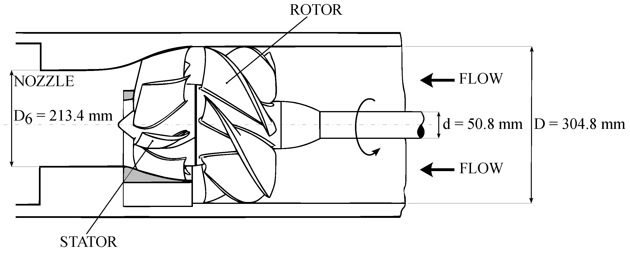
3.1. Case Geometry

The ONR Axial flow Water Jet (AxWJ-2) is a marine propulsion system based on the requirements of a military notional high-speed ship, the Joint High-Speed Sealift (JHSS) [56]. The core part of this waterjet system is the axial-flow pump, in which geometry and data are in the public domain to contribute to developing new designs and studies, such as investigations into cavitation. Pump prototypes have been scaled for model testing in three different facilities: the Naval Surface Warfare Center, Carderock Division (NSWCCD) 36-inch water tunnel, the Rolls Royce Hydrodynamics Research Centre (HRC) pump loop, and the John Hopkins University (JHU) water tunnel. In particular, the geometric configurations and results of the NSWCCD tests, reported by Chesnakas et al. [51], are taken as a reference for the present CFD study. The NSWCCD water tunnel has a recirculation system that allows the facility to operate as a pump loop. The pressure in the tunnel can be varied to study the pump’s behaviour under cavitating conditions, and the flow rate is controlled through a tunnel impeller. The AxWJ-2 test model (Figure 1) consists of a six-blade rotor housed inside a cylindrical casing with a diameter D = 304.8 mm and a tip clearance equal to 0.5 mm. The flow is then expanded through a nozzle equipped with an eight-blade rectifier stator. The latter is flanged at both the ogival hub and the shroud, which smoothly transitions from the rotor size to the throat diameter ( D 6 = 213.4 mm) using a revolved spline outline.

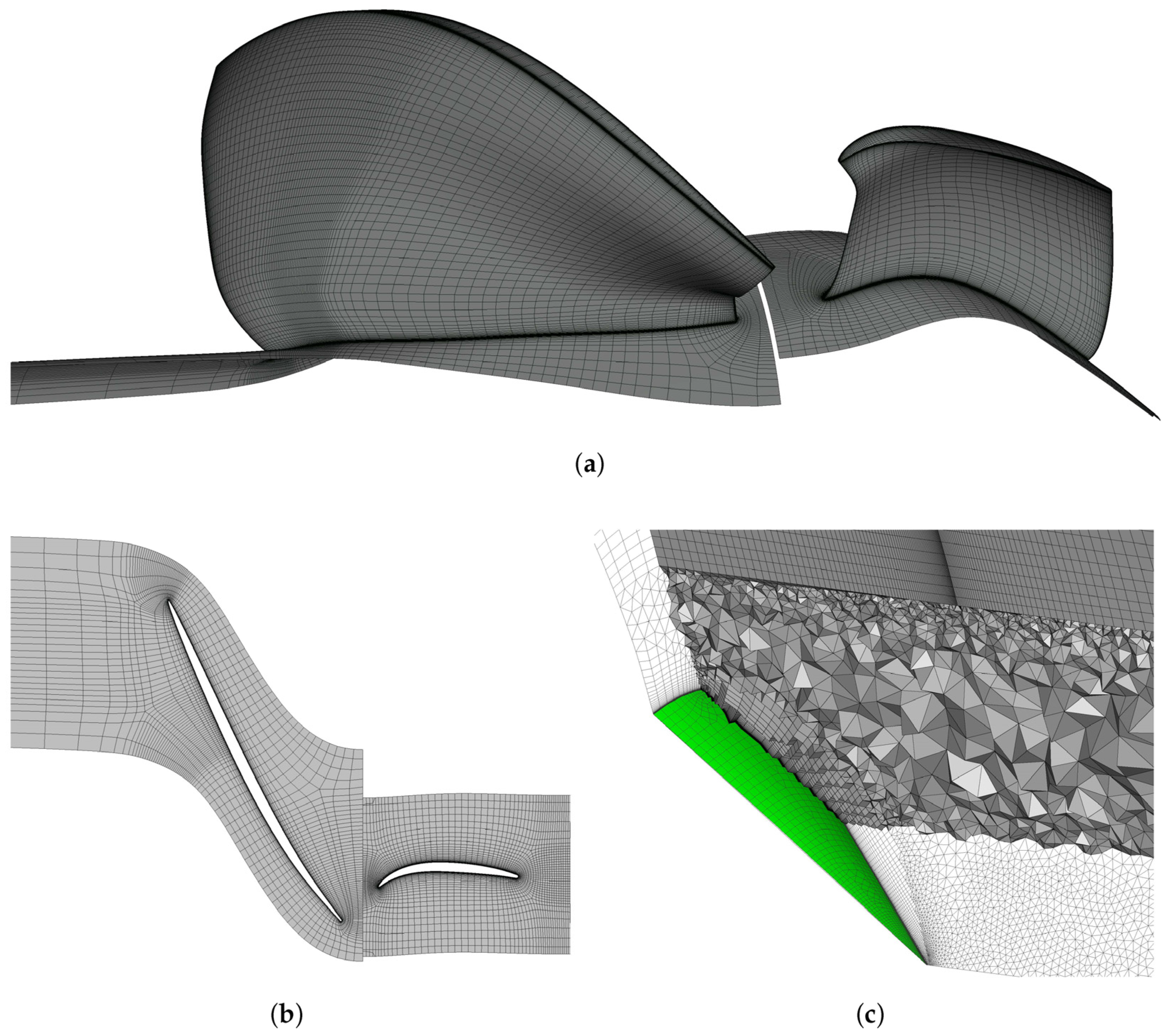
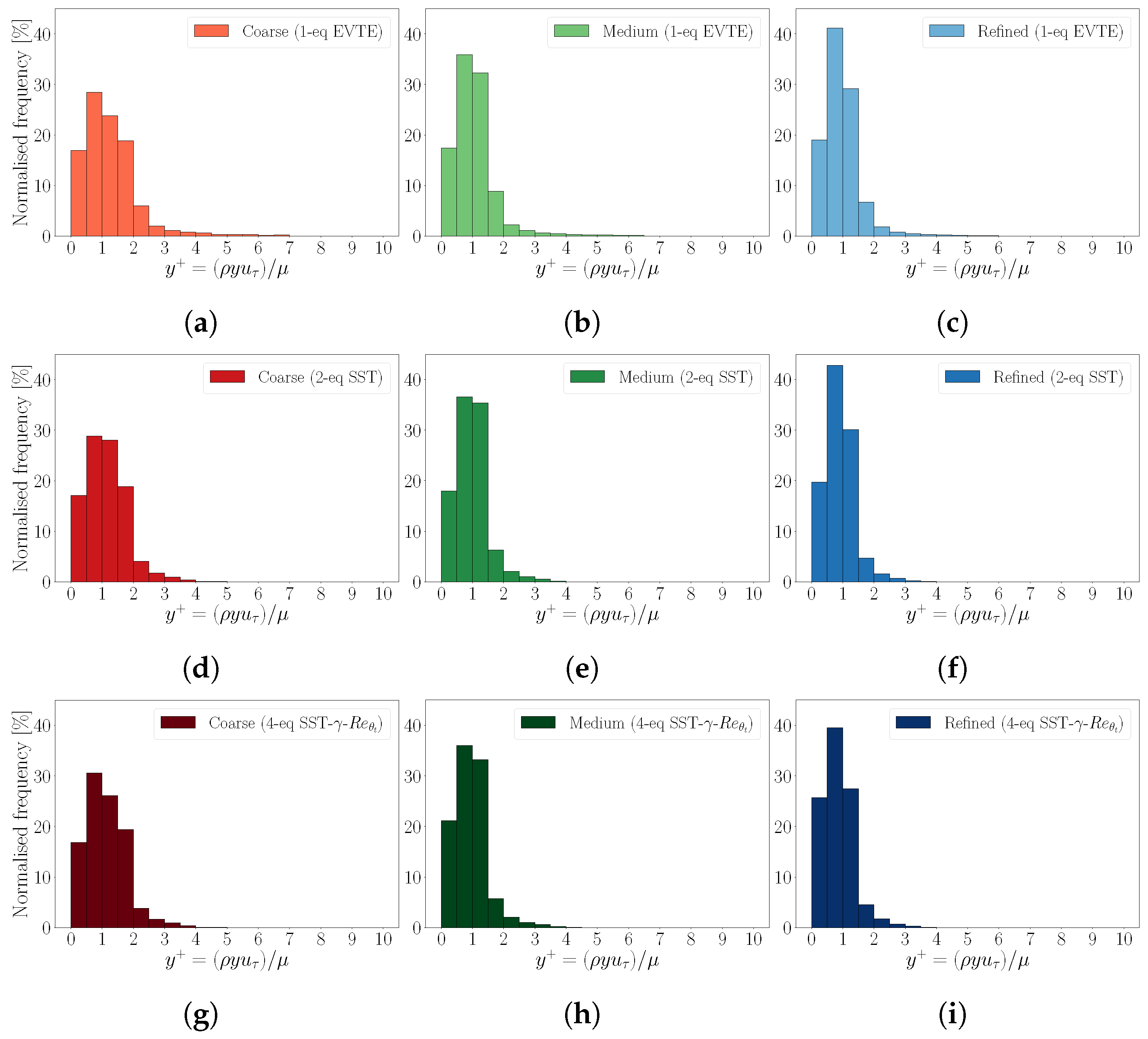
3.2. Mesh Generation

The computational domain is built following a multi-block strategy (Figure 2). Fully structured grids are generated for a single passage around the blade regions, using ANSYS TurboGrid® Figure 2a. The cylindrical inlet is included in the rotor domain, thus extending the inflow boundary 2 D upstream. The stator mesh is generated in the neighbourhood of the blade to exclude the cone nose and, then, to favour the cells’ quality. The discretisation approach is based on a target node count, which facilitates the control over the domain size required for the sensitivity study. The initial cell spacing from the regions of the wall, end walls, and blade surfaces included is chosen based on the inlet relative Reynolds number and set to match an estimated value of the y + ranging from 1.3 to 1.1 over the three refinement levels. Similarly, the maximum elements’ length expansion rate never exceeds 2.1. The nodes distribution is adjusted in order to provide an accurate discretisation of the rounded leading and trailing edges without affecting the quality of the surrounding cells Figure 2b. In terms of the rotor blade, a tip clearance of 0.02 inches is modelled. Here, the grid expansion rate is set to match the cell sizes at both the shroud and blade tip surfaces. A third block is generated using Pointwise® to further extend the domain 4 D downstream and include the hub’s sharp end. In this case, the grid is further divided into two regions. The first major one is created as a structured block, expanding radially from the shroud boundary towards the revolution axis. Then, the domain is completed with a hybrid meshing technique. Here, the remainder of the volume is filled with a combination of hexes, tets, prisms, and pyramids with normally extruded cells over the hub nose wall (Figure 2c). Expansion rates and initial cell spacing are set to match those of the communicating outflow boundary of the upstream stator block.

3.3. Numerical Schemes and Boundary Conditions

Steady-state simulations are conducted using Ansys CFX, which implements a node-based Finite Volumes (FV) approach. Advection and turbulence terms are discretised using a high-resolution scheme, which blends between a first-order and a second-order accuracy depending on the local values of the field gradient.
Concerning boundary conditions, the axial symmetry of the configuration allows for reducing the computational cost of the solution. Thus, rotational periodicity is enforced along the boundaries defining the blades’ channels, thus solving for the circumferential evolution of the flow in the missing portion of the domain. Then, the total pressure is imposed as the rotor inlet boundary condition, while the mass flow rate is set on the domain outlet. Solid regions are treated as no-slip walls. As a steady configuration, the interpolation of the field solution between the rotating frame and the stationary one is performed by adopting a mixing plane strategy. While on the matching sides between the stator and the exhaust, resulting from the multi-block strategy, a none-type interface can be chosen since neither pitch change nor frame change occurs.
For either nominal operation or thrust breakdown analyses, computations are initialized using single-phase solutions. In any case, the convergence strategy is kept unchanged whether the fluid is considered a pure liquid or a mixture. In particular, the stability of the solution is initially enhanced by running a maximum of 200 iterations with a local timescale approach, performed with a factor equal to 5. Then, the solution advancement switches to an auto timescale technique, with no changes applied to the default step computed by the solver. Here, iterations are stopped at a maximum number of 500. The hydraulic efficiency is monitored throughout the run as an additional stop criterion. In particular, that statistic’s Standard Deviation (SD) is evaluated over a moving interval of 40 iterations. Interruption of the computation is then determined by a value lower than 1 × 10 3 . Equations mass imbalances are always lower than 1%.
Simulation loops were conducted using a four-node cluster, with each node utilizing 10 computing cores equipped with Intel® Xeon® Silver 4114 CPUs @ 2.20 GHz. Convergence was achieved in less than 5 h for the most demanding configuration, which involved a fine grid at fully cavitating conditions. On average, cavitation model sensitivity analysis required approximately 2 h for each simulated point.

4. Model Tuning and Validation

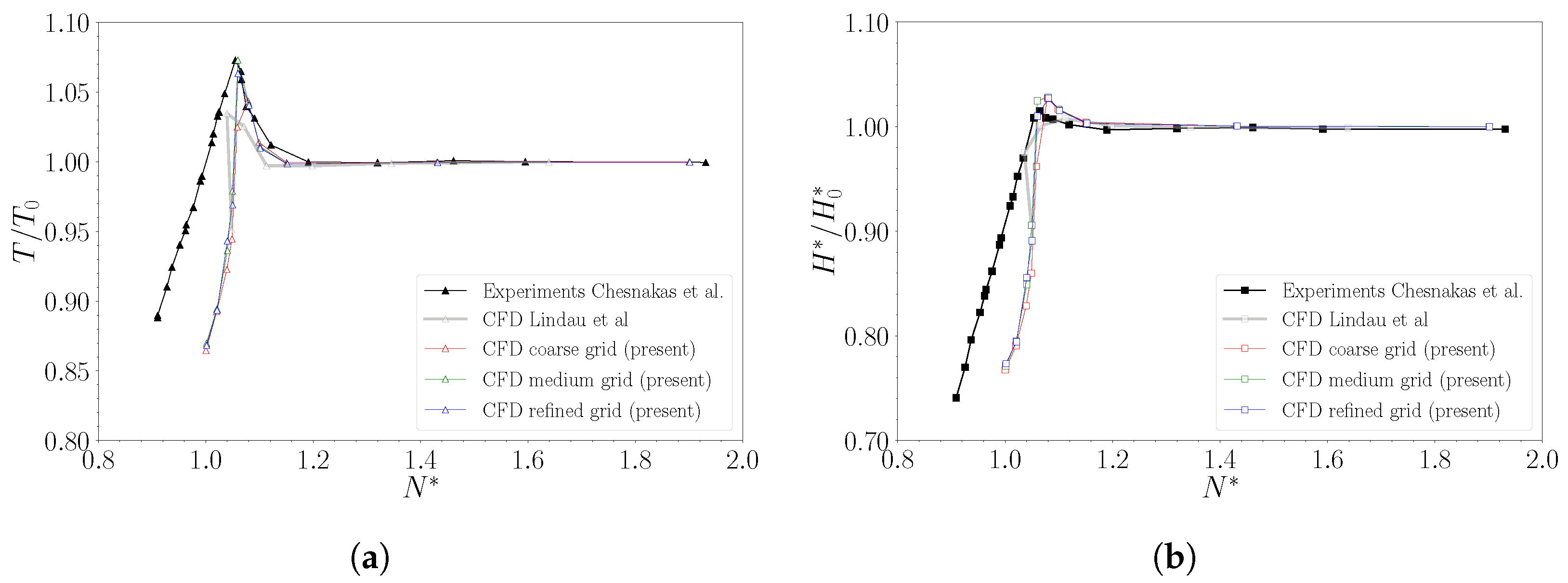
4.1. Global Parameters Analysis

A typical solution obtained with the present model is depicted in Figure 3. Here, the flow field distribution is reported through single-channel streamlines, superimposed on the static pressure contours over the pump’s wall surfaces. As can be clearly observed, the pressurised flow leaving the rotor blades is re-oriented by the stator along the axial direction. This action allows for optimal exploitation of the expansion for an axial thrust component generation.
In light of selecting the most suitable numerical arrangement, standard best CFD practices are followed [57,58,59,60]. Thus, the system flow dynamics is initially assessed by comparing the pump statistics under non-cavitating conditions between computations and measurements from Marquardt [61]. Following the tests procedure, simulations are conducted at a fixed rotational speed ( n = 1400 rpm) by varying uniformly the mass flow rate, controlled through the non-dimensional flow coefficient Q * = Q J / ( n D 3 ) , with Q J being the volumetric flow rate and n the rotational speed in rpm. The flow coefficient ranges from 80% to 112% of the design condition with constant variations Δ Q * = 0.034 . As regards the inlet total pressure, the value is set to avoid cavitation inception, based on the evidence by Chesnakas et al. [51]. Three parameters are used as metrics for the pump performance, namely: the head coefficient, H * , the power coefficient, P * , and the hydraulic efficiency, η . The latter are defined as follows:
H * = p t 6 p t 3 ρ ( n D ) 2
P * = 2 π n T ρ n 3 D 5
η = Q * H * P *
Here, p t 3 and p t 6 correspond to the total pressures at the inlet and outlet stations, respectively, whose values are computed at the measurements locations, following Marquardt [61]. Rotor torque is denoted as T.
Three levels of increasing mesh refinement are produced: coarse, medium, and refined, counting n 3 = 1.37 , n 2 = 2.88 , and n 1 = 6.02 million cells, respectively, each evaluated with the three increasingly complex turbulence models. Thus, an almost constant grid refinement ratio is considered r 32 = ( n 2 / n 3 ) 1 / 3 = r 21 = ( n 1 / n 2 ) 1 / 3 1.3 . Figure 4 reports the comparison between experimental data and present numerical calculations concerning H * , P * , and η trends as a function of the flow coefficient, Q * . As the reader can see, the outcomes of the medium mesh are entirely superimposed over the finer arrangements. As a result, the denser model does not significantly increase computing costs for meaningful accuracy gains. On the contrary, a modest spatial resolution dependence may still be identified between the coarse and medium levels. In any case, the overall trend of the curves reveals that the model underestimates the torque applied on the rotor blade, but the head produced is relatively close to the experimental results. As a consequence, the hydraulic efficiency of the system is overestimated by as much as 1.4%.

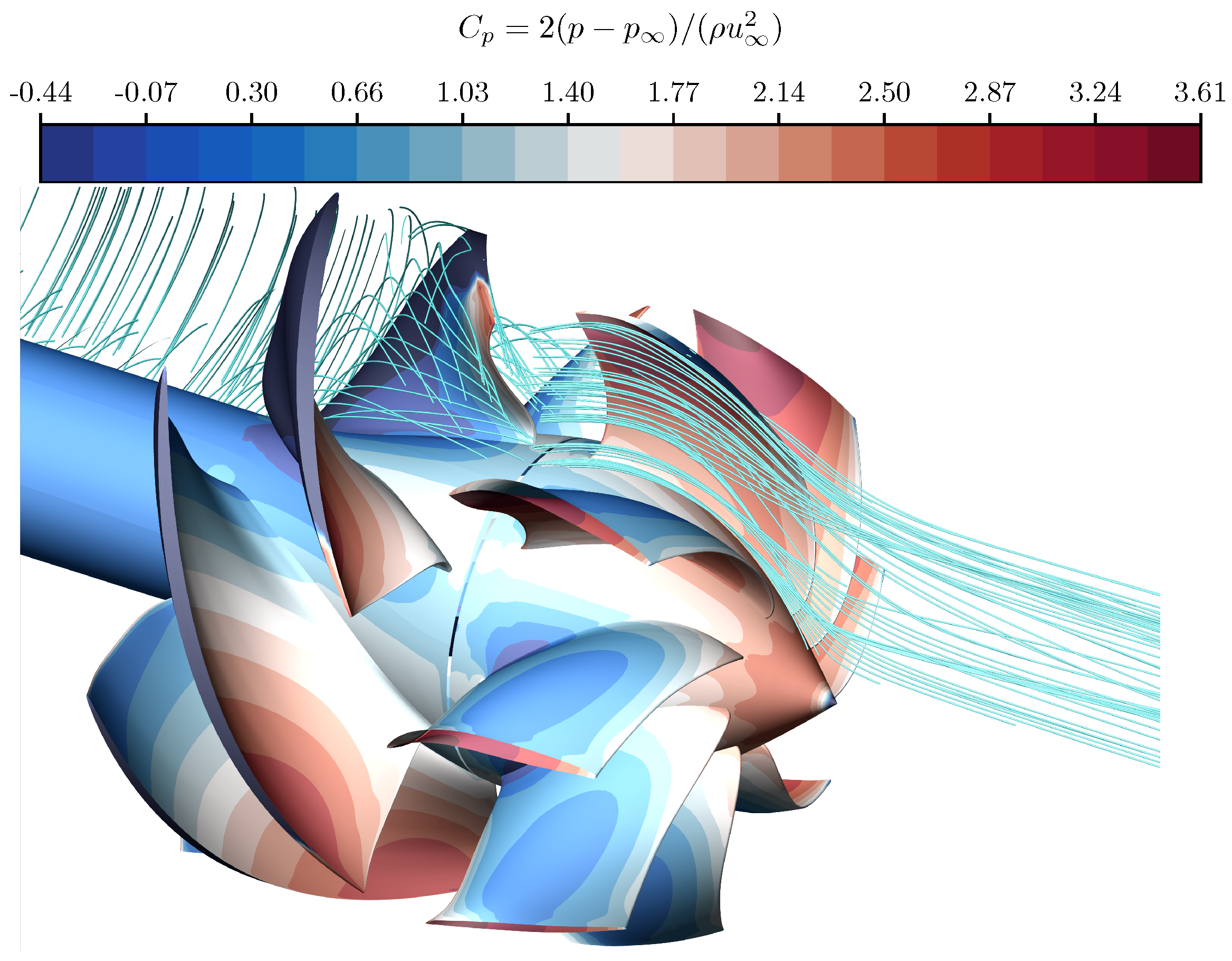
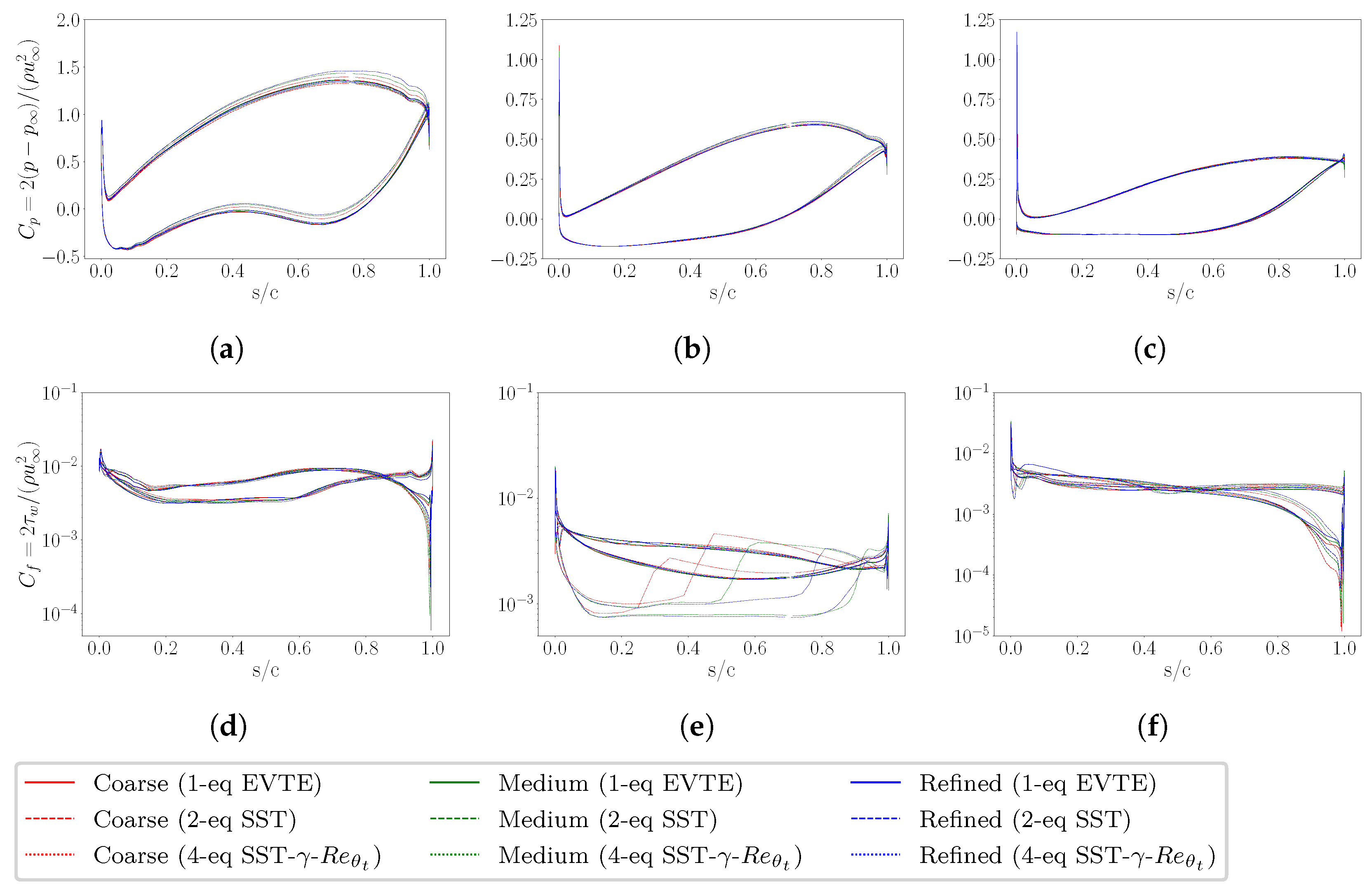
4.2. Local Parameters Analysis

As high-level qualitative metrics of the domain discretisation, the y + = ρ u τ y w / μ distribution over the rotor blade is analysed in Figure 5. Here, ρ and μ denote the flow density and viscosity, respectively, u τ = τ w / ρ is the wall friction velocity with τ w = μ u / y being the wall shear-stress, while y w is the first-off-the-wall cell distance. The results are reported for all the three turbulence models considered, i.e., EVTE (Figure 5a–c), k ω SST (Figure 5d–f) and TSST (Figure 5g–i). The latter are evaluated incrementally with the three refinement levels, respectively. Histograms show that, as the mesh becomes finer and finer, the y + distribution narrows around the median value, which is, in any case, lower than 1, thus denoting an accurate resolution of the boundary layer on the rotor surface. Especially from the medium refinement, and even more so at the finest one, the categories of values up to 1.5 gather almost 90% of the rotor cells.
Additionally to the y + distribution, the grid sensitivity at the local level is monitored by looking at the blade loading. The latter is studied by investigating the behaviour of either pressure and viscous stresses, through the streamwise distribution of the pressure and the friction coefficients, the latter holding as follows:
C p = p p 1 / 2 ρ u 2
C f = τ w 1 / 2 ρ u 2
Here, p and p denote the wall and the free stream static pressure, respectively, while u is the free stream relative velocity. Load coefficients are monitored along with the rotor surface for three distinct span locations, i.e., near hub, midspan, and tip (Figure 6), respectively. As regards the pressure coefficient, the three grids produce almost the same distributions with all the turbulence models, especially at midspan (Figure 6b) and tip (Figure 6c) where the curves are superimposed. Minor discrepancies can be spotted for the hub section (Figure 6a), instead. Here, the discretisation is more effective on the elements’ quality due to the local gradients generated by the curved hub shape. In terms of viscous shear, the discussion holds almost true. In fact, any configuration of refinement and turbulence model recovers essentially the same wall-flow distribution at the hub (Figure 6d) and shroud (Figure 6f) blade sections. The situation slightly differs at the midspan (Figure 6e).
Here, indeed, the main discrepancy is due to the enhanced ability of the TSST to detect the laminar-to-turbulent transition point [55]. This effect marks a substantial physical difference compared to the other two models, which solve the flow almost equally. Consequently, the entire load distribution is affected, and it is clear that such a distinct equations formulation will never let the solution be insensitive to the closure technique. In this regard, it should be noted that the two extreme span sections depict no discrepancies connected to transitional behaviours. This fact is explained since the corresponding flow evolution is deeply affected by the casing boundary layer, which mitigates the typical development detectable at midspan, where the blade section is more relatable to an aerofoil in free stream conditions.
Finally, the Grid Convergence Index (GCI) [62] has been employed over a case in fully cavitating conditions to evaluate the effects of the grid discretisation error on the cavitation prediction. In this regard, the application of the method is based on the selection of two quantities, commonly referred to as φ k , k being the refinement level. Here, these are chosen as local and integral cavitation-related variables: the estimated SS vapour bubble length, l B , and the normalized volume of vapour on the pump domain, V v a p , respectively. In particular, l B is measured as the normalized streamwise distance between the two locations on the blade surface at which α v = 0 , while V v a p sums up the cells volume where α v > 0.1 and is then normalized with the coarse grid result. GCI parameters for both medium ( G C I m e d i u m 32 ) and fine refinement ( G C I f i n e 21 ) are summarised in Table 1. These include the extrapolated variables, φ e x t , and error, e e x t .
Based on the model tuning and validation findings, the authors agree that the medium resolution provides an optimal balance of accuracy and computational cost. As far as the turbulence modelling, the previous results suggest that no particular advantage can be obtained when selecting the one-equation EVTE instead of the two-equation SST. Therefore, in this regard, the choice is guided by the trusted published studies available in the literature [34,36,37,38,39]. As a result, subsequent investigations of the system under cavitation conditions have been performed using this numerical configuration.

5. Results and Discussion

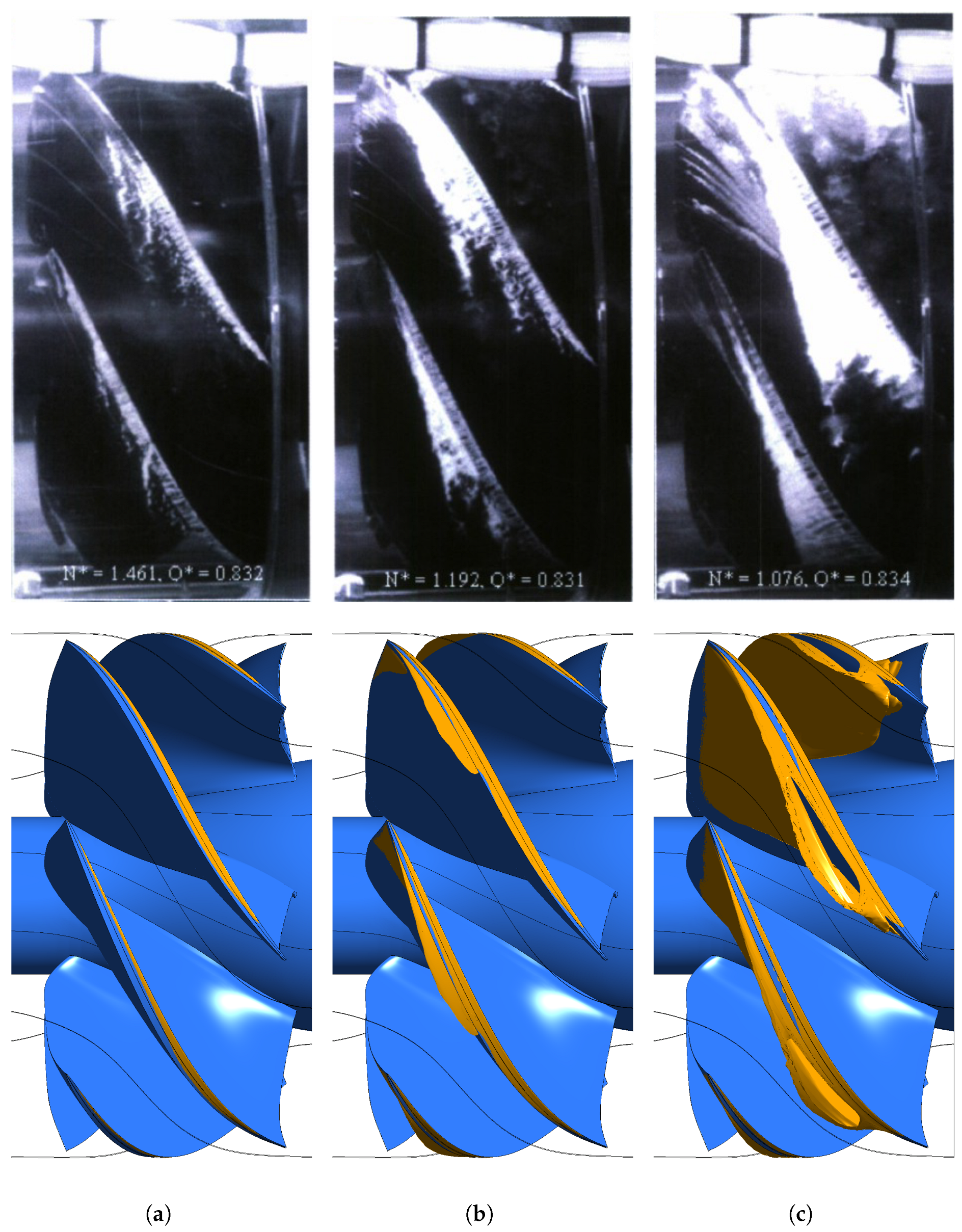
5.1. Thrust Breakdown Numerical Assessment

Upon validation of the numerical model, the system behaviour under cavitation conditions is first investigated through thrust breakdown simulations, and then compared with available experimental and numerical results (Figure 7). Following the test procedure outlined in Chesnakas et al. [51], the total pressure at the inlet is gradually decreased while keeping the flow rate constant at Q * = 0.83 . The decrease in pressure is expressed through the non-dimensional cavitation coefficient, defined as:
N * = p t 3 p v ( ρ n D ) 2
where p v is the water vapour pressure. During loops computations, the rotor’s angular velocity is set to n = 2000 rpm. The reported values are normalised with corresponding parameters, H 0 * (Figure 7a) and T 0 (Figure 7b), obtained at non-cavitating conditions ( N 0 * = 3.283 ). As can be seen from the trends in the test data, both torque and head coefficient tend to increase in the early stages of cavitation until about N * = 1.06 . As reported by Tan et al. [12] and Chen et al. [13], at this phase of flow evolution, part of the suction side of the rotor blade is covered by cavitation, so the pressure is close to the vapour pressure. Instead, the Pressure Side (PS) is still unaffected by cavitation. Thus, even if the pressure in the blade passage decreases, the partial cavitation in the SS leads to an increase in the blade loading and, thus, to augmented work performed by the pump. Performance curves depict a remarkable ability of the numerical model to recover such operating conditions, even when compared to other CFD results. The torque ramp-up phase is almost superimposed on the experimental curve, except for a minor offset in the very initial portion. This behaviour holds for the three refinements; however, a significant difference can be identified in the predicted value of the peak load, especially when comparing the coarse level with the finer ones. At this condition, the refinement allows for a reduction of the error from >4% to <1%. This effect originates from an earlier prediction of the cavitation breakdown. As regards the head coefficient, it can be observed that the model behaves differently from what is discussed above for nominal conditions. Here, the energy released to the fluid is overestimated almost throughout the beginning phase. As a result, the peak condition is higher than measured and almost mesh-independent, with the error being in any case restricted around 1%. As N * keeps decreasing and the values of T and H * start dropping steeply, the numerical model deviates significantly from the test data. A similar trend can be observed in the CFD results reported in the study of Lindau et al. [32]. The reasons for this behaviour were first adduced by Chesnakas et al. [51] and later confirmed by Tan et al. [12] and Chen et al. [13]. In fact, lowering the inflow pressure for the breakdown test caused tunnel impeller cavitation which, in turn, reduced the circulating mass flow rate. Consequently, breakdown values from measurements were normalized using the performance values obtained at the corresponding flow coefficient in non-cavitating conditions. Therefore, discrepancies in the numerical results should be ascribed to two concomitant effects: the boundary conditions imposed do not reflect the flow conditions during the experiments, and, secondly, the reference values for the normalization are not adjusted according to the actual mass flow rate measured.
Figure 8 provides a graphical comparison between pictures of cavitation volumes in the tip region, reported by Chesnakas et al. [51], and isosurfaces of vapour volume fraction α v = 0.3 resulting from the present model. Figure 8a,b corresponds to low cavitation conditions confined at the blade tip, while Figure 8c shows the performance ramp-up phase preceding the thrust breakdown.
Flow visualization makes it possible to conclude that the model yields a vapour volume distribution comparable with the structures reported from experimental pictures, especially for attached sheets at the SS along the span. However, computations generally defect a proper reconstruction of the cavitation bubbles associated with the TLV, which is even more evident near the TE. This particular flow feature was analysed in detail in Guo et al. [37]. According to their work, the proper way to reconstruct the vortex requires unsteady simulations with a peculiar modification of the cavitation model. Such a level of attention to that structure is beyond the purpose of the present work. During the calibration phase, the model devised by Guo et al. [37] was tested. Within a steady computations approach, their modifications did not significantly improve the results obtained with the default cavitation model, and the investigation is not included here.

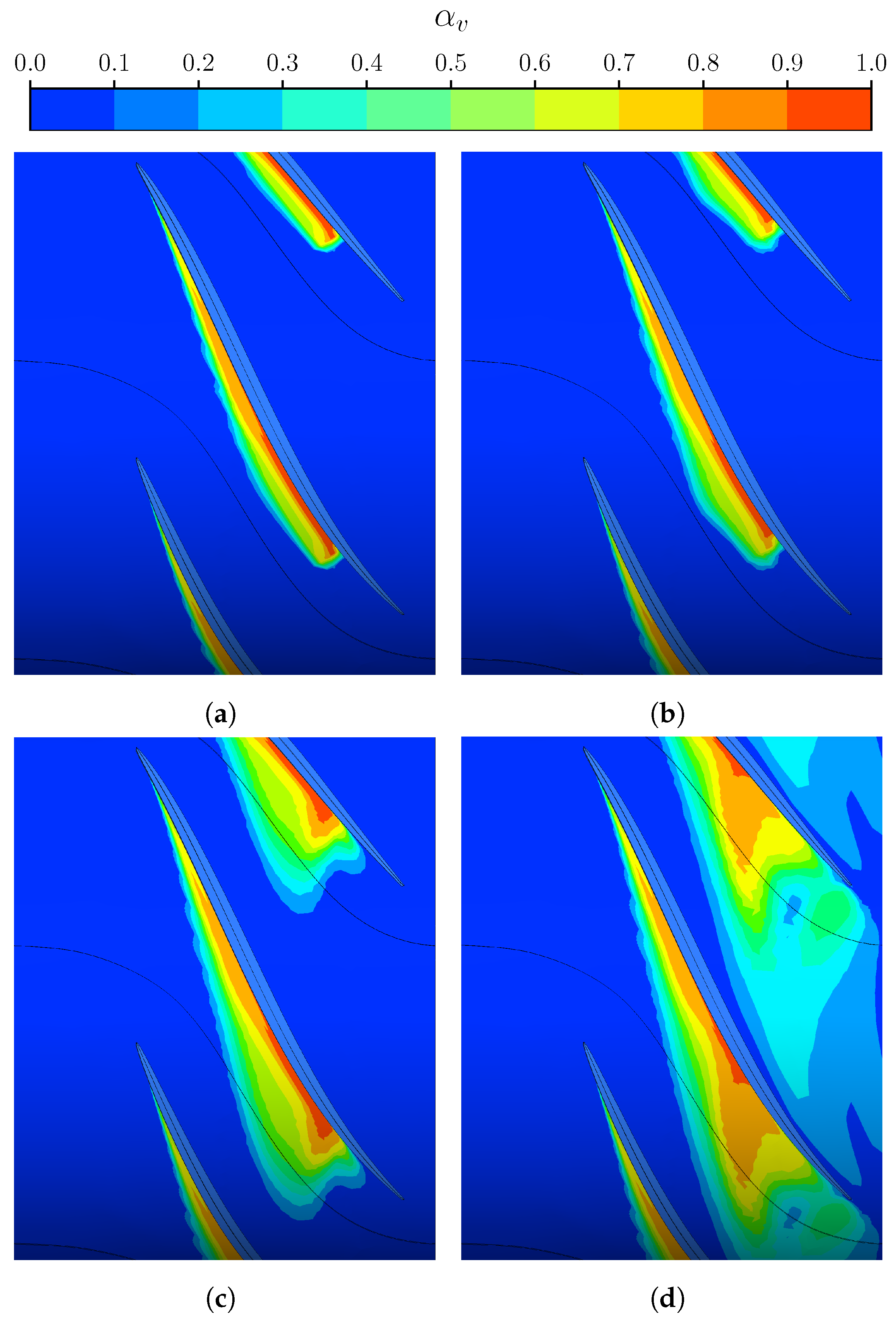
5.2. Cavitation Model Parameters Sensitivity

Based on the obtained results regarding thrust breakdown, it is evident that describing these phenomena numerically with the CFD model is challenging. Thus, the following analysis aims at tuning the cavitation model parameters to better match the experimental results. Specifically, several constitutive empirical coefficients are changed to evaluate the influence on the phase transfer within the fluid mixture. To track the influence of the parameters independently, each one is varied and discussed while keeping the others set at the default value. The discussion on each coefficient modification is carried out by looking at three different results: the vapour volume at the rotor tip, the load distributions on the rotor blade, and the pump performance as a function of N * . As regards the flow field information, the reported numerical solutions are obtained at an operating point with Q * = 0.83 and N * = 1.076 . The load distribution of the impeller, at span 99 % , is monitored through the pressure coefficient, C p . The latter is plotted as a function of the normalized streamwise direction s / c , ranging from 0 at the Leading Edge (LE) to 1 at the Trailing Edge (TE).

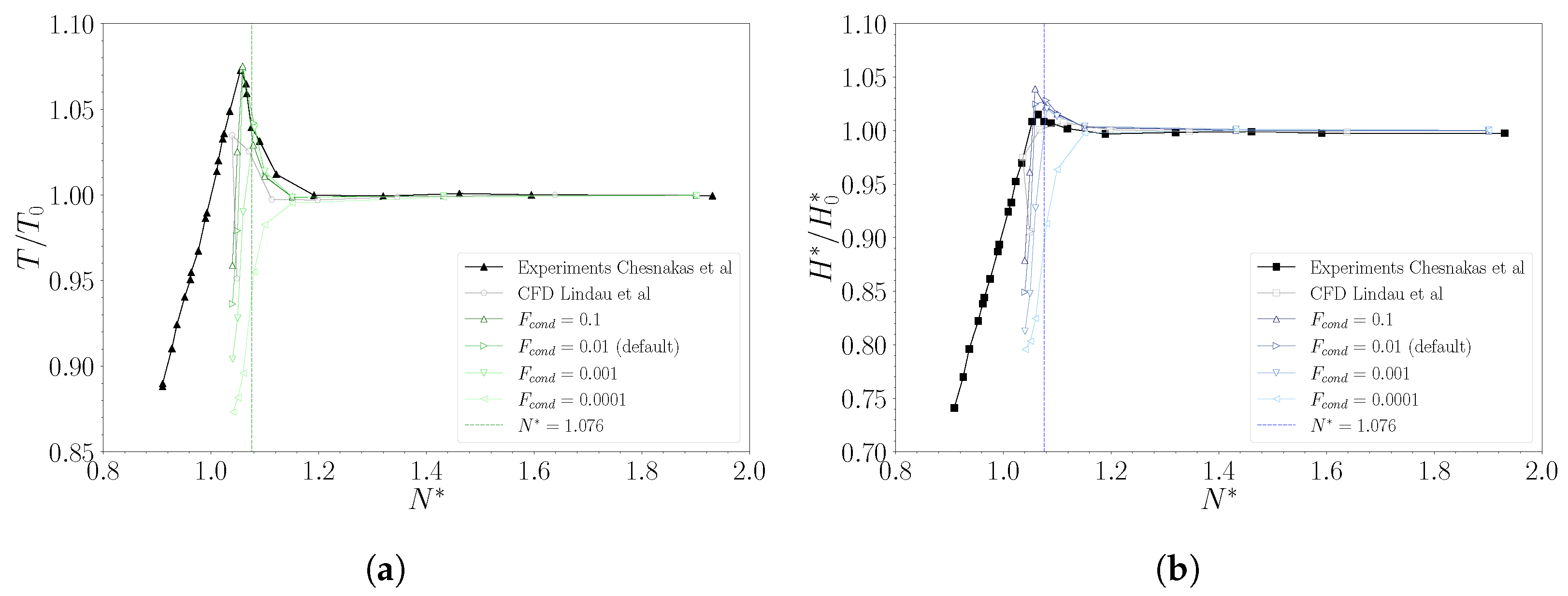
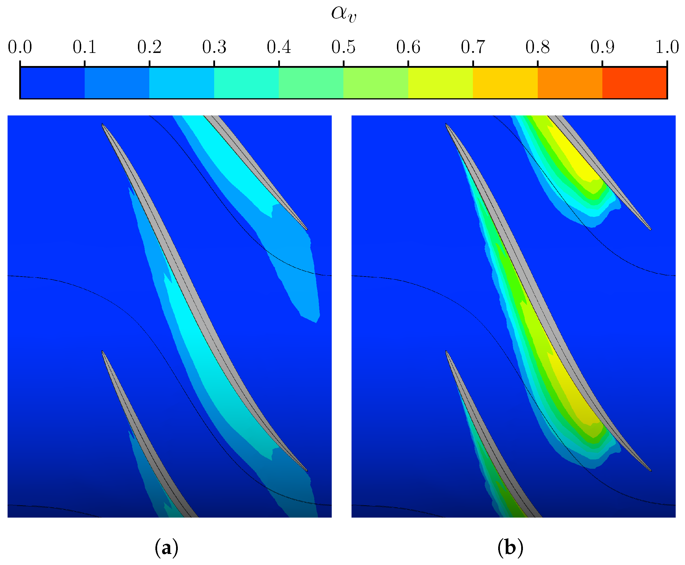
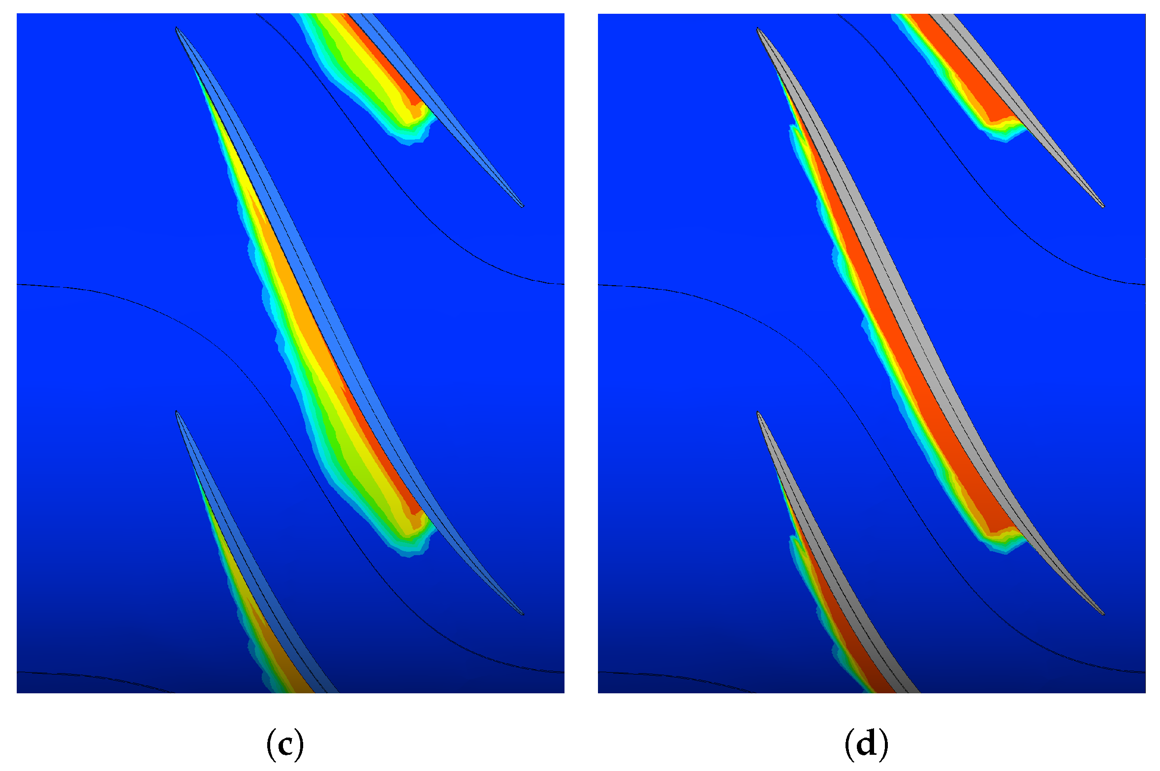
5.2.1. Condensation Coefficient

As expressed by Equation (12), the condensation coefficient, F c o n d , is an empirical factor that controls the mass rate of change from vapour to water at the interfaces where p > p v a p . Lowering this parameter smoothens the liquid phase mass transfer equation, which, as a result, promotes the extension of the vapour regions. This effect can be visualized through the contours of the vapour volume fraction over the blade tip in Figure 9. Here, the solution is computed at N * = 1.076 for each of the values considered for F c o n d , respectively: 10 (Figure 9a), 1 (Figure 9b), 0.1 (Figure 9c), and 0.001 (Figure 9d) times the default quantity.
Increasing the value of the condensation coefficient acts as a limiter for the distribution of the vapour region interface, which is restricted to a sharp region over the SS. In this regard, contours suggest that such a modification is less effective than the default value. This is further confirmed by the blade loading trend (Figure 10), where the curves at augmented and standard coefficients are almost superimposed. Conversely, by reducing the value of the same order of magnitude, the broadness of the vapour phase spatial distribution results significantly extended over the SS of the blade. Applying an additional lowering causes the vapour bubble to expand up to the PS of the adjacent blade. As a result, the flow in the blade passage is further obstructed, thus inducing an increment of the relative velocity that feeds the cavitation process again. This evolution justifies the non-linear behaviour of the flow development concerning the variation in the coefficient. At this stage, even the load on the PS of the blade is affected, resulting in a general decay of the shaft power. Admittedly, this condition is primarily determined by offloading the SS. Here, the pressure distribution transitions from an abrupt phase change to a gradual recovery as the mass transfer is smoothed by the condensation coefficient decrement. Consequently, the extension of the pure vapour region augments as F c o n d , while, oppositely, the field is dominated by the mixture with limited portions at unitary volume fraction. Additionally, the blade loading reversal that can be observed near the trailing edge is reduced together with the ending value, further affected by the mixing with the partially vaporized wake.
As the inlet pressure drops throughout the breakdown loop, the increased amount of vapour generated by the lower values of the condensation coefficient is responsible for a significant discrepancy between measured and predicted performance (Figure 11). In fact, the enhanced cavitation effect leads to an anticipated drop in machine statistics. Consequently, the predicted curves depart from the experimental ones much more as F c o n d decreases, and only for the highest values is the peak performance in good agreement. In particular, this consideration holds for the shaft power (Figure 11a), while, in contrast, the head coefficient (Figure 11b) is again in excess, despite corresponding in terms of N * .
As regards the flow evolution at full breakdown conditions, the model depicts the same behaviour as that discussed in the previous sections, where the mismatching between the imposed and tested mass flow rate is the principal responsible for the overestimated steepness of the performance decay.

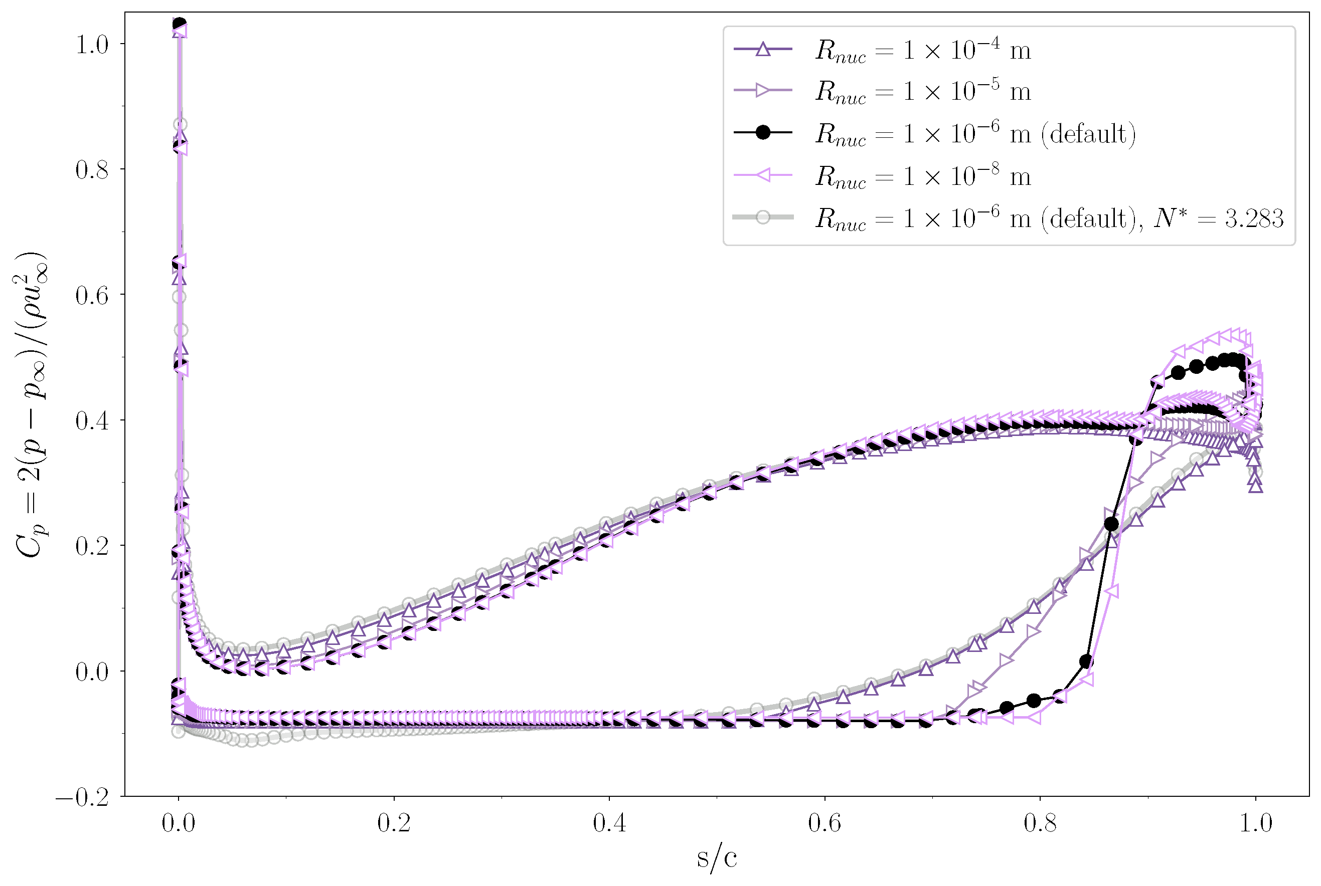
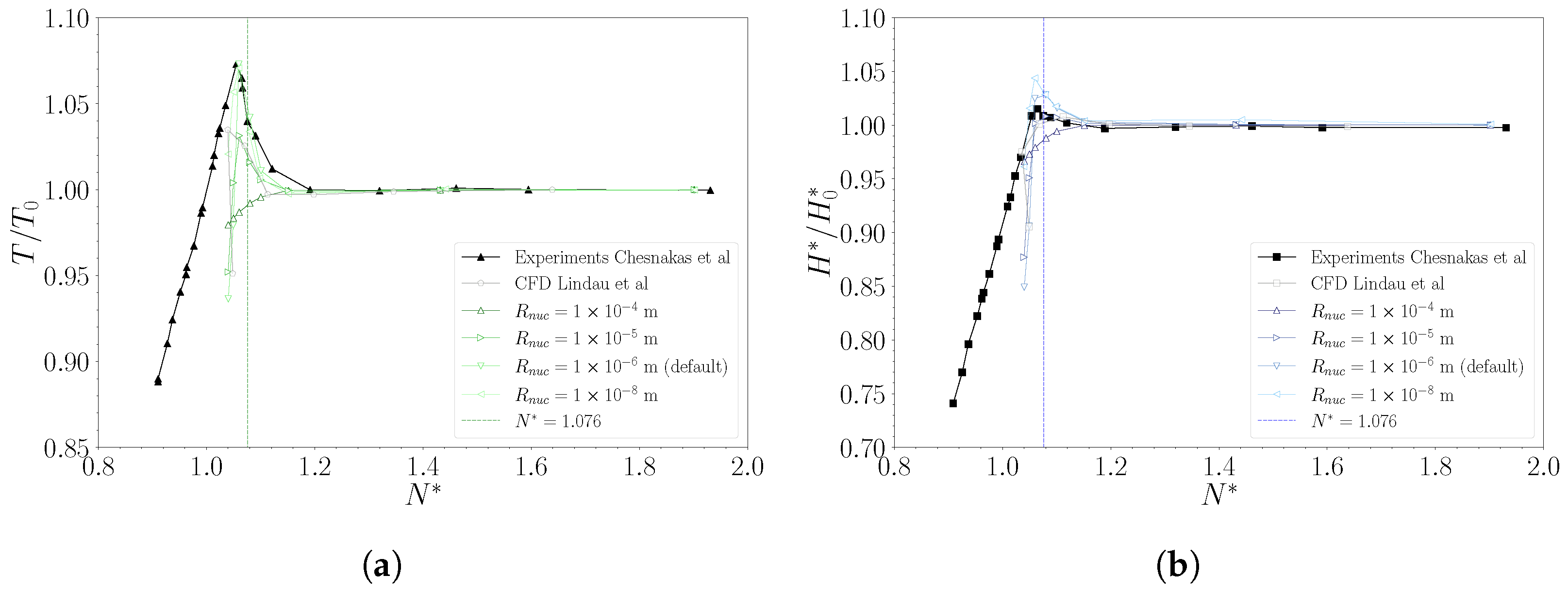
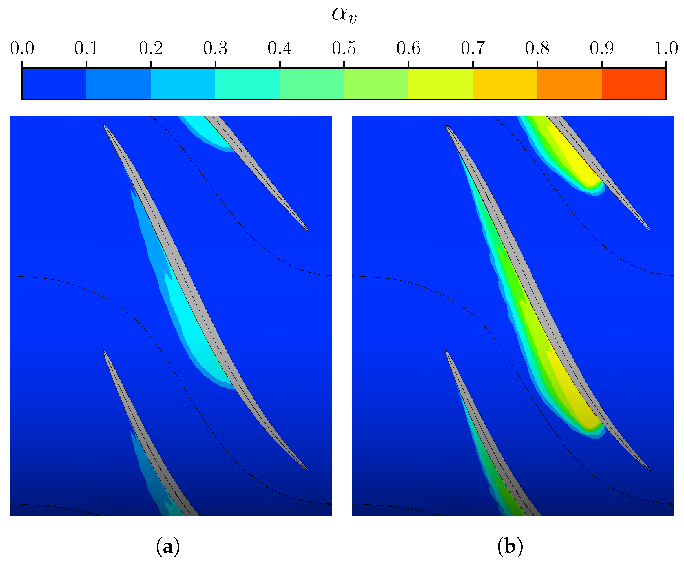
5.2.2. Nucleation Site Radius

Equations (11) and (12) suggest that decreasing the nucleation site radius enhances the mass rate of change. Consequently, this factor can strongly affect the phase transition of the flow during both evaporation and condensation processes (Figure 12). By smoothing the transport phenomena at the phase interface, the increase in R n u c tends to constrain the development of the cavitation bubbles. This results in more widely spread vapour regions, characterized by low values of the volume fraction (Figure 12a,b). Moreover, such a modification performs a backward shift of the cavitation sheet over the SS of the blade. The two-phase region inception moves upstream as the coefficient increases, with the consequent gradual departure from the trailing edge (Figure 12c,d).
This evolution follows a general reduction in the spatial distribution of the vapour fraction. In fact, as the mass transfers are promoted between evaporation and condensation, the local gradients of the phase change interface increase rapidly. Consequently, the transition is sharply delimited, resulting in a denser vapour concentration but confined to a much narrower region.
This flow development through the blade passage has an evident impact on the rotor loading (Figure 13).
Although the effect on the vapour volumes is similar to the results discussed in the previous section, the pressure field depicts some different outcomes. In fact, as the cavitation region expands with the increasing coefficient value, the low vapour concentration is not sufficient to generate significant obstruction consequences. As a result, the pressure coefficient over the PS of the blade is not appreciably influenced, except for minor variations due to the aforementioned backward shift of the sheet. These fluctuations are more pronounced away from the mid-chord location, whereas all the curves are superimposed at that point. In general, as R n u c rises, the flow evolution tends to increase the loading in the fore half of the blade and, contextually, to reduce it towards the aft. While considering the behaviour on the SS, pressure coefficient curves show a similar trend as that observed earlier. As the mass interchange between the two phases is promoted, the cavitation volume tends to develop over a more extended portion of the blade but with a reduced extension on the passage. In this condition, the sharp interface is again clearly depicted by the sudden excursion of the C p towards the TE, where the flow mixing at the wake occurs after a limited region with a load reversal. Figure 14 reports the evolution of the pump performance throughout a breakdown loop. Here, the effect is similar to what is discussed above. In fact, as the model coefficient variation is responsible for an extension of the vapour volume, the statistics drop occurs at higher values of the cavitation parameter N * . However, since the sensitivity does not affect the general shape of the curve, an earlier breakdown corresponds to reduced hydraulic peak performance in either torque (Figure 14a) and head (Figure 14b). Again, improved accuracy in the predicted value of the former goes hand in hand with an underprediction of the latter. Consequently, by reducing the value of R n u c , the rotor peak load matches experimental measurements with a gradual insensitivity to the modification factor. Conversely, the pressure rise estimate shows a remarkable agreement when the nucleation site radius is increased by one order of magnitude. In fact, this variation allows for reducing the relative error of all the points corresponding to the initial breakdown phase, from a maximum of >9% to about 5%. However, this results from a reduced rotor loading and confirms the model’s tendency to overpredict the pump’s head rise capability. This behaviour shows a specific dependence on the flow evolution of the TLV (Figure 15). In fact, an increased value of R n u c to 1 × 10 5 (Figure 15c), when compared to default conditions (Figure 15a), seems to generate a vapour distribution that better approximates the one captured during experiments (Figure 15b), especially at the blade’s tip, which relates to the improved prediction of average total pressure. On the other hand, the entire blade surface experiences a load reduction. As a result, the model benefits no enhancement in terms of efficiency estimate, which remains higher than measured values. However, this result stems from the adjustment of a parameter that impacts both condensation and vaporization processes. This evidence suggests that enhancing accuracy may involve a combination of coefficient alterations.

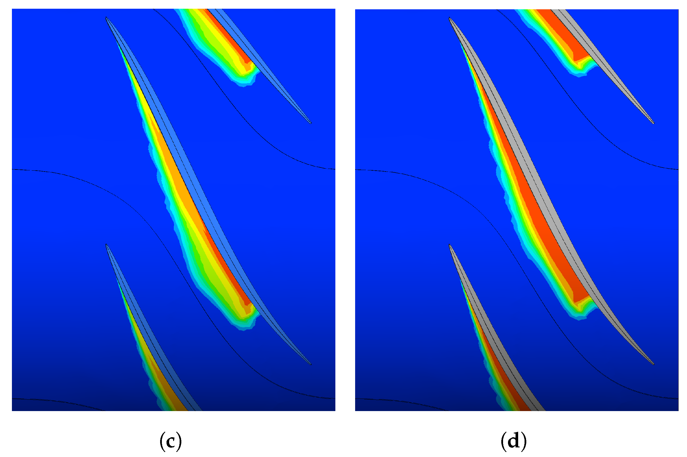
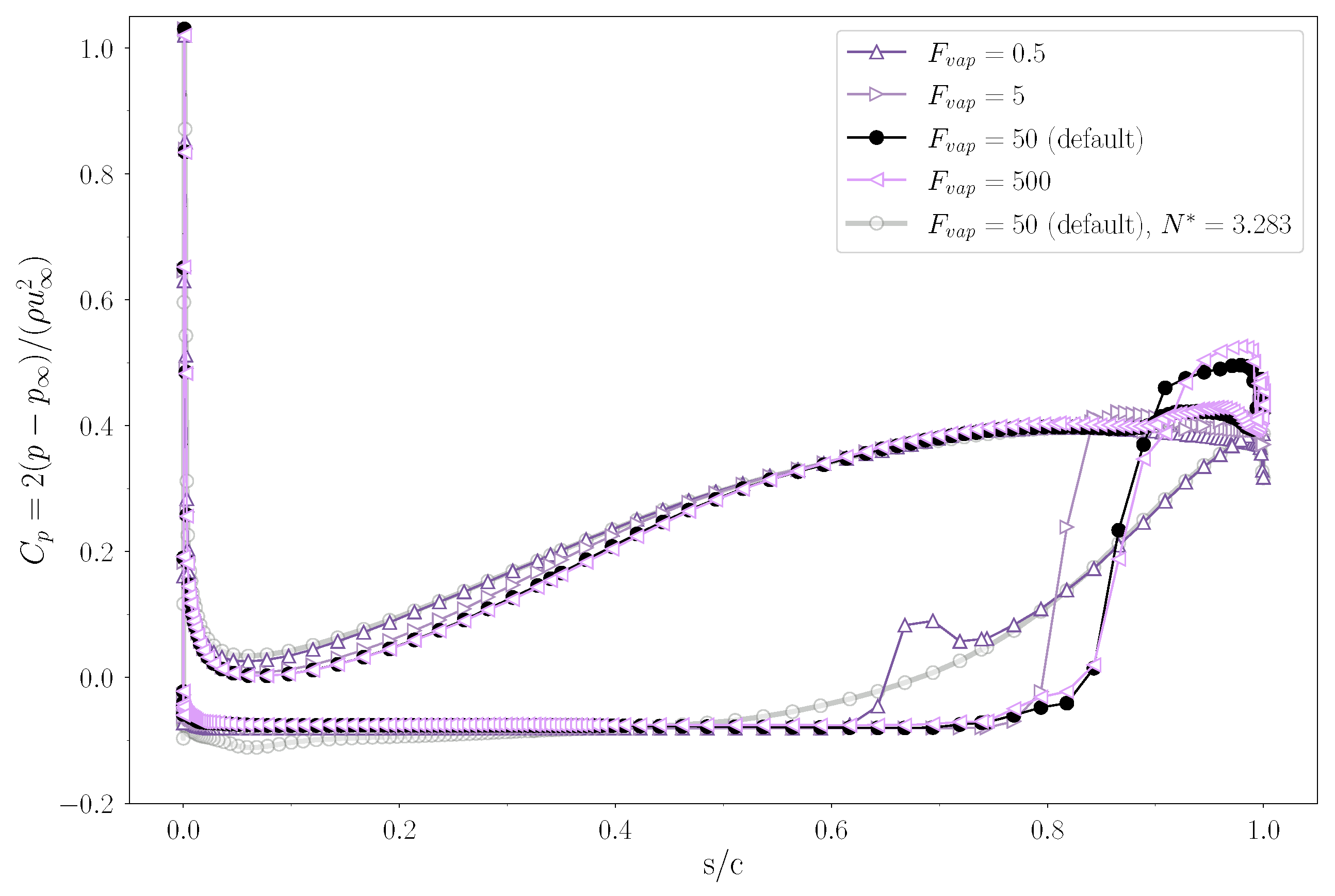
5.2.3. Vaporization Coefficient

The vaporization coefficient is another fundamental parameter for calibrating the ZGB cavitation model. According to Equation (11), this factor regulates the phase transition from the liquid to the vapour state, which is responsible for the interface phenomena occurring at cavitation regions where p < p v . In particular, lower values of F v a p constrain the mass transfers towards the vapour phase, thus acting as a limiter for the vaporization process. The vapour field distribution is reported in Figure 16. In this case, the coefficient variation’s impact depicts a different trend. In fact, as the value is enlarged from two (Figure 16a) to one (Figure 16b) order lower, and then to one order greater (Figure 16d) than the default (Figure 16c), both vapour generation and extension are promoted.
Consequently, as the bubble expands within the blade channel and over the SS, the gas concentration and the interface sharpness increase; this aspect significantly changes the model’s behaviour if compared with the discussions in the previous sections.
Concerning the pressure distribution (Figure 17) near the blade tip walls, the trend on the SS is similar for the region up to location 0.6 in normalized streamwise coordinates. Here, the curve for F v a p = 0.5 abruptly departs with a sudden increment that is quickly arrested. Then, the mixing at the TE is reached with smoother progress. Conversely, blade loading assumes a barely appreciably different distribution by reducing the coefficient by a single order of magnitude. In fact, except for a slightly lower extension of the vapour region, the phase transition is sharp as the curve obtained with default conditions. For larger F v a p values, the curve resembles the reference curve, both showing a reversed load on the segment of the constrained terminal blade. Again, the PS shows minor dependency on the cavitation behaviour, except for a limited region before the mid-chord, where a slight pressure excess (compared to the reference curve) quickly mitigates as the coefficient increment brings again F v a p towards values closer to the default one.
The above observations affect the pump performance throughout the breakdown loop (Figure 18). The constraint set by reducing the vaporization coefficient on the vapour generation process delays the development of the cavitation bubble. Consequently, the rotor can tolerate lower inlet pressures; therefore, the statistics peak and related drop shift toward smaller values of N * . The lowest coefficient considered, F v a p = 0.5 , performs an evident flattening of the peak performance. This effect causes the curve to remain almost unchanged as the cavitation coefficient decreases. On the contrary, the increasing trend typical of the initial cavitation stages is so sustained that torque (Figure 18a) and head (Figure 18b) decay appear well beyond the simulated values of N * .
Regarding the other parameters considered, no significant influence can be detected on the performance values. Instead, the curves only shift to the left, indicating peak performance at lower inlet pressure values. This aspect confirms a dependency on the vaporization coefficient that is highly non-linear, denoting substantial differences when changing from 0.5 to 5 while, in contrast, for higher values, the variations are minimal. This analysis confirms that the model is independent of F v a p for values more significant than the default, which holds in a wide range of operating conditions.

6. Conclusions

The present work investigates the tuning of a cavitation model applied to the flow evolution of a propulsive axial-flow pump, aiming to fill the deficiency of comprehensive studies on complex systems’ off-design operations. Thus, steady-state Reynolds-Averaged Navier–Stokes (RANS) equations are solved over a single rotationally periodic passage of the rotor-stator assembly, and the results are compared with available experiments. Modelling of turbulence terms is first analysed through three different formulations, based on the number of closure equations, respectively: the one-equation Eddy Viscosity Transport Equation (EVTE), the two-equation k ω SST and the four-equation Transition SST. Based on considerations in terms of accuracy and computational costs, the second model is chosen to conduct the cavitation model sensitivity. The latter involved the systematic variation of the empirical parameters defining the Zwart-Gerber-Belamri (ZGB) formulation of the phasic mass transfer within a homogeneous fluid approach.
Primarily, the pump’s performance is compared with the available experimental data, at either nominal and thrust breakdown conditions, using the cavitation model with default configuration. In this regard, grid dependency analysis is not effective in mitigating the tendency to overestimate the system’s hydraulic efficiency. This overestimation arises from torque underprediction during nominal operations computations and, conversely, from pressure rise overestimation during breakdown loops. To further investigate this discrepancy, the medium-refined grid was retained and cavitation model sensitivity was evaluated through variations in the condensation coefficient, the nucleation site radius, and the vaporization coefficient, by applying multipliers ranging from 10 2 to 10 (up to 10 2 for the second quantity) to the default values. In fact, manipulation of these parameters allows for direct control of the phase transfer mechanisms. The outcomes evidenced that linear variations in the multipliers’ order of magnitude result in non-linear responses of the flow behaviour. In fact, when modified to promote vapour generation, the condensation coefficient and the nucleation site radius show a similar tendency to extend the bubble into the blade passage and, contextually, reduce the vapour concentration. On the contrary, the vaporization coefficient regulates, in the same way, both the bubble size and concentration. However, although torque reconstruction still represents a limit of the model, applying a factor 10 to the nucleation site radius default value allowed for reducing the maximum error of the head rise near breakdown of 4%
Considering the improvements achieved by altering the nucleation site radius, which has an impact on both condensation and vaporization processes, future investigations are planned to consider the effects of combined variations of the coefficients. In addition, since this study constitutes a part of a major endeavour regarding the propulsive performance of installed pump configurations, proper numerical model calibration will be spent in characterising the mutual interaction between the machinery itself and the propelling casing.

Author Contributions

Conceptualization, F.A., F.D.V. and A.B.; methodology, F.A., F.D.V. and A.B.; software, F.A. and A.B.; validation, F.A. and A.B.; formal analysis, A.B.; investigation, A.B.; resources, F.A. and E.B.; data curation, A.B., F.A., F.D.V. and E.B.; writing—original draft preparation, A.B. and F.A.; writing—review and editing, F.D.V. and E.B.; supervision, F.D.V. and E.B.; project administration, E.B. All authors have read and agreed to the published version of the manuscript.

Funding

This research received no external funding.

Data Availability Statement

Data sharing not applicable.

Acknowledgments

The authors acknowledge J. Katz from the Johns Hopkins University for sharing the pump’s geometry and, thus, making this analysis possible.

Conflicts of Interest

The authors declare no conflict of interest.

Abbreviations

The following abbreviations are used in this manuscript:
CFDComputational Fluid Dynamics
EVTEEddy Viscosity Transport Equation
FVFinite Volumes
GCIGrid Convergence Index
HRCRolls Royce Hydrodynamics Research Centre
JHSSJoint High-Speed Sealift
JHUJohn Hopkins University
LCSsLagrangian Coherent Structures
LELeading Edge
LESLarge Eddy Simulations
NSWCCDNaval Surface Warfare Center, Carderock Division
ONROffice of Naval Research
PCVsPerpendicular Cavitating Vortices
PIVParticle Image Velocimetry
PSPressure Side
RANSReynolds Averaged Navier–Stokes
SDStandard Deviation
SSSuction Side
SSTShear Stress Transport
TETrailing Edge
TLVTip Leakage Vortex
ZGBZwart-Gerber-Belamri

References

  1. Cao, P.; Wang, Y.; Kang, C.; Li, G.; Zhang, X. Investigation of the role of non-uniform suction flow in the performance of water-jet pump. Ocean Eng. 2017, 140, 258–269. [Google Scholar] [CrossRef]
  2. Avanzi, F.; De Vanna, F.; Benini, E.; Ruaro, F.; Gobbo, W. Analysis of Drag Sources in a Fully Submerged Waterjet. In Proceedings of the The 9th Conference on Computational Methods in Marine Engineering (Marine 2021), Oslo, Norway, 2–4 June 2021; Volume 1. [Google Scholar] [CrossRef]
  3. Oh, H.W.; Yoon, E.S.; Kim, K.S.; Ahn, J.W. A practical approach to the hydraulic design and performance analysis of a mixed-flow pump for marine waterjet propulsion. Proc. Inst. Mech. Eng. Part J. Power Energy 2003, 217, 659–664. [Google Scholar] [CrossRef]
  4. Park, W.G.; Yun, H.S.; Chun, H.H.; Kim, M.C. Numerical flow simulation of flush type intake duct of waterjet. Ocean Eng. 2005, 32, 2107–2120. [Google Scholar] [CrossRef]
  5. Brennen, C.E. Hydrodynamics of Pumps; Cambridge University Press: Cambridge, UK, 2011. [Google Scholar]
  6. Kubota, A.; Kato, H.; Yamaguchi, H.; Maeda, M. Unsteady structure measurement of cloud cavitation on a foil section using conditional sampling technique. J. Fluids Eng. 1989, 15, 243–248. [Google Scholar] [CrossRef]
  7. Arndt, R.; Arakeri, V.; Higuchi, H. Some observations of tip-vortex cavitation. J. Fluid Mech. 1991, 229, 269–289. [Google Scholar] [CrossRef]
  8. Kawanami, Y.; Kato, H.; Yamaguchi, H.; Tanimura, M.; Tagaya, Y. Mechanism and Control of Cloud Cavitation. J. Fluids Eng. 1997, 119, 788–794. [Google Scholar] [CrossRef]
  9. Farrell, K.J.; Billet, M.L. A Correlation of Leakage Vortex Cavitation in Axial-Flow Pumps. J. Fluids Eng. 1994, 116, 551–557. [Google Scholar] [CrossRef]
  10. Laborde, R.; Chantrel, P.; Mory, M. Tip Clearance and Tip Vortex Cavitation in an Axial Flow Pump. J. Fluids Eng. 1997, 119, 680–685. [Google Scholar] [CrossRef]
  11. Wu, H.; Miorini, R.L.; Katz, J. Measurements of the tip leakage vortex structures and turbulence in the meridional plane of an axial water-jet pump. Exp. Fluids 2011, 50, 989–1003. [Google Scholar] [CrossRef]
  12. Tan, D.; Li, Y.; Wilkes, I.; Vagnoni, E.; Miorini, R.L.; Katz, J. Experimental investigation of the role of large scale cavitating vortical structures in performance breakdown of an axial waterjet pump. J. Fluids Eng. 2015, 137, 111301. [Google Scholar] [CrossRef]
  13. Chen, H.; Doeller, N.; Li, Y.; Katz, J. Experimental Investigations of Cavitation Performance Breakdown in an Axial Waterjet Pump. J. Fluids Eng. 2020, 142, 091204. [Google Scholar] [CrossRef]
  14. Zhou, Y.; Pavesi, G.; Yuan, J.; Fu, Y. A Review on Hydrodynamic Performance and Design of Pump-Jet: Advances, Challenges and Prospects. J. Mar. Sci. Eng. 2022, 10, 1514. [Google Scholar] [CrossRef]
  15. Li, Q.; Abdullah, S.; Rasani, M.R.M. A Review of Progress and Hydrodynamic Design of Integrated Motor Pump-Jet Propulsion. Appl. Sci. 2022, 12, 3824. [Google Scholar] [CrossRef]
  16. Ge, M.; Petkovšek, M.; Zhang, G.; Jacobs, D.; Coutier-Delgosha, O. Cavitation dynamics and thermodynamic effects at elevated temperatures in a small Venturi channel. Int. J. Heat Mass Transf. 2021, 170, 120970. [Google Scholar] [CrossRef]
  17. Ge, M.; Sun, C.; Zhang, G.; Coutier-Delgosha, O.; Fan, D. Combined suppression effects on hydrodynamic cavitation performance in Venturi-type reactor for process intensification. Ultrason. Sonochemistry 2022, 86, 106035. [Google Scholar] [CrossRef]
  18. Avanzi, F.; De Vanna, F.; Ruan, Y.; Benini, E. Enhanced Identification of Coherent Structures in the Flow Evolution of a Pitching Wing. In Proceedings of the AIAA SciTech Forum 2022, San Diego, CA, USA, 3–7 January 2022. [Google Scholar] [CrossRef]
  19. De Vanna, F.; Avanzi, F.; Cogo, M.; Sandrin, S.; Bettencourt, M.; Picano, F.; Benini, E. GPU-acceleration of Navier–Stokes solvers for compressible wall-bounded flows: The case of URANOS. In Proceedings of the AIAA SCITECH 2023 Forum, National Harbor, MD, USA, 23–27 January 2023. [Google Scholar] [CrossRef]
  20. Avanzi, F.; De Vanna, F.; Ruan, Y.; Benini, E. Design-Assisted of Pitching Aerofoils through Enhanced Identification of Coherent Flow Structures. Designs 2021, 5, 11. [Google Scholar] [CrossRef]
  21. De Vanna, F.; Avanzi, F.; Cogo, M.; Sandrin, S.; Bettencourt, M.; Picano, F.; Benini, E. URANOS: A GPU accelerated Navier–Stokes solver for compressible wall-bounded flows. Comput. Phys. Commun. 2023, 287, 108717. [Google Scholar] [CrossRef]
  22. Stavropoulos-Vasilakis, E.; Kyriazis, N.; Jadidbonab, H.; Koukouvinis, P.; Gavaises, M. Review of Numerical Methodologies for Modeling Cavitation. Cavitation Bubble Dyn. 2021, 1–35. [Google Scholar] [CrossRef]
  23. Singhal, A.K.; Athavale, M.M.; Li, H.; Jiang, Y. Mathematical basis and validation of the full cavitation model. J. Fluids Eng. 2002, 124, 617–624. [Google Scholar] [CrossRef]
  24. Zwart, P.J.; Gerber, A.G.; Belamri, T. A two-phase flow model for predicting cavitation dynamics. In Proceedings of the Fifth international conference on multiphase flow, Yokohama, Japan, 30 May–4 June 2004; Volume 152. [Google Scholar]
  25. Ansys. Ansys Fluent User’s Guide; Ansys: Canonsburg, PA, USA, 2022. [Google Scholar]
  26. Ansys. Ansys CFX Reference Guide; Ansys: Canonsburg, PA, USA, 2022. [Google Scholar]
  27. Athavale, M.M.; Li, H.Y.; Jiang, Y.; Singhal, A.K. Application of the full cavitation model to pumps and inducers. Int. J. Rotating Mach. 2002, 8, 45–56. [Google Scholar] [CrossRef]
  28. Brennen, C.E. Cavitation and Bubble Dynamics; Cambridge University Press: Cambridge, UK, 2014. [Google Scholar]
  29. Mejri, I.; Bakir, F.; Rey, R.; Belamri, T. Comparison of computational results obtained from a homogeneous cavitation model with experimental investigations of three inducers. J. Fluids Eng. 2006, 128, 1308–1323. [Google Scholar] [CrossRef]
  30. Lei, T.; Shan, Z.B.; Liang, C.S.; Chuan, W.Y.; Bin, W.B. Numerical simulation of unsteady cavitation flow in a centrifugal pump at off-design conditions. Proc. Inst. Mech. Eng. C J. Mech. Eng. Sci. 2014, 228, 1994–2006. [Google Scholar] [CrossRef]
  31. Menter, F.R. Two-equation eddy-viscosity turbulence models for engineering applications. AIAA J. 1994, 32, 1598–1605. [Google Scholar] [CrossRef]
  32. Lindau, J.W.; Pena, C.; Baker, W.J.; Dreyer, J.J.; Moody, W.L.; Kunz, R.F.; Paterson, E.G. Modeling of cavitating flow through waterjet propulsors. Int. J. Rotating Mach. 2012, 2012, 716392. [Google Scholar] [CrossRef]
  33. Motley, M.R.; Savander, B.R.; Young, Y.L. Influence of Spatially Varying Flow on the Dynamic Response of a Waterjet inside an SES. Int. J. Rotating Mach. 2014, 2014, 275916. [Google Scholar] [CrossRef]
  34. Liu, J.; Liu, S.; Wu, Y.; Jiao, L.; Wang, L.; Sun, Y. Numerical investigation of the hump characteristic of a pump–turbine based on an improved cavitation model. Comput. Fluids 2012, 68, 105–111. [Google Scholar] [CrossRef]
  35. Zhang, R.; Chen, H.X. Numerical analysis of cavitation within slanted axial-flow pump. J. Hydrodyn. 2013, 25, 663–672. [Google Scholar] [CrossRef]
  36. Zhang, D.; Shi, L.; Shi, W.; Zhao, R.; Wang, H.; Van Esch, B.B. Numerical analysis of unsteady tip leakage vortex cavitation cloud and unstable suction-side-perpendicular cavitating vortices in an axial flow pump. Int. J. Multiph. Flow 2015, 77, 244–259. [Google Scholar] [CrossRef]
  37. Guo, Q.; Huang, X.; Qiu, B. Numerical investigation of the blade tip leakage vortex cavitation in a waterjet pump. Ocean Eng. 2019, 187, 106170. [Google Scholar] [CrossRef]
  38. Zhao, X.; Liu, T.; Huang, B.; Wang, G. Combined experimental and numerical analysis of cavitating flow characteristics in an axial flow waterjet pump. Ocean Eng. 2020, 209, 107450. [Google Scholar] [CrossRef]
  39. Long, Y.; An, C.; Zhu, R.; Chen, J. Research on hydrodynamics of high velocity regions in a water-jet pump based on experimental and numerical calculations at different cavitation conditions. Phys. Fluids 2021, 33, 045124. [Google Scholar] [CrossRef]
  40. Hanimann, L.; Mangani, L.; Casartelli, E.; Widmer, M. Steady-state cavitation modeling in an open source framework: Theory and applied cases. In Proceedings of the 16th International Symposium on Transport Phenomena and Dynamics of Rotating Machinery, Honolulu, HI, USA, 10–15 April 2016. [Google Scholar]
  41. Zhao, Y.; Wang, G.; Jiang, Y.; Huang, B. Numerical analysis of developed tip leakage cavitating flows using a new transport-based model. Int. Commun. Heat Mass Transf. 2016, 78, 39–47. [Google Scholar] [CrossRef]
  42. Guo, Q.; Zhou, L.; Wang, Z.; Liu, M.; Cheng, H. Numerical simulation for the tip leakage vortex cavitation. Ocean Eng. 2018, 151, 71–81. [Google Scholar] [CrossRef]
  43. Liu, H.l.; Wang, J.; Wang, Y.; Zhang, H.; Huang, H. Influence of the empirical coefficients of cavitation model on predicting cavitating flow in the centrifugal pump. Int. J. Nav. Archit. Ocean Eng. 2014, 6, 119–131. [Google Scholar] [CrossRef]
  44. Decaix, J.; Dreyer, M.; Balarac, G.; Farhat, M.; Münch, C. RANS computations of a confined cavitating tip-leakage vortex. Eur. J. Mech. B Fluids 2018, 67, 198–210. [Google Scholar] [CrossRef]
  45. Gaggero, S.; Tani, G.; Viviani, M.; Conti, F. A study on the numerical prediction of propellers cavitating tip vortex. Ocean Eng. 2014, 92, 137–161. [Google Scholar] [CrossRef]
  46. Cheng, H.; Bai, X.; Long, X.; Ji, B.; Peng, X.; Farhat, M. Large eddy simulation of the tip-leakage cavitating flow with an insight on how cavitation influences vorticity and turbulence. Appl. Math. Model. 2020, 77, 788–809. [Google Scholar] [CrossRef]
  47. Bai, X.R.; Cheng, H.Y.; Ji, B.; Long, X.P. Large eddy simulation of tip leakage cavitating flow focusing on cavitation-vortex interaction with Cartesian cut-cell mesh method. J. Hydrodyn. 2018, 30, 750–753. [Google Scholar] [CrossRef]
  48. Cheng, H.; Long, X.; Ji, B.; Peng, X.; Farhat, M. LES investigation of the influence of cavitation on flow patterns in a confined tip-leakage flow. Ocean Eng. 2019, 186, 106115. [Google Scholar] [CrossRef]
  49. Long, Y.; Long, X.; Ji, B.; Xing, T. Verification and validation of Large Eddy Simulation of attached cavitating flow around a Clark-Y hydrofoil. Int. J. Multiph. Flow 2019, 115, 93–107. [Google Scholar] [CrossRef]
  50. Han, C.Z.; Xu, S.; Cheng, H.Y.; Ji, B.; Zhang, Z.Y. LES method of the tip clearance vortex cavitation in a propelling pump with special emphasis on the cavitation-vortex interaction. J. Hydrodyn. 2020, 32, 1212–1216. [Google Scholar] [CrossRef]
  51. Chesnakas, C.J.; Donnelly, M.J.; Pfitsch, D.W.; Becnel, A.J.; Schroeder, S.D. Performance Evaluation of the ONR Axial Waterjet 2 (AxWJ-2); Technical Report NSWCCD-50-TR-2009/089; Naval Surface Warfare Center Carderock Division: Bethesda, MD, USA, 2009; Available online: https://apps.dtic.mil/sti/pdfs/ADA516369.pdf (accessed on 11 September 2023).
  52. Ansys. Ansys CFX-Solver Theory Guide; Ansys: Canonsburg, PA, USA, 2022. [Google Scholar]
  53. Menter, F.R. Eddy Viscosity Transport Equations and Their Relation to the k-ε Model. J. Fluids Eng. Trans. ASME 1997, 119, 876–884. [Google Scholar] [CrossRef]
  54. Menter, F.R.; Langtry, R.B.; Likki, S.; Suzen, Y.; Huang, P.; Völker, S. A correlation-based transition model using local variables—Part I: Model formulation. J. Turbomach. 2006, 128, 413–422. [Google Scholar] [CrossRef]
  55. Langtry, R.B.; Menter, F.R. Correlation-Based Transition Modeling for Unstructured Parallelized Computational Fluid Dynamics Codes. AIAA J. 2009, 47, 2894–2906. [Google Scholar] [CrossRef]
  56. Michael, T.J.; Schroeder, S.D.; Becnel, A.J. Design of the ONR AxWJ-2 Axial Flow Water Jet Pump; Technical Report NSWCCD-50-TR-2008/066; Naval Surface Warfare Center Carderock Division: Bethesda, MD, USA, 2008; Available online: https://apps.dtic.mil/sti/pdfs/ADA489739.pdf (accessed on 11 September 2023).
  57. De Vanna, F.; Baldan, G.; Picano, F.; Benini, E. Effect of convective schemes in wall-resolved and wall-modeled LES of compressible wall turbulence. Comput. Fluids 2023, 250, 105710. [Google Scholar] [CrossRef]
  58. De Vanna, F.; Bernardini, M.; Picano, F.; Benini, E. Wall-modeled LES of shock-wave/boundary layer interaction. Int. J. Heat Fluid Flow 2022, 98, 109071. [Google Scholar] [CrossRef]
  59. De Vanna, F.; Bof, D.; Benini, E. Multi-objective RANS aerodynamic optimization of a hypersonic intake ramp at Mach 5. Energies 2022, 15, 2811. [Google Scholar] [CrossRef]
  60. Carraro, M.; De Vanna, F.; Zweiri, F.; Benini, E.; Heidari, A.; Hadavinia, H. CFD modeling of wind turbine blades with eroded leading edge. Fluids 2022, 7, 302. [Google Scholar] [CrossRef]
  61. Marquardt, M.W. Summary of Two Independent Performance Measurements of the ONR Axial Waterjet 2 (AxWJ-2); Technical Report NSWCCD-50-TR-2011/016; Naval Surface Warfare Center Carderock Division: Bethesda, MD, USA, 2011; Available online: https://apps.dtic.mil/sti/tr/pdf/ADA540499.pdf (accessed on 11 September 2023).
  62. Celik, I.B.; Ghia, U.; Roache, P.J.; Freitas, C.J. Procedure for estimation and reporting of uncertainty due to discretization in CFD applications. J. Fluids Eng. Trans. ASME 2008, 130. [Google Scholar] [CrossRef]
Figure 1. Geometry of the AxWJ-2 pump, adapted from Tan et al. [12].
Energies 16 06592 g001
Figure 2. Details of the computational grid. (a) Blades’ surface discretisation. (b) Zoom into the tip layer. (c) Magnification of the hybrid mesh in the proximity of the nose wall (green surface).
Energies 16 06592 g002
Figure 3. Contours of inlet axial velocity−based pressure coefficient on the pump’s walls, superimposed with a single-channel streamline distribution.
Energies 16 06592 g003
Figure 4. Head coefficient H * , power coefficient P * , and hydraulic efficiency as functions of flow coefficient Q * . The CFD results, obtained with three different levels of grid refinement, are compared with experimental data [51].
Energies 16 06592 g004
Figure 5. Computed normalised distributions of the y + on the rotor blade. Each row depicts histograms for every turbulence model (top to bottom) and every mesh refinement level (left to right).
Energies 16 06592 g005
Figure 6. Sectional distribution of pressure (ac) and skin friction (df) coefficients for three different spans, respectively: hub (a,d), mid (b,e) and blade tip (c,f). Each plot includes values obtained with the three turbulence models considered.
Energies 16 06592 g006
Figure 7. Normalized torque, T / T 0 (a), and head coefficient, H * / H 0 * (b), as a function of the cavitation coefficient, N * . Reference values T 0 and H 0 * are evaluated in non-cavitating conditions ( N * = 3.283 ). Grid dependency of the present numerical model is compared with available experimental [51] and CFD [32] data.
Energies 16 06592 g007
Figure 8. Tip leakage cavitation, visualised though isosurfaces of volume fraction α v = 0.3 . Pictures reported by Chesnakas et al. [51] are compared with the CFD results for three different flow conditions: (a) N * = 1.461, Q * = 0.83. (b) N * = 1.193, Q * = 0.83. (c) N * = 1.076, Q * = 0.83.
Energies 16 06592 g008
Figure 9. Influence of the condensation coefficient on the vapour volume fraction at the rotor tip (span 99%). (a) F c o n d = 0.1. (b) F c o n d = 0.01 (default). (c) F c o n d = 0.001. (d) F c o n d = 0.0001.
Energies 16 06592 g009
Figure 10. Influence of the condensation coefficient F c o n d on the blade loading, at span 99 % . The pressure coefficient is plotted as a function of the normalized streamwise direction s / c , where 0 is the LE, and 1 is the TE. Different values of F c o n d are compared under cavitating conditions, N * = 1.076 . The blade loading under non-cavitating conditions, N * = 3.283 , is plotted as a reference.
Energies 16 06592 g010
Figure 11. Influence of the condensation coefficient on the pump performance. Normalized torque, T / T 0 (a), and head coefficient, H * / H 0 * (b), as a function of the cavitation coefficient, N * , compared with available experimental [51] and CFD [32] data.
Energies 16 06592 g011
Figure 12. Influence of the nucleation site radius on the vapour volume fraction at the rotor tip (span 99%). (a) R n u c = 1 × 10 4 m. (b) R n u c = 1 × 10 5 m. (c) R n u c = 1 × 10 6 m (default). (d) R n u c = 1 × 10 8 m.
Energies 16 06592 g012aEnergies 16 06592 g012b
Figure 13. Influence of the nucleation site radius R n u c on the blade loading, at span 99 % . The pressure coefficient is plotted as a function of the normalized streamwise direction s / c , where 0 is the LE, and 1 is the TE. Different R n u c values are compared under cavitating conditions, N * = 1.076 . The blade loading under non-cavitating conditions, N * = 3.283 , is plotted as a reference.
Energies 16 06592 g013
Figure 14. Influence of the nucleation site radius on the pump performance. Normalized torque, T / T 0 (a), and head coefficient, H * / H 0 * (b), as a function of the cavitation coefficient, N * , compared with available experimental [51] and CFD [32] data.
Energies 16 06592 g014
Figure 15. Comparison of the cavitation in the impeller for different values of nucleation site radius: R n u c = 1 × 10 6 m (default) (a) and R n u c = 1 × 10 5 m (c), concerning the experimental picture reported by Chesnakas et al. [51] (b).
Energies 16 06592 g015
Figure 16. Influence of the vaporization coefficient on the vapour volume fraction at the rotor tip (span 99%). (a) F v a p = 0.5. (b) F v a p = 5. (c) F v a p = 50 (default). (d) F v a p = 500.
Energies 16 06592 g016aEnergies 16 06592 g016b
Figure 17. Influence of the vaporization coefficient F v a p on the blade loading, at span 99 % . The pressure coefficient is plotted as a function of the normalized streamwise direction s / c , where 0 is the LE and 1 is the TE. Different values of F v a p are compared under cavitating conditions, N * = 1.076 . The blade loading under a non-cavitating condition, N * = 3.283 , is plotted as a reference.
Energies 16 06592 g017
Figure 18. Influence of the vaporization coefficient on the pump performance. Normalized torque, T / T 0 (a), and head coefficient, H * / H 0 * (b) as a function of the cavitation coefficient, N * , compared with available experimental [51] and CFD [32] data.
Energies 16 06592 g018
Table 1. Grid discretisation error for the cavitation statistics. The local and global variables are, respectively: the length of the vapour bubble on the Suction Side (SS), l B , and the vapour volume normalized with the corresponding value from the coarse mesh, V v a p .
l B V vap
φ 3 0.8131
φ 2 0.7610.881
φ 1 0.7570.889
φ e x t 32 0.7570.872
e e x t 32 0.0060.010
G C I m e d i u m 32 0.726 % 1.227 %
φ e x t 21 0.7570.890
e e x t 21 0.005 0.001
G C I f i n e 21 0.058 % 0.083 %
Disclaimer/Publisher’s Note: The statements, opinions and data contained in all publications are solely those of the individual author(s) and contributor(s) and not of MDPI and/or the editor(s). MDPI and/or the editor(s) disclaim responsibility for any injury to people or property resulting from any ideas, methods, instructions or products referred to in the content.

