Article

Experimental and Numerical Study of the Ice Storage Process and Material Properties of Ice Storage Coils

1
College of Energy and Power Engineering, Inner Mongolia University of Technology, Hohhot 010051, China
2
Institute of Electrical Engineering, Chinese Academy of Sciences, Haidian District, Beijing 100190, China
3
University of Chinese Academy of Sciences, Beijing 100049, China
4
Engineering Management Department, Inner Mongolia Honder College of Arts and Sciences, Hohhot 010051, China
*
Author to whom correspondence should be addressed.
Energies 2023, 16(14), 5511; https://doi.org/10.3390/en16145511
Submission received: 25 May 2023 / Revised: 11 July 2023 / Accepted: 19 July 2023 / Published: 20 July 2023
(This article belongs to the Special Issue Advanced Applications of Solar and Thermal Storage Energy)

Abstract

:
The coiled ice-storage-based air conditioning system plays a significant role in enhancing grid peak regulation and improving cooling economy. This paper presents theoretical and experimental studies conducted on the ice storage process of coiled ice storage air conditioning technology. The cooling of water is divided into two stages:10.0 °C to 4.0 °C and 4.0 °C to below 0.0 °C. Initially, the ice storage process forms an ice layer with a thickness of 2.50 mm on the lower surface of the coil, but eventually, the ice layer on the upper surface becomes 3.85 mm thicker than the lower surface as a result of the natural convection of water and density reversal at 4.0 °C. Furthermore, the impact of three coils with different thermal conductivity on the ice storage process was evaluated. It was observed that the thermal conductivity of R-HDPE (reinforced high-density polyethylene) was only 2.6 W/(m·K) higher than HDPE (high-density polyethylene), yet it reduced the freezing time by 34.85%, while the thermal conductivity of steel was 37.4 W/(m·K) higher than R-HDPE, but only decreased the freezing time by 9.40%. The results demonstrated that the rate of ice accumulation increased with thermal conductivity. However, when the coil material’s thermal conductivity surpassed that of ice, the further increase of thermal conductivity gradually weakened its impact on the ice storage rate.

Graphical Abstract

1. Introduction

Coiled ice storage air conditioning technology integrates ice storage and air conditioning systems by utilizing off-peak electricity to make ice during nighttime hours. The ice is then melted during the peak electricity consumption period to provide cooling for buildings. This technique not only achieves “Load Shifting”, but also increases the utilization of renewable energy sources, such as solar energy [1,2,3,4]. Current research on ice storage technology focuses on improving the system’s control strategy, methods of ice storage and melting, and optimizing ice storage coil components. Ice storage operation strategies include optimizing the system structure, storage capacity, operating mode, and cost through the optimization of supply mode, correlation model, and ice melting mode [5,6,7,8,9,10,11,12,13,14,15]. To maximize the ice storage capacity and minimize the formation of ice bridges, a combination of ice melting strategies is used [16]. The current research on coiled ice storage air conditioners mainly focuses on enhancing heat transfer of the coil, by adding fins and thin rings outside the coil to increase the heat transfer area [17,18,19,20,21,22].
Due to the difficulties in observing the natural convection and density changes of water, many scholars in the study of coiled ice storage systems ignored the influence of natural convection on the ice storage process and directly set the initial temperature of the water area below 4.0 °C. In contrast, Scanlon et al. [23] conducted experiments and numerical simulations of ice melting in a vertically arranged ice storage unit. They utilized the shading method and particle image velocimetry to obtain data on the ice melt process, while also considering the critical factor of water density reversal at 4.0 °C in their analysis. This represents one of the limited studies on water density reversal. Given the significant impact of density reversal on the flow structure and heat transfer mechanism within the ice storage unit, exploring flow field and density reversal patterns remains essential to the optimization of ice storage systems.
The previous literature has only examined the impact of density variations on the flow patterns in vertically oriented ice storage units, characterized by significant differences in height and consequently large velocity and density gradients. This study, however, focuses on the cooling process of horizontally oriented ice storage units, specifically analyzing the natural convection resulting from differences in density at the top and bottom of the heat exchanger tube. Due to the unique properties of water, its density variation during phase changes differs from other materials, exhibiting a nonlinear relationship with a maximum density at 4.0 °C [24]. Above this temperature, the density of water decreases with rising temperature, while the density increases with temperature between 0.0 °C and 4.0 °C, with the greatest density gradient observed during the phase change from ice to water at 0.0 °C. To study this phenomenon, a single tube ice storage unit was established, and the cooling process was monitored using a microscope to observe the uneven thickness of the upper and lower ice layers. The study aims to analyze the relationship between density changes and flow patterns during different stages of the cooling process, accounting for natural convection and density reversal. Finally, the experimental results are corroborated by comparing them with simulation-generated velocity fields resulting from natural convection and density changes during the cooling process.
The ice storage process has a significant impact on the ice storage air conditioning system. The coil-type ice storage air conditioning technology combines ice storage technology with the air conditioning system, using valley electricity for ice storage at night, storing cold energy in low-temperature ice, and releasing cold energy through ice melting during peak electricity usage in the daytime. The cold energy released by melting ice in the ice storage tank is connected to the air conditioning circuit, and the cold energy is transmitted to the user side, combining ice storage technology with the air conditioning system. By studying the icing characteristics of the ice storage process and the influence of coil materials on the ice storage process, this could optimize the ice storage system, improve the ice storage efficiency, and provide reference significance for the optimization of coil ice storage air conditioning.

2. Model Formulation and Boundary Conditions

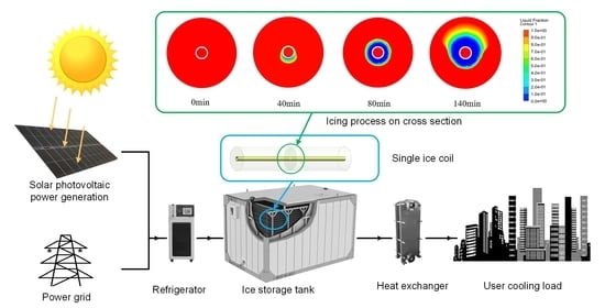
2.1. Model Description

The ice storage system described in this paper employs an aqueous solution of ethylene glycol as the refrigerant for facilitating heat transfer to the water inside the tube. A transient model of a single tube ice storage unit has been established, as depicted in Figure 1. During the simulation process, the heat transfer characteristics and water phase change process were analyzed in order to investigate the heat transfer coefficient, ice storage rate, and water temperature change patterns in the ice storage system. Table 1 shows the relevant calculation parameters used in the numerical analysis.
This paper presents numerical simulations of ice storage cells under three-dimensional unsteady conditions. The k-ε turbulence model and SIMPLE algorithm are utilized to simulate the icing process in water. The solidification/melting model and energy model are used in the simulation. The density reversal of water at 4.0 °C was taken into account in the simulation and it was represented through piecewise-linear assumptions. The velocity inlet and free outlet boundary conditions were applied. The heat exchanger tube boundary was set as the fluid–solid coupling interface, while the external interface was the third type of boundary condition, allowing for heat exchange with the external air through the adjustment of heat flux on the outer wall surface. The convergence criterion is a residual value below 10−5.
Structured grid partitioning of the model was utilized through ICEM and O-shaped segmentation of the middle HTF region. By adjusting the grid size, three different grid quantities of 215,461, 1,062,413, and 504,561 were selected for trial calculation with a time step of 0.5 s. The relative errors of the three grids were all less than 0.5%. Subsequently, a model with a total of 504,561 was used to select three time steps: 0.2 s, 0.5 s, and 1 s for trial calculation. The calculation results showed that the maximum relative error was less than 1.2%. Among them, the difference between 1 s and the other two step sizes is relatively large, while the difference between 0.5 s and 0.2 s is relatively small. To reduce calculation time, a time step of 0.5 s was selected. The number of meshes was 504,561, and a time step of 0.5 s was used, as shown in Figure 2. Considerations are given to meshing and time steps during numerical simulations.
In actual engineering, the radius of the coil is 10.00–15.00 mm and the wall thickness is 2.00 mm. Therefore, this article follows the actual engineering and sets the coil radius in the numerical simulation and experiments to 13.30 mm. The dimensional parameters of ice storage used in this study correspond to the experimental setup. The heat exchanger tube has a radius of 13.30 mm with a wall thickness of 2.00 mm. To ensure a sufficient water area for the ice storage process, the length and inner radius of the ice storage were set at 600.00 mm and 50.00 mm, respectively. The inlet temperature of the refrigerant was −6.0 °C, and the flow rate was 0.5 m/s. The initial water temperature of the ice storage was adjusted to 10.0 °C. To maintain consistency between the simulation and experiment, the simulation process’s monitoring points were precisely located as measurement point 3 in the experiment. Also, the simulation process incorporates insulation with the same thickness as the experiment.

2.2. Physical Formulation

2.2.1. Model Assumptions

(1) The flow of heat transfer fluid is modeled by momentum and mass conservation equations in the laminar flow state, and both water and aqueous glycol solutions are considered as incompressible and viscous working fluids in the text; (2) the flow of melting and solidifying phase change material is assumed to be laminar, unsteady, and incompressible; (3) the thermophysical properties of HTF, coil material, ice, and water are kept constant in the working temperature range; (4) linear assumption is used for the density change of liquid phase change materials, and the density inversion of water at 4.0 °C is simulated by the linear assumption; (5) viscous dissipation and volume change during the solid–liquid phase change are neglected.
Due to the limitations of numerical simulation based on theoretical frameworks and assumptions, it is necessary to describe the parameter changes in the numerical simulation through some assumptions. The purpose of the model assumption is to simplify the calculation and try to match the experimental situation as much as possible. Furthermore, through the comparison of numerical simulation and experimental results, the temperature change trend in the text can be observed, and the consistency between the experiment and numerical simulation can be obtained.

2.2.2. Model Equation

This section may be divided by subheadings. It should provide a concise and precise description of the experimental results, their interpretation, and the experimental conclusions that can be drawn.
By considering the above assumptions, as shown by the extension of the enthalpy method model to solve complex boundary problems on multidimensional problems, the flow and control equations in the ice storage cell are as follows:
Continuity equation:
u x + v y = 0
Momentum equation:
ρ u t + ρ U u = p x + μ u + C 1 γ γ 3 + q u
ρ v t + ρ U v = p y + μ v + C 1 γ γ 3 + q v
Continuity equation in the tube:
U = 0
Momentum equation:
U t + U U = P + 2 U
Energy equation:
h t + U h = 1 ρ α h
Energy equation outside the tube:
ρ h t + ( ρ U h ) = k c h ρ γ L t ρ γ L U = 0
Kozeny–Carman equation [25]:
K = K 0 γ 3 1 γ 2
In this paper, the process of ice formation or freezing was simulated using the enthalpy–porosity method [19].
γ = 0   i f   T < T s T T s T l T s   i f   T s < T < T l 1   i f   T > T l

2.3. Boundary Conditions

The following initial and boundary conditions are considered in the solidification process:
Initial conditions: The temperature at the initial moment is 10.0 °C. Boundary conditions: At the inlet of the cooling heat transfer fluid, a Poiseuille velocity distribution is applied. This velocity corresponds to Re = 1000 based on the inner diameter of the HTF tube [26]. The initial temperature of the heat transfer fluid is −6.0 °C, and the outflow is set at the outlet. Conjugate heat transfer is considered at the solid–liquid interface and the solid–solid phase interface [27,28]. Since there is heat transfer between the ice storage unit and the surrounding environment during the experiment, the third type of boundary conditions [29] is set in the numerical simulation, and the thermal conductivity of the outer wall surface is set to 2.0 W/(m·K).

3. Experimental Tests

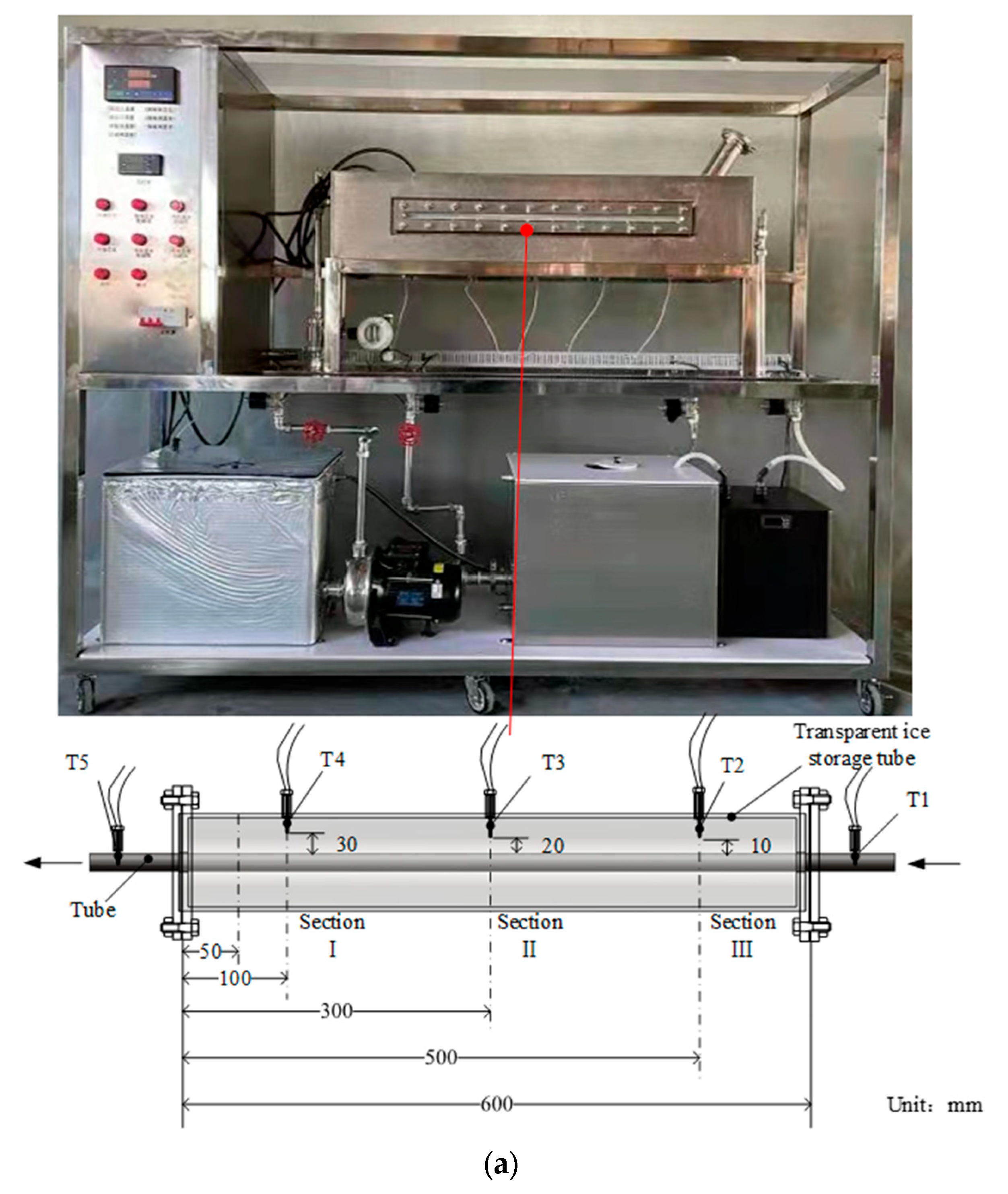
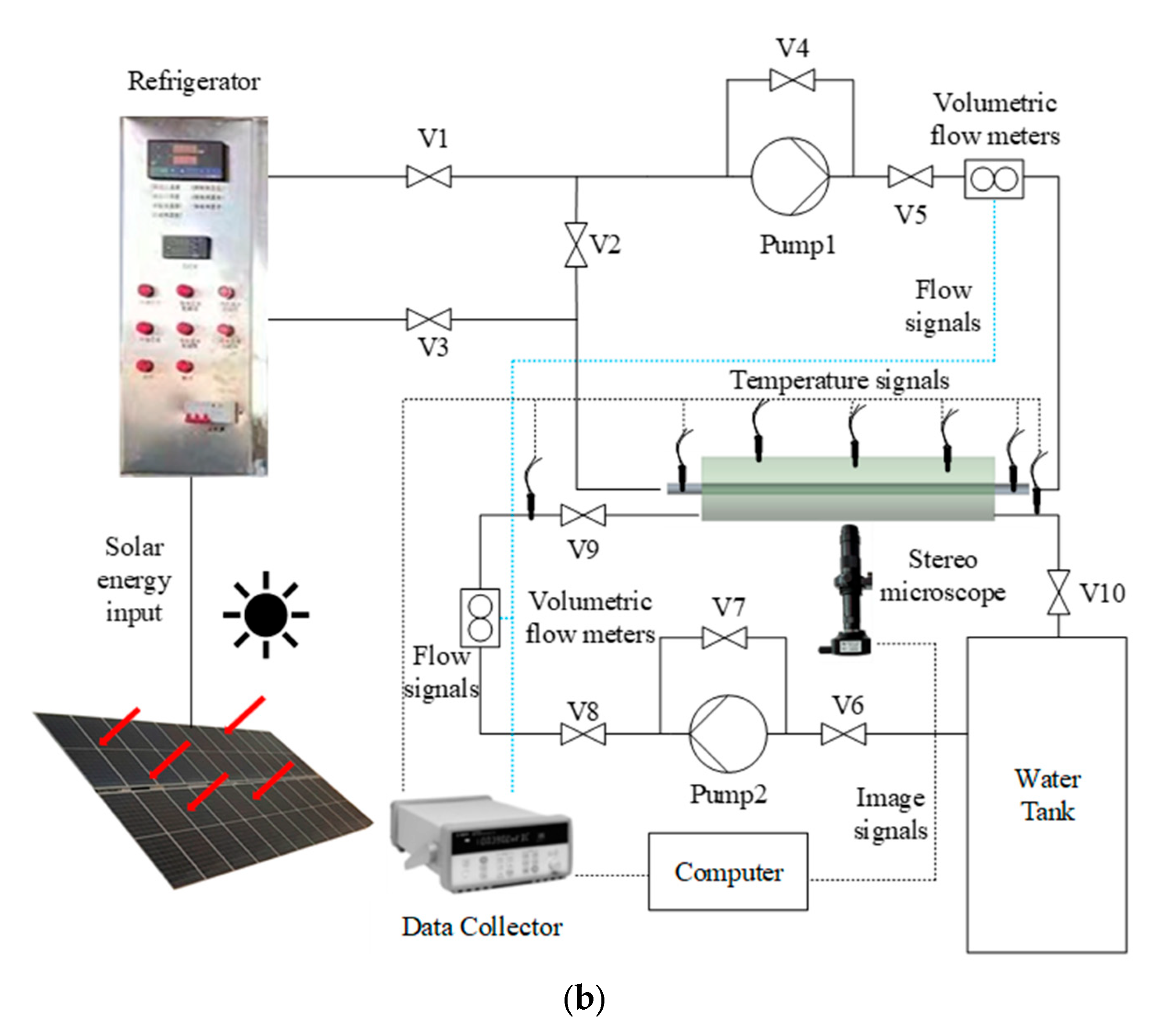
3.1. Experimental Setup

Figure 3 displays the experimental tube utilized in this study. For visualizing the ice alteration, a transparent ice storage unit tube was employed. The parameters of the experimental pipe section are depicted in the figure above. The length of the ice storage unit pipe measures 600.00 mm, and its outer diameter is 110.00 mm. The heat exchanger tube’s outer diameter is 26.60 mm, and it has a wall thickness of 2.00 mm. The variation in the internal ice layer was captured via a body microscope. As the natural convection of water can create an uneven temperature field inside the ice storage unit, temperature changes at various heights were monitored by placing thermocouples at different locations.

3.2. Experimental Operation Flow

The data acquisition module of the experiment consists of a volumetric flow meter, a T-type thermocouple, and a data collector, and the parameters of each instrument are shown in Table 1. The experiment started by turning on the thermostatic cooler, setting the circulating refrigeration temperature to −6.0 °C, and opening the internal circulation channel composed of V1, V2, and V3. Then, the flow rate of the refrigerant carrier of the volume flow meter is read, the body microscope is opened to monitor the ice storage of Section II, and at the same time, the data collector is used to monitor the temperature of the above five measurement points, with a monitoring time interval of 10 s. After the circulation temperature stabilizes to the set temperature, V4 and V5 are turned on, and V2 is turned off, so that the refrigerant carrier enters the external pipeline circulation for heat exchange with the water inside the ice storage unit.
Experimental initial conditions: The temperature at the initial moment is 10.0 °C, the same as the numerical simulation setting. Boundary conditions: At the inlet of the cooling heat transfer fluid, a Poiseuille velocity distribution is applied. This velocity corresponds to Re = 1000 based on the inner diameter of the HTF tube. The initial temperature of the heat transfer fluid is −6.0 °C. Conjugate heat transfer is considered at the solid–liquid interface and the solid–solid phase interface. Since there is heat transfer between the ice storage unit and the surrounding environment during the experiment, the third type of boundary conditions are set in the experimental.

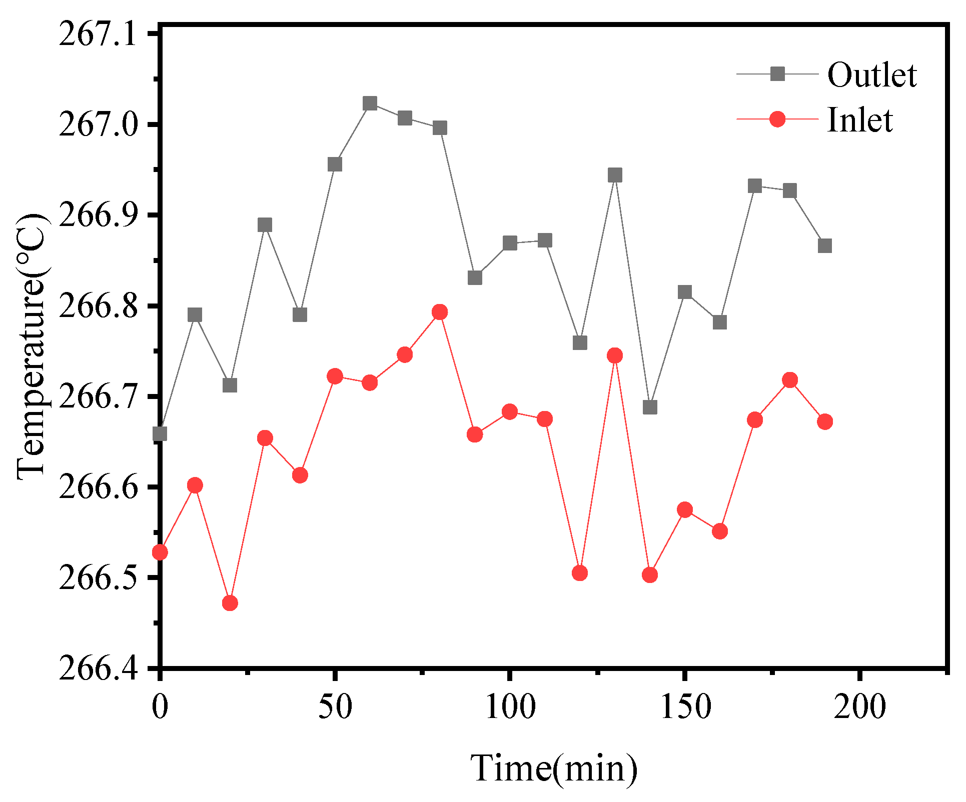
3.3. Experimental Error and Uncertainty

The T-type thermocouple temperature measurement range is −50.0 °C to 200.0 °C, and the measurement accuracy is ±0.5 °C. The accuracy of the sealed heating and cooling circulator is ±0.5 °C, the measurement accuracy of the volume flow meter is ±1%, and there is loss along the flow of the refrigerant carrier in the tube, so the flow rate decreases as it passes through the ice storage unit for heat exchange.

4. Results and Discussion

4.1. Mechanistic Analysis of the Icing Processes

This paper presents an analysis of the thickness of the horizontal ice layer in an experiment. The phase change began with the bottom of the coil freezing after 20 min, while the top gradually froze only after the ice layer at the bottom reached 3.21 mm. During the middle stage of the phase change, the water at the top of the heat exchanger tube underwent phase change after 40 min, and the growth rate of the ice layer at the top was higher than that at the bottom. The ice thickness at the top exceeded that at the bottom at 105 min, reaching 8.56 mm. In the late stage of the phase change, the thickness of the ice layer at the top was found to be 3.95 mm thicker than that at the bottom.
This paper presents an analysis of the horizontal ice layer thickness in an experiment. The phase change began with the lower coil freezing after 20 min, while the upper coil gradually froze only after the ice layer at the lower coil reached 3.21 mm. During the middle stage of the phase change, the water at the upper end of the heat exchanger tube underwent phase change after 40 min, and the ice layer growth rate at the top was higher than that at the bottom. The thickness of the ice layer at the top exceeded that at the bottom at 105 min, reaching 8.56 mm. In the later stage of the phase change, the ice layer at the top was found to be 3.95 mm thicker than that at the bottom, with the temperature of the water at the top lower than that at the bottom.
The results of ice formation in this experiment were compared and analyzed with the numerical simulation results to validate the study through mutual verification. Figure 4b presents the temperature variation at measurement point T3 in Figure 3a for both experimental and numerical simulations.
The experimentally obtained temperature data were slightly higher than the simulation temperature data due to instrument measurement errors and the impact of heat dissipation from the air and heat exchanger tube outside the ice storage unit during the experiment. Thus, the two temperatures differed slightly [26]. The maximum temperature difference between the experiment and the numerical simulation was 1.72 °C, with a maximum error of 0.63%, while the average temperature difference was 1.23 °C, with an average error of 0.45%. Given the long icing time in the latter part of the experiment, only some simulation results were selected to verify them against the experimental data. Comparing the experimental and numerical simulation results in Figure 4b, it can be concluded that the temperature change trend in the selected measurement point 3 of the ice storage unit is consistent between the experiment and numerical simulation. Therefore, the conclusions drawn from this experiment and numerical simulation can be deemed relatively reliable.
Table 2 highlights the alterations in the physical characteristics of ice and water within the range of −6.0 to 10.0 °C. Figure 4a depicts a graph of the density of water as per temperature. The density increases for temperatures 4.0 °C and above as the temperature goes down; during the cooling process from 0.0 to 4.0 °C, water density decreases; the gradient of density in the phase change at 0.0 °C observes a significant shift; and ice density falls to 917.00 kg/m3.

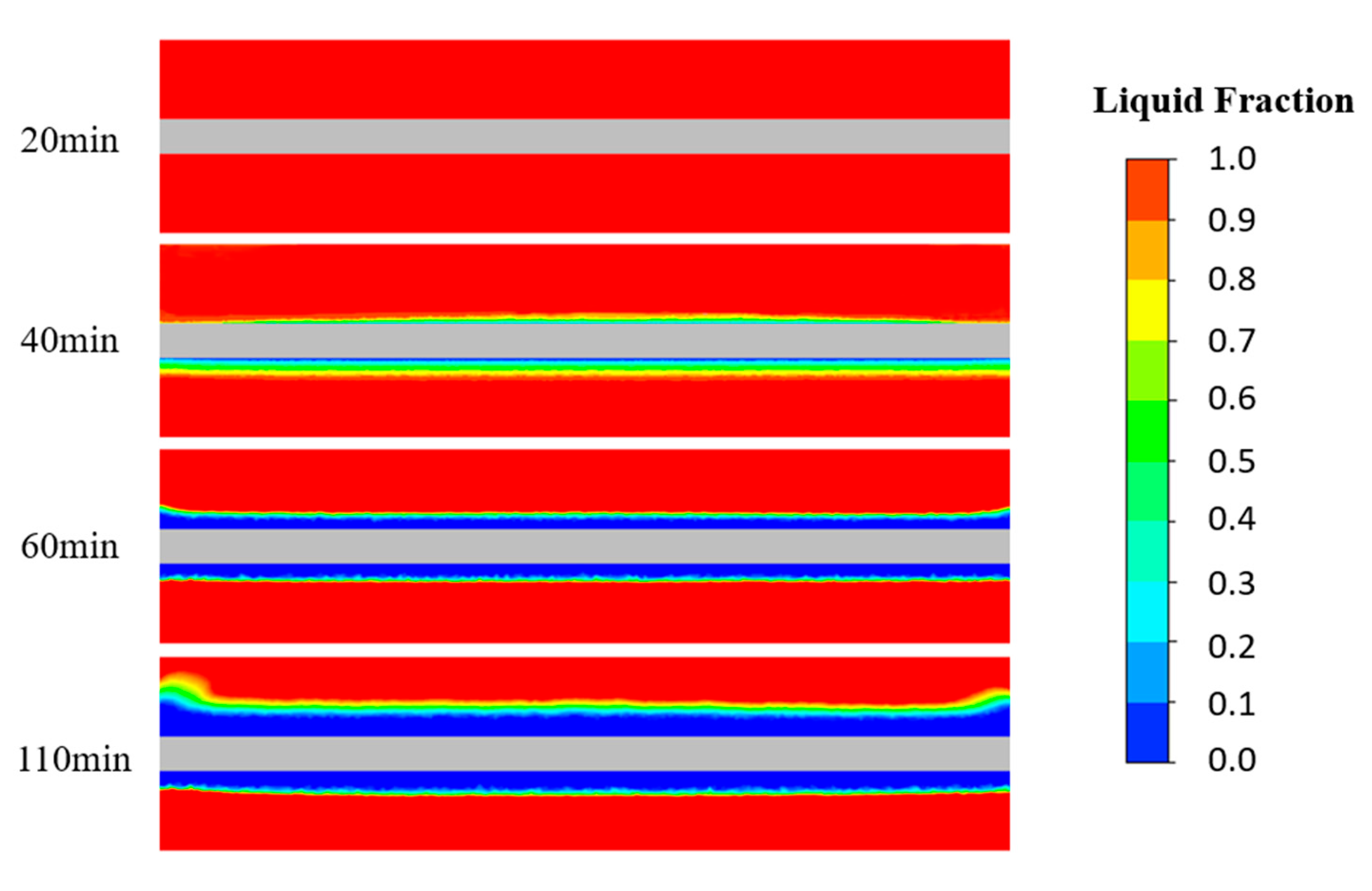
4.2. Liquid Phase Rate Cloud Analysis of the Ice Storage Process

The time-dependent growth of cross section II ice during the solidification process of the ice storage unit is presented in Figure 5. The solid phase is represented by the blue region, whereas the other regions depict the liquid phase. The red area at the center corresponds to the HTF, which appears in red in the liquid phase rate diagram since it does not undergo any phase change. Given that this study deals with the density inversion and natural convection of water during the cooling process, the simulation results are more in line with the physical reality.
Observations of the cloud diagram indicate that the ice sheet formed is not symmetrical around its axis. Therefore, it can be concluded that as well as heat conduction, other heat transfer mechanisms such as gravity and natural convection play a significant role during the phase change of water, resulting in an asymmetrical ice layer. It can also be seen from Figure 5 and Figure 6 that the ice layer formed at the bottom of the initial coil is more prominent than at the top due to the density reversal of water at lower temperatures (0.0 < T < 4.0 °C) [22]. This study analyzes the thickness of the ice layer for horizontally placed coils. During the early phase transition, the lower surface of the coil began to freeze at 20 min, forming a 2.50 mm ice layer, with the upper surface gradually starting to freeze. In the intermediate phase transition, the water on the upper surface of the heat exchanger tube began to phase transition at 40 min, and the growth rate of the ice layer on the upper surface was higher than that on the lower surface. The thickness of the ice layer on the upper surface was 8.56 mm at 105 min, gradually exceeding that on the lower surface. In the later stage of the phase transition, the ice layer formed on the upper surface was 3.86 mm thicker than that on the lower surface, and the water at the top of the ice storage unit had a lower temperature than that at the bottom.
As shown in Figure 7, the inlet of the ice storage unit experiences a lower temperature of the HTF compared to the outlet, resulting in the maximum ice thickness at the inlet. The average temperature difference between the inlet and outlet is 0.2 K. This temperature difference arises because the HTF passes through the heat exchanger tube with the water in the ice storage unit, causing a drop in the water temperature while increasing the HTF temperature. The HTF is cooled down via a thermostatic water bath and subsequently passes through the tube for further cooling. After the heat exchange process, the HTF returns to the thermostatic water bath to cool to a specified temperature.
In this study, the initial water temperature was set to 10.0 °C. As depicted in Figure 4a, water experiences a density reversal at 4.0 °C. The density increases as the temperature decreases from 10.0 °C to 4.0 °C, but decreases as the temperature goes below 4.0 °C. Thus, when the ice storage unit is horizontally placed, gravity causes a density stratification during the cooling process. Consequently, uneven icing occurs on the tube wall during the phase change process. During the cooling process from 10.0 °C to 4.0 °C, the refrigerant carrier’s initial temperature in the coil is −6.0 °C, resulting in a larger temperature gradient. This leads to a more noticeable natural convection in the pre-exchange period, creating two vortex regions on the heat exchanger tube’s left and right sides, with faster mixing of hot and cold fluids. Despite the density change, the low-temperature water at the bottom exchanges heat with the high-temperature water at the top using natural convection. However, the density reversal during the cooling process from 4.0 °C to below 0.0 °C significantly affects the icing process. Additionally, uneven icing between the top and bottom of the tube occurs during the cooling process from 4.0 °C to below 0.0 °C. Therefore, this paper aims to analyze the cooling process below 0.0 °C from 4.0 °C, while the cooling process from 10.0 °C to 4.0 °C will not be discussed.

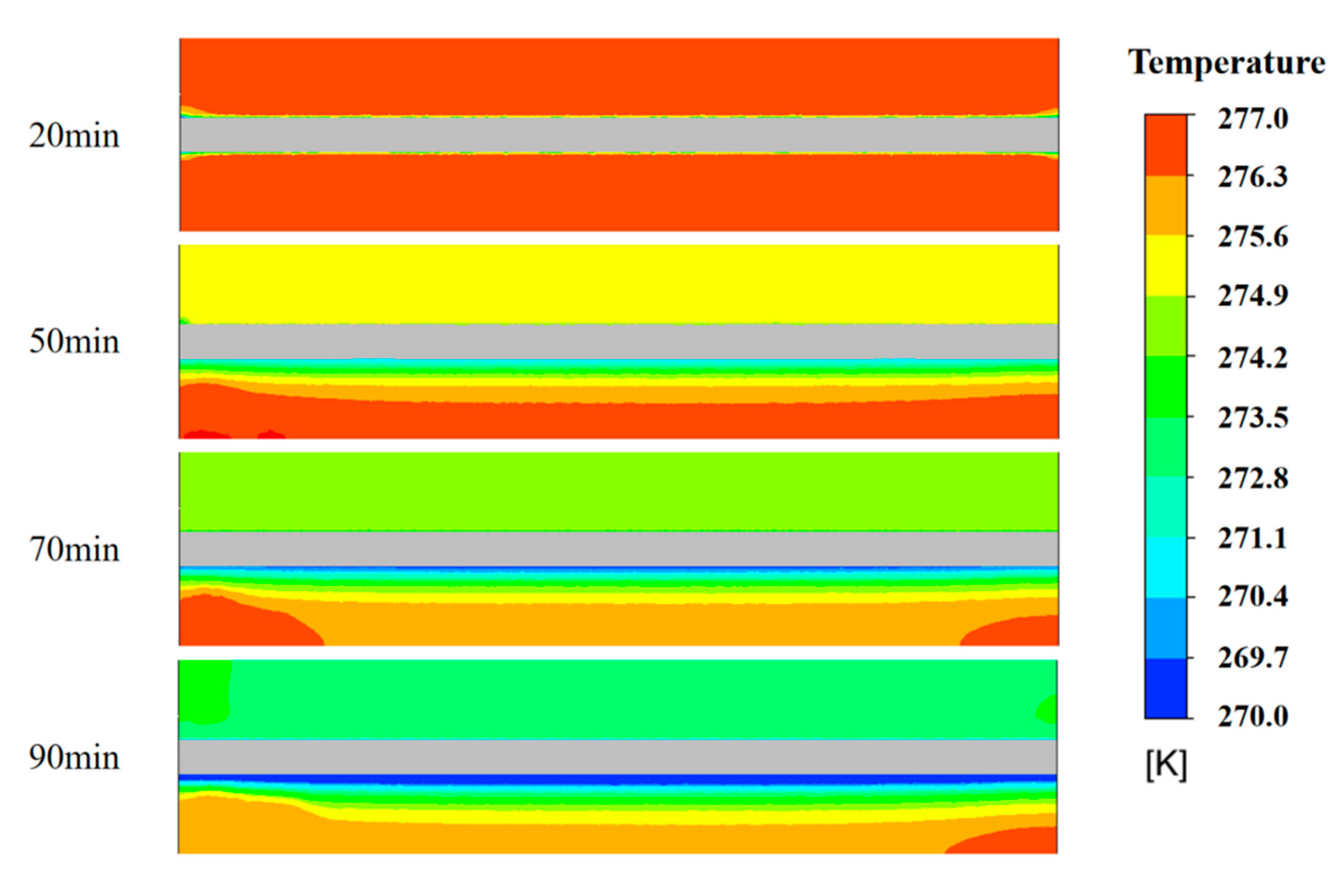
4.3. Temperature Cloud Analysis of the Ice Storage Process

Figure 8 depicts a temperature distribution cloud appearing in the central segment. The solidification process displays a substantial temperature gradient, thereby resulting in the intensification of natural convection. Moreover, noticeable density reversal is observable in all phases of the ice water transition from 10.0 °C to 4.0 °C, 4.0 °C to 0.0 °C, and 0.0 °C.
During the initial stage of water cooling, from 10.0 °C to 4.0 °C, the density of water increases as the temperature decreases. As a result, lower temperature water accumulates at the bottom while the higher temperature water collects at the top. The bottom layer contains 4.0 °C water, which, after further heat exchange, experiences a temperature drop beyond 4.0 °C. This causes the density to decrease and the lower temperature water to rise and mix with the higher temperature water. The curve representing the density of water between 0.0–10.0 °C resembles a parabola, with 4.0 °C representing the top. Consequently, when high-temperature and low-temperature water mixes, the top layer quickly reduces to roughly 4.0 °C. Thus, the study concludes that at some point, the water uniformly reduces to a temperature of 4.0 °C.
In the second stage, illustrated in Figure 8, water density decreases as temperature drops from 4.0 °C to 0.0 °C and the heat exchange tube and water continue to exchange heat. By comparing and examining the velocity vector diagram of the water with the tube cross section, it was observed that the colder water flows above the warmer water through the tube’s lower surface. As the low-temperature water passes through the lower surface by convection, it reaches the freezing point, resulting in the formation of ice nuclei and ice crystals on the lower surface around 0.0 °C. The thickness of the ice layer gradually increases, causing the thermal resistance of the lower surface to rise. Simultaneously, the upper surface experiences faster ice nuclei and crystal formation due to lower thermal resistance and colder water temperature. As a result, the ice growth rate increases. The lower density of low-temperature water moves to the upper part of the water, lowering the average temperature of the upper water surface below that of the bottom. Consequently, when ice begins to form on the upper surface, its growth rate is faster, gradually exceeding that of the lower surface.

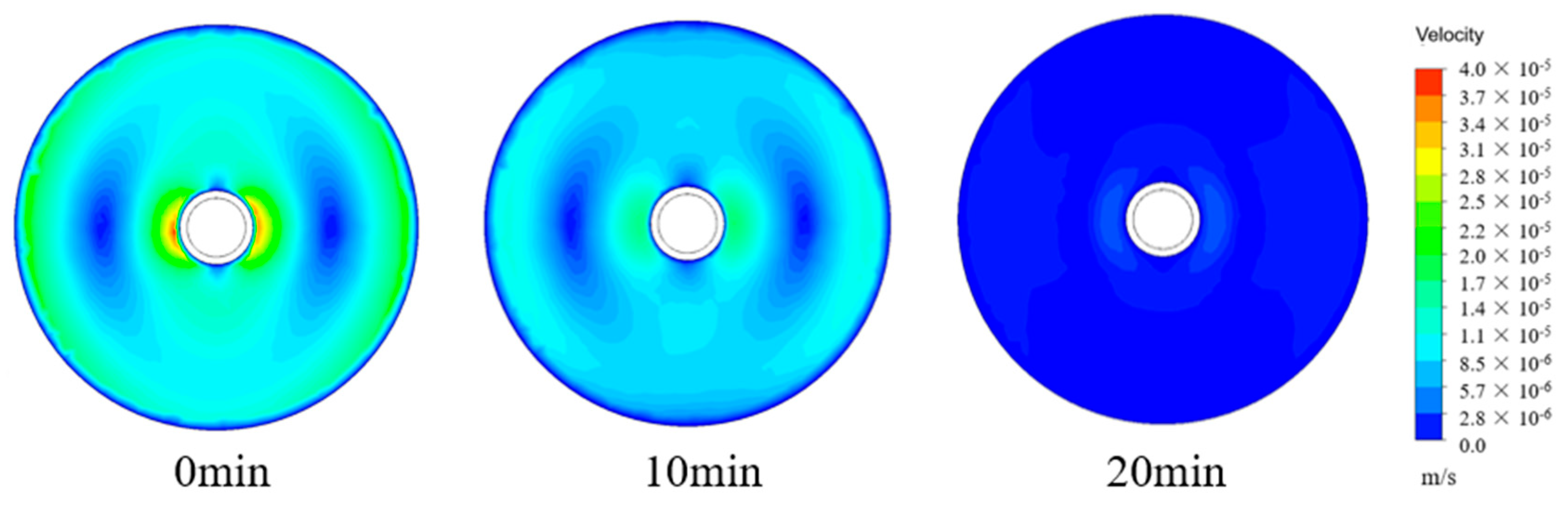
4.4. Velocity Cloud Analysis of the Ice Storage Process

Figure 9 shows a cross section of the velocity cloud during solidification, including the initial ice storage phase. The velocity field appears to have homogeneous distribution, with a decrease in flow field at the top during the pre-phase transition as water density increases due to the decrease in temperature. The diagram indicates that natural convection is more significant in the pre-ice storage phase, as the liquid phase region in the water is larger during this period.
With time, the velocity of the flow field in the cooling unit decreases, and two large vortex regions on the left and right are replaced with two smaller ones near the tube wall. The temperature of the water in the ice storage unit cools down to 4.0 °C and reaches a relatively equal state, causing a drop in natural convection within the unit. However, two smaller vortex regions on both sides of the tube wall persist due to the presence of low-temperature water around the tube.
The variation in velocity during the first stage of the second phase of water cooling is illustrated in Figure 10. In the cloud displaying velocity in a single tube, there are two symmetrical vortices that are apparent at the start of solidification. Natural convection velocity subsides at the commencement of solidification while the fluid moves upwards due to the alteration in water density with temperature within the temperature range of 4.0 °C down to 0.0 °C. At this point, the bottom of the flow has deposited water at a higher density of 4.0 °C, and the upper region’s return flow lacks the necessary momentum to enter the bottom resulting in its reflux back to the upper zone. The reflux water disrupts the big vortex area and breaks it up into two small vortices. Over time, each single vortex is separated into four above and two below forming six vortex areas in total. During the cooling period from 4.0 °C to 0.0 °C, the velocity of the flow field beneath reduces, and the vortex region above is more apparent. This results in the water on the surface below the coil quickly turning into an ice layer of a certain thickness. As seen in Figure 10, the temperature of the water in the whole zone remains low while low-temperature water enters the upper region due to its low density, leading to a gradual reduction in mixing and consequently reducing the velocity of the vortex region with time.
During ice storage, the formation of ice on the lower surface may cause a reduction in the free flow path between the bottom and the top, which could then result in a reduced vortex region in the upper part. At temperatures below 4.0 °C, the density of water may decrease and the higher temperature water may settle at the bottom of the water, thus leading to enhanced natural convection at the bottom. Meanwhile, lower temperature water may migrate to the top, resulting in weakened natural convection at the top. In the later stages of the icing process, the ice thickness on the lower surface may be lower than that on the upper surface, causing the water space at the bottom to be larger and therefore, leading to stronger natural convection at the bottom. Based on the cloud diagram, even though natural convection has a weak velocity field, it still plays a significant role in the ice formation pattern.
The diagrams of velocity clouds and liquid phase rates are compared and analyzed. During the pre-ice storage period, the water goes through a sensible thermal cooling phase, lowering from 10.0 °C to 4.0 °C. As a result, natural convection occurs only at the top and bottom due to density, with significant vortex areas observed on both sides of the diagram. These vortex areas are symmetric. In the middle stage of ice storage, natural convection at the top intensifies, while the convection at the bottom weakens. Consequently, the formation of ice on the lower surface begins faster. As the water reverses density, changing from 0.0 °C to 4.0 °C, the top vortex region becomes smaller, and the bottom vortex region increases. The ice formation on the upper surface of the heat exchanger tube grows faster, eventually exceeding the thickness of the ice on the lower surface.
As the ice storage process progresses in the ice storage tank, the thickness of the upper ice layer is greater than that of the lower part. Ice bridges are prone to appear between the upper and lower surfaces of the coil in the ice storage tank, causing a certain degree of impact during the ice melting process. In practical engineering, by adding stirring or air-blowing devices, the water temperature inside the unit is uniform, so that the surface of the coil can freeze evenly.
It is important to observe the icing process of a single coil, optimize its local structure, analyze the micro icing mechanism, and weaken the influence of natural convection and water density inversion on the ice storage process by adding devices. Studying the causes of uneven phenomena in the upper and lower ice layers can provide reference solutions for the arrangement design, spacing design, and ice melting time of ice storage coils.
The ice storage unit is a key component of the ice storage air conditioning system. Through the study of the icing characteristics of the ice storage unit, its ice storage characteristics and laws are summarized to weaken the influence of temperature stratification on the ice storage process and improve the ice storage efficiency. The improvement and development of ice storage air conditioning systems are of great significance.

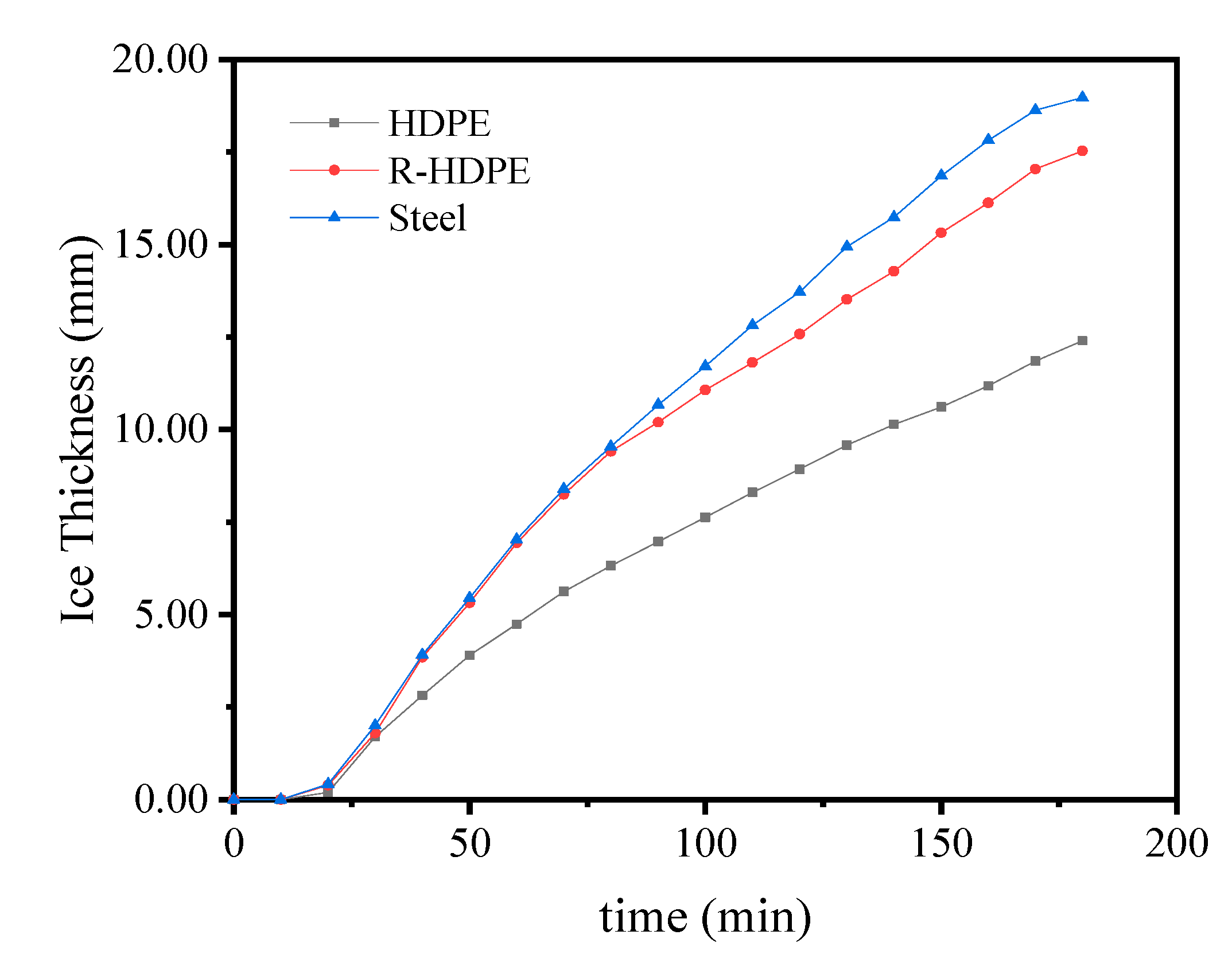
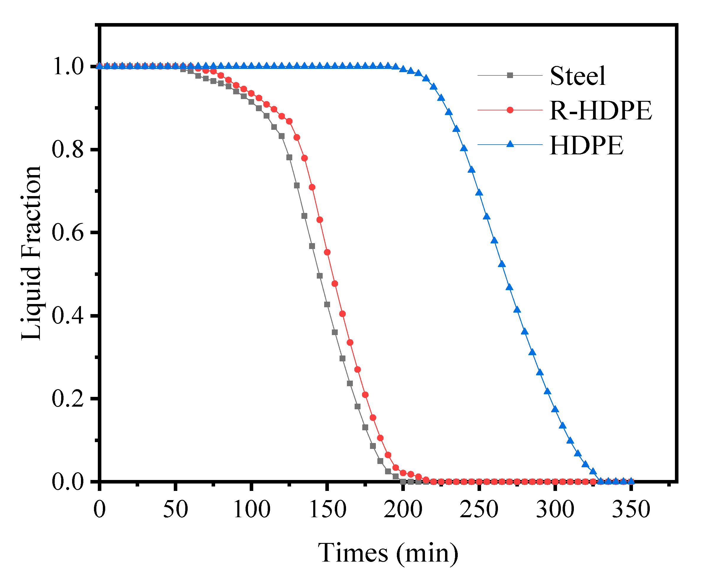
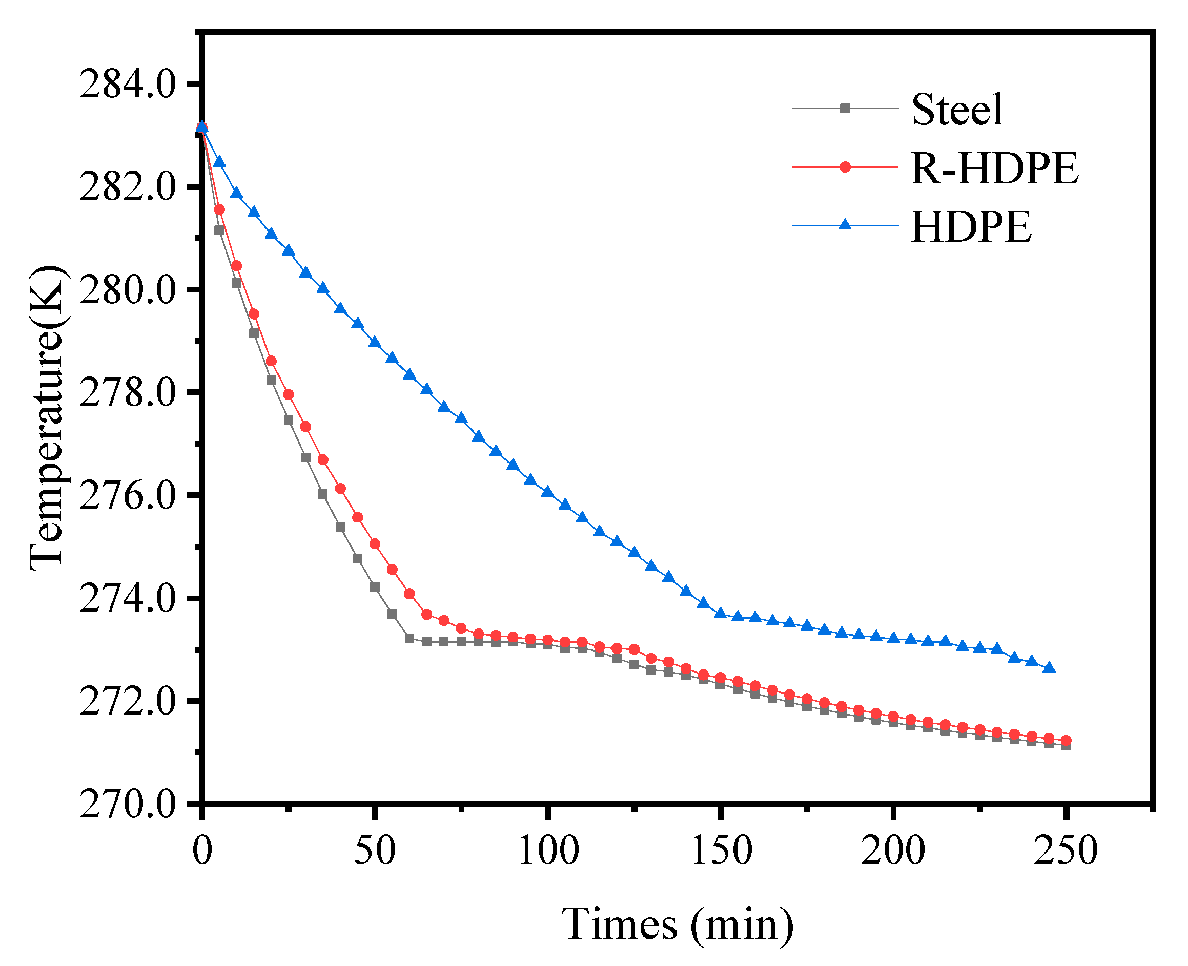
4.5. Effect of Thermal Conductivity of Ice Storage Process Tube

In this study, only changes in ice thickness over time were recorded to compare ice storage rates among pipes due to various external disturbances during the experiment. In numerical simulations, the ice storage process is analyzed under near-ideal conditions in which the liquid water phase rate is negligible. The freezing time required for complete ice formation in the storage tank is compared to analyze the ice storage rate among different pipes.
In Figure 11, the ice thickness of the different pipes was recorded during the experiment. The ice thickness of the steel pipe and R-HDPE (reinforced high-density polyethylene is a material made of high-density polyethylene after thermal conductivity enhancement treatment) pipe were close to each other, while the ice thickness of the HDPE pipe increased at a slower rate than the other two pipes. At 150 min, the ice thickness of both steel and R-HDPE reached 15.00 mm, while HDPE was only 10 mm. Due to the long icing process, only the ice thickness at 180 min was recorded in the experiment. At 180 min, the ice thicknesses of steel, R-HDPE, and HDPE were 18.97 mm, 17.53 mm, and 12.4 mm, respectively. The ice thickness of the R-HDPE pipe increased by 5.13 mm compared to the HDPE pipe at 180 min, while the ice thickness of the steel pipe was only 1.44 mm thicker than that of the R-HDPE pipe.
In this study, we performed a comparative analysis of the effects of three specific materials—steel pipe, HDPE pipe, and R-HDPE pipe—on the rate of ice storage. Figure 12 illustrates a comparison of the liquid phase rates of the three pipes during the ice storage process. The figure reveals that during the water sensible cooling stage, the liquid phase rate of all three pipes appears to follow the same trend, albeit with the HDPE pipe experiencing a longer sensible cooling stage. As we enter the isothermal phase change stage, we begin to observe the gradual emergence of differences in the liquid phase rate of the three pipes, with the carbon steel pipe and R-HDPE pipe exhibiting a more significant decrease in liquid phase rate than the HDPE pipe. Furthermore, the carbon steel pipe displays a slightly faster rate of decline than the R-HDPE pipe. Ultimately, towards the end of the ice storage process, the liquid phase rate of all three pipes decreases due to the water limitation and thermal resistance of the ice layer.
Figure 12 and Figure 13 display the complete freezing times of steel piping, R-HDPE piping, and HDPE piping at 195 min, 215 min, and 330 min, respectively. The ice accumulation rate of steel pipes is only 9.30% higher than that of R-HDPE pipes, and the R-HDPE’s rate is 34.85% higher than that of HDPE pipes. The liquid phase rate change curves of steel and R-HDPE piping, specifically the ice storage rates, are similar. However, there is a significant difference between the thermal conductivities of steel piping, which is 40.0 W/(m·K), and R-HDPE piping, which is only 2.8 W/(m·K).
The primary impediment to heat transfer from the ice layer is the thermal resistance of water and ice. With the thermal conductivity of ice being 2.2 W/(m·K) and water being 0.6 W/(m·K), it explains why there was a long cooling period for water in the initial stage because of the slow heat transfer rate due to water’s low conductivity [29]. During the middle stage of the cooling process, the ice layer became the primary hindrance to heat transfer because both carbon steel piping and R-HDPE piping had higher thermal conductivity when we compared them to both water and ice’s conductivity—which HDPE piping did not have. Thus, the ice storage rate of HDPE piping was lower than that of the other two pipes in the two stages of sensible thermal cooling and isothermal phase change.
As the numerical simulation area is smaller than in real engineering scenarios, the rate of change in the liquid phase is faster during the simulation process [30]. However, in an actual project, the presence of liquid water in the ice storage tank has a significant impact on the freezing process outside the coil, resulting in an increased time required for freezing.

5. Conclusions

Since the initial temperature of the water in the experiment and simulation was set to 10.0 °C, the phase change of the water is divided into two stages, 10.0 °C to 4.0 °C and 4.0 °C to below 0.0 °C, to refine the microscopic flow field and to investigate the ice storage process for coils with different thermal conductivities. The temperature and liquid phase rate fields of typical cross sections during the cooling process were analyzed, and the experimentally observed phenomena were analyzed using numerical simulations, leading to the following conclusions:
(1) The thermal conductivity of the coil material has a significant effect on the icing process. In particular, when the thermal conductivity of the pipe is lower than the thermal conductivity of ice and water, the lower the thermal conductivity, the longer the time required for icing.
(2) When the thermal conductivity of the coil material is higher than that of the ice, the increase in the thermal conductivity of the coil material has little effect on the time required for icing. The thermal conductivity of R-HDPE is only 2.8 W/(m·K), but the time required for complete freezing of the water outside the coil is reduced by 34.85%, and the thermal conductivity of carbon steel pipe is 40.0 W/(m·K), but the time required for complete freezing of the ice outside the coil is reduced by only 9.30%. R-HDPE is expected to replace carbon steel pipes in practical ice storage projects.
(3) The natural convection of water has an effect on the ice formation situation. The ice layer first appears on the lower outside surface of the coil, and an ice layer with a thickness of 2.50 mm is formed at this time. Over time, the ice layer on the top surface of the coil grows at a higher rate than the bottom surface. At 105 min, the ice thickness at the top exceeds that on the bottom, and finally, the ice thickness on the top surface of the coil was 3.85 mm thicker than that at the bottom surface.
(4) The natural convection in the ice storage is quite weak, and the maximum flow field velocity is 4 × 10⁻⁵ m/s during the whole cooling process, but it plays a crucial role in the icing process.

Author Contributions

Conceptualization, X.X. and C.C.; methodology, X.X.; software, X.X.; validation, X.X., C.C. and M.Z.; formal analysis, X.G.; investigation, C.C.; resources, X.X.; data curation, X.X.; writing—original draft preparation, X.X.; writing—review and editing, C.C.; visualization, X.X.; supervision, C.C.; project administration, C.C.; funding acquisition, C.C. All authors have read and agreed to the published version of the manuscript.

Funding

This work was supported by “Inner Mongolia-CAS” Science and technology cooperation project of Inner Mongolia Science and Technology Department (2020CG0066), focused on “Key technologies for solar energy application in ecological restoration and modern agriculture in deserts and saline-alkali lands”.

Data Availability Statement

Not applicable.

Conflicts of Interest

The authors declare no conflict of interest.

Nomenclature

Symbol uxdirection velocity-vector component [m/s]
Cporosity constant [C = 1.6 × 10³]vydirection velocity-vector component [m/s]
Hmlatent heat [J/kg]x,y,zcoordinate axes
hsensible enthalpy [J/kg]Greek symbols
K0empirical constant in K–Carman equationαthermal diffusivity [m2/s]
Kpermeabilityμviscosity [Pa·s]
kthermal conductivity [W/(m·K)]ρdensity [kg/m3]
Llength [mm]γliquid fraction
Ppressure [Pa]δthickness [mm]
qpermeability [10−3]Abbreviation
rradius [mm]CFDcomputational fluid dynamics
ttimes [s]HDPEhigh-density polyethylene
Ttemperature [K]HTFheat transfer fluid
Tsfreezing temperature [K]PCMphase change material
Uvelocity [m/s]

Appendix A

Table A1. Table of physical properties of water.
ItemsT [°C]ρ [kg/m3]cp [kJ/(kg·K)]λ [W/(m·K)]μ [Pa·s]h [kJ/kg]
ice−6.0~0.0917/2.2000000/335
water1.0999.8984.21760.55810800.00176335
2.0999.9404.21760.56058830.00176335
3.0999.9644.21760.56301620.00176335
4.0999.9724.21760.56539380.00176335
5.0999.9644.21760.56772330.00176335
6.0999.9404.21760.57000650.00176335
7.0999.9014.21760.57224530.00176335
8.0999.8484.21760.57444150.00176335
9.0999.7814.21760.57659650.00176335
10.0999.6994.21760.57871190.00176335

References

  1. Zeng, Y.; Zhang, R.W.; Wang, D.; Mu, Y.F.; Jia, H.J. A regional power grid operation and planning method considering renewable energy generation and load control. Appl. Energy 2019, 237, 304–313. [Google Scholar] [CrossRef]
  2. Chang, C.; Xu, X.Y.; Zheng, J.Y.; Dong, J.S.; Guo, X.X.; Zhao, M.Z. Research on Coil Type Ice Storage Air Conditioning Technology for Power Grid Peak Regulation. In Proceedings of the CSEE 2023 Congress Proceedings, Lisbon, Portugal, 29–31 March 2023; pp. 1–18. [Google Scholar]
  3. Sadi, M.; Arabkoohsar, A. Techno-economic analysis of off-grid solar-driven cold storage systems for preventing the waste of agricultural products in hot and humid climates. J. Clean. Prod. 2020, 275, 124143. [Google Scholar] [CrossRef]
  4. Chakravarty, K.H.; Sadi, M.; Chakravarty, H. A review on integration of renewable energy processes in vapor absorption chiller for sustainable cooling. Sustain. Energy Technol. Assess. 2022, 50, 101822. [Google Scholar] [CrossRef]
  5. Song, X.; Zhu, T.; Liu, L.X.; Cao, Z.J. Study on optimal ice storage capacity of ice thermal storage system and its influence factors. Energy Convers. Manag. 2018, 164, 288–300. [Google Scholar] [CrossRef]
  6. Thiem, S.; Born, A.; Danov, V.; Vandersickel, A.; Schafer, J.; Hamacher, T. Automated identification of a complex storage model and hardware implementation of a model-predictive controller for a cooling system with ice storage. Appl. Therm. Eng. 2017, 121, 922–940. [Google Scholar] [CrossRef]
  7. Salt, H.H. Experimental Study of Water Solidification Phenomenon for Ice-on-Coil Thermal Energy Storage Application Utilizing Falling Film. Appl. Therm. Eng. 2018, 146, 135–145. [Google Scholar]
  8. Cui, B.; Cao, D.; Xiao, F.; Wang, S.W. Model-based optimal design of active cool thermal energy storage for maximal life-cycle cost saving from demand management in commercial buildings. Appl. Energy 2017, 201, 382–396. [Google Scholar] [CrossRef]
  9. Zhou, Z.; Liu, P.; Li, Z.; Ni, W.D. An engineering approach to the optimal design of distributed energy systems in China. Appl. Therm. Eng. 2013, 53, 387–396. [Google Scholar] [CrossRef]
  10. Mousavi, A.S.S.; Poncet, S.; Sedighi, K.; Aghajani, M.D. Numerical modeling of the melting process in a shell and coil tube ice storage system for air-conditioning application. Appl. Sci. 2019, 9, 26–27. [Google Scholar]
  11. Chen, H.J.; Wang, W.P.; Chen, S.L. Optimization of an ice-storage air conditioning system using dynamic programming method. Refrigeration 2005, 25, 461–472. [Google Scholar] [CrossRef]
  12. Lu, Y.H.; Wang, S.W.; Sun, Y.J.; Yan, C.C. Optimal scheduling of buildings with energy generation and thermal energy storage under dynamic electricity pricing using mixed-integer nonlinear programming. Appl. Energy 2015, 147, 49–58. [Google Scholar] [CrossRef]
  13. Morgan, S. Experimental analysis of optimal control of passive and active building thermal storage inventory. Diss. Theses-Grad Work. 2007, 3, 1429–1432. [Google Scholar]
  14. Candanedo, J.A.; Dehkordi, V.R.; Stylianou, M. Model-based predictive control of an ice storage device in a building cooling system. Appl. Energy 2013, 111, 1032–1045. [Google Scholar] [CrossRef]
  15. Antoine, G.; Julien, E.; Matthieu, G.; Stéphane, G. Predictive control of multizone heating ventilation and air-conditioning systems in non-residential buildings. Appl. Soft Comput. 2015, 37, 847–862. [Google Scholar]
  16. Wang, B.L.; Li, X.T.; Zhang, M.Y.; Yang, X.D. Experimental Investigation of Discharge Performance and Temperature Distribution of an External Melt Ice-on-Coil Ice Storage Tank. Hvac. R. Res. 2003, 9, 291–308. [Google Scholar] [CrossRef]
  17. Hamzeh, H.A.; Miansari, M. Numerical study of tube arrangement and fin effects on improving the ice formation in ice-on-coil thermal storage systems. Int. Commun. Heat Mass Transf. 2020, 113, 104520. [Google Scholar] [CrossRef]
  18. Huang, Y.P.; Sun, Q.; Yao, F.; Zhang, C.B. Performance optimization of a finned shell-and-tube ice storage unit. Appl. Therm. Eng. 2020, 167, 114788. [Google Scholar] [CrossRef]
  19. Hosseinzadeh, K.; Alizadeh, M.; Tavakoli, M.H.; Ganji, D.D. Investigation of phase change material solidification process in a LHTESS in the presence of fins with variable thickness and hybrid nanoparticles. Appl. Therm. Eng. 2019, 152, 706–717. [Google Scholar] [CrossRef]
  20. Tay, N.; Bruno, F.; Belusko, M. Comparison of pinned and finned tubes in a phase change thermal energy storage system using CFD. Appl. Energy 2013, 104, 79–86. [Google Scholar] [CrossRef]
  21. Li, H.Y.; Hu, C.Z.; He, Y.C.; Tang, D.W.; Wang, K.M. Influence of fin parameters on the melting behavior in a horizontal shell-and-tube latent heat storage unit with longitudinal fins. J. Energy Storage 2021, 34, 102230. [Google Scholar] [CrossRef]
  22. Zhou, L.; Wu, Z.G. Analysis of HTFs,PCMs and fins effects on the thermal performance of shell-tube thermal energy storage units. Sol. Energy 2015, 122, 382–395. [Google Scholar]
  23. Scanlon, T.J.; Stickland, M.T. An experimental and numerical investigation of natural convection melting. Int. Commun. Heat Mass Transf. 2001, 28, 181–190. [Google Scholar] [CrossRef]
  24. Dekhil, M.A.; Tala, J.V.S.; Bulliard-Sauret, O.; Bougeard, D. Numerical analysis of the performance enhancement of a latent heat storage shell and tube unit using finned tubes during melting and solidification. Appl. Therm. Eng. 2021, 192, 116866. [Google Scholar] [CrossRef]
  25. Voller, V.R.; Prakash, C. A fixed grid numerical modelling methodology for convection-diffusion mushy region phase-change problems. Int. J. Heat Mass Transf. 1987, 30, 1709–1719. [Google Scholar] [CrossRef]
  26. Jannesari, H.; Abdollahi, N. Experimental and numerical study of thin ring and annular fin effects on improving the ice formation in ice-on-coil thermal storage systems. Appl. Energy 2017, 189, 369–384. [Google Scholar] [CrossRef]
  27. Chen, J.S.; Chen, J.T.; Liu, C.W.; Liang, C.P.; Lin, C.W. Analytical solutions to two-dimensional advection–dispersion equation in cylindrical coordinates in finite domain subject to first-and third-type inlet boundary conditions. J. Hydrol. 2011, 405, 522–531. [Google Scholar] [CrossRef]
  28. Zhang, Y.; Yuan, G.F.; Wang, Y.; Gao, P.H.; Fan, C.G.; Wang, Z.F. Solidification of an annular finned tube ice storage unit. Appl. Therm. Eng. 2022, 212, 118567. [Google Scholar] [CrossRef]
  29. Sang, W.H.; Lee, Y.T.; Chung, J.D.; Kim, S.T.; Kim, T.; Lee, K.H. Efficient numerical approach for simulating a full-scale vertical ice-on-coil type latent thermal storage tank. Int. Commun. Heat Mass Transf. 2016, 78, 29–38. [Google Scholar] [CrossRef]
  30. Zheng, J.Y.; Chang, C.; Xu, X.Y.; Dong, J.S.; Zhao, M.Z.; Zhang, S.G. Effect of material characteristics on ice storage performance of an external melting ice-on-coil tube. Energy Proc. 2021, 24, 1–5. [Google Scholar]
Figure 1. Geometric model of the ice-on-coil tube.
Energies 16 05511 g001
Figure 2. Meshes for the simulation.
Energies 16 05511 g002
Figure 3. (a) Actual picture of the laboratory table and schematic diagram of the ice storage unit; (b) Schematic diagram of the ice storage unit system.
Energies 16 05511 g003aEnergies 16 05511 g003b
Figure 4. (a) Graph of the variation of water density with temperature (Appendix A); (b) Comparison of experimental and simulated temperatures.
Energies 16 05511 g004aEnergies 16 05511 g004b
Figure 5. Relevant images of the ice layer at different times.
Energies 16 05511 g005
Figure 6. Liquid fraction change during ice storage.
Energies 16 05511 g006
Figure 7. Variation of inlet and outlet temperature with time.
Energies 16 05511 g007
Figure 8. Diagram of water temperature change during ice storage.
Energies 16 05511 g008
Figure 9. Velocity cloud of the first stage of the ice storage process.
Energies 16 05511 g009
Figure 10. Velocity cloud of the second stage of the ice storage process.
Energies 16 05511 g010
Figure 11. Variation of ice thickness with time for different tubes.
Energies 16 05511 g011
Figure 12. Variation of liquid phase rate with time for different tubes.
Energies 16 05511 g012
Figure 13. Variation of average temperature with time for different tubes.
Energies 16 05511 g013
Table 1. Numerical model calculation parameters.
ItemsSymbolsUnitsValues
Length of the ice storage L(mm)600.0
Inner radius of the ice storage r3(mm)50.0
Outer radius of the coil r2(mm)13.3
Inner radius of the coilr1(mm)11.2
Initial temperature of ethylene glycol T1(°C)−6.0
Flow rate of ethylene glycol U(m/s)0.5
Initial water temperatureT2(°C)10.0
Thickness of insulation layer δ(mm)20.0
Table 2. Table of the physical parameters of different coil materials.
Itemsλ[W/(m·K)]Length [mm]Thickness [mm]
HDPE0.2600.002.00
R-HDPE2.8600.002.00
Steel40.0600.002.00
Disclaimer/Publisher’s Note: The statements, opinions and data contained in all publications are solely those of the individual author(s) and contributor(s) and not of MDPI and/or the editor(s). MDPI and/or the editor(s) disclaim responsibility for any injury to people or property resulting from any ideas, methods, instructions or products referred to in the content.

