Determination of Heat Transfer Correlations for Fluids Flowing through Plate Heat Exchangers Needed for Online Monitoring of District Heat Exchanger Fouling

Abstract

This article deals with the problem of estimating the degree of fouling of plate heat exchangers (PHEs) used in district heating substations (where the working medium is water). A method for calculating the thermal resistance of fouling is proposed based on a comparison of the thermal resistance of a fouled and clean heat exchanger. The thermal resistance of the heat exchanger for both fouled and clean apparatuses is determined as the inverse of their overall heat transfer coefficient. In the method, the heat transfer coefficients necessary to determine the overall heat transfer coefficient of the clean exchanger are calculated using a modified Wilson method. Moreover, the heat transfer coefficients on the clean heat exchanger plates’ cold water side are determined based on experimental tests. The computational algorithm presented in this paper will make it possible to develop software to monitor and thus optimise the operation of district heating substations.

1. Introduction

PHEs are used in many areas of industry. They are commonly used in heating; refrigeration; district heating; and various industries, such as the food processing, brewing, pharmaceuticals, oil, gas, and chemical industries. These heat exchangers are composed of a number of plates with a thickness of approximately 0.3 (Brazed PHE) or 0.4 mm (Plate-and-Frame PHE) [1]. Depending on the area of use, heat exchangers differ in the way the plates are connected (brazed, welded, gasketed, and semi-welded) and the material of the plates (stainless steel or more sophisticated alloys, e.g., alloy 254 SMO, alloy C-276, titanium, palladium-stabilised titanium, Incoloy, and Hastelloy) [1]. Their popularity is due to their small size, but, at the same time, high thermal efficiency. For example, compared with shell-and-tube heat exchangers, the total heat transfer coefficient of the PHE is about twice as high [2]. The large value of the overall heat transfer coefficient is caused by the embossing on the plates, due to which the fluid flowing between the plates is disturbed, increasing the intensity of heat transfer. The embossing on the plates also increases their stiffness, which allows PHEs to operate at high pressures. The high heat output of PHEs is due not only to the higher values of overall heat transfer coefficients, but also to the fact that the embossing on the plates increases the surface area of heat transfer of these apparatuses.

A significant problem in the operation of PHEs is the efficient assessment of the fouling condition of the apparatus. They should be subjected to regular cleaning; otherwise, fouling will cause a decrease in the heat output of the heat exchanger, as well as an increase in the pressure drop of fluid. Contaminants are deposited in heat exchangers regardless of the fluid physical state [3,4,5]. The literature indicates that in some industries (e.g., the dairy industry [5,6,7,8]), the occurrence of contaminants in this type of apparatus is a serious problem.

Although fouling in heat exchangers is a problem, as mentioned earlier, in the case of PHEs, due to disturbed fluid flow, there is partial self-cleaning of the apparatuses. This means that PHEs do not foul as quickly as, for example, shell-and-tube heat exchangers. In addition, the deposition of fouling can be reduced by using the appropriate shape of plate embossments or appropriate coatings [3,4,5,9,10] or by choosing the optimal fluid velocity [11,12].

The optimisation of the cleaning process for PHEs at district heating substations could be aided by either the capability to determine the rate at which the layer of deposits builds up on the plates or by monitoring the thermal resistance of the heat exchangers. One of the methods proposed in the literature is to predict the formation of a deposit layer using numerical models of PHEs [7,8,11]. All numerical models to predict the formation of deposits in PHEs, described in [7,8,11], also considered their partial washout by the flowing fluid. In [11], the authors have numerically analysed the formation of a layer of fouling in a plate heat exchanger using 3D Realisable κ-ε with non-equilibrium wall functions modelling and the von Karman analogy for three different apparatus (with different geometries) and taking into consideration the influence of geometry on fluid dynamics. The analyses were supported by experimental studies. The accuracy of the proposed solution is satisfactory, but its limitation is that the research can only be performed for turbulent flow. In addition, more complex models based on Computational Fluid Mechanics (CFD) tend to have long calculation times. Most articles investigating fouling in PHEs are related to the dairy industry, and articles [7,8] are examples of this. Both articles take a different approach to modelling the formation of the contamination layer from the previous one, based on the principle of conservation of mass and energy. In paper [7], a 2D dynamic model of a PHE is proposed, allowing simulation with arbitrary cold and hot fluid flow configurations and with different fouling and cleaning kinetics. On the other hand, the paper [8] discusses the problem of milk pasteurisation in a High-Temperature-Pasteurisation-Process plate pasteuriser. A model of the entire plant, including PHEs, was made. The study adopted a simple 1D model of the rate of fouling of the PHEs with protein with minimum calculation time and investigated the effect of the thickness of the resulting fouling layer on the milk pasteurisation temperature. Both approaches presented are not applicable to PHEs in district heating substations because of the different mechanisms of fouling formation due to the different types of working fluid.

Regardless of the increasing development of CFD models, the best and simplest method of evaluating contamination in PHEs is to determine their thermal resistance via experiments. An example of just such an approach is presented in [13]. The authors of this paper aimed to determine the thermal resistance of a plate heat exchanger included in a district heating substation. Like the method developed and presented in this paper, the technique described by S.B. Genica et al. in [13] compares the thermal resistance of a fouled and clean heat exchanger. However, in their study, based on the four plate heat exchanger models analysed, the thermal resistance of the fouling was determined as a function of shear stress. In addition, the overall heat transfer coefficient for a clean heat exchanger was determined based on its manufacturer’s design software. The need to use this software is a limitation of this method. A literature review indicates that there is still a need to develop a quick and simple method to optimise the PHEs cleaning process.

This paper proposes a method for determining the thermal resistance of fouled PHEs using experimental studies. It consists of determining the thermal resistance of a clean and a fouled heat exchanger. If the difference between these resistances exceeds a preset value, the heat exchanger will require cleaning. The thermal resistance of a fouled heat exchanger is determined by measurements from the transformed Peclet equation. At the same time, the thermal resistance of a clean heat exchanger is determined as the sum of the thermal resistances of heat transfer and heat conduction, where the thermal transfer resistances are counted from correlations on the Nusselt number of the cold and hot fluid. These, in turn, are calculated from the proposed modified iterative Wilson method. This paper presents the results of calculations using a new modification of the Wilson method on a constructed experimental test stand.

2. Method for Evaluating Fouling of the Heat Exchanger

In the method, the degree of fouling of the PHE will be estimated by comparing the thermal resistance of the fouled $R_{fouled}$ and clean $R_{clean}$ heat exchanger:

$$\Delta R=R_{fouled}-R_{clean}$$

(1)

The thermal resistance of a contaminated heat exchanger will be calculated as the reciprocal of the overall heat transfer coefficient $k_{fouled}$ determined using the measured data:

$$R_{fouled}=\frac{1}{k_{fouled}}$$

(2)

In the case of a clean heat exchanger, the thermal resistance will be determined using the following equation:

$$R_{clean}=\frac{1}{k_{clean}}=\frac{1}{{\alpha }_c}+\frac{{\delta }_p}{{\lambda }_p}+\frac{1}{{\alpha }_h}$$

(3)

where $k_{clean}$ is the overall heat transfer coefficient of a clean heat exchanger in W/(m²K); ${\alpha }_h$ and ${\alpha }_c$ are the heat transfer coefficients of the heat exchanger’s hot and cold sides in W/(m²K), respectively; ${\delta }_p$ is the thickness of the plate in m; and ${\lambda }_p$ is the thermal conductivity coefficient of the heat exchanger plate material in W/(mK). The heat transfer coefficients ${\alpha }_h$ and ${\alpha }_c$ will be calculated from the Nusselt numbers for hot fluid $N{u}_h$ and cold fluid $N{u}_c$, respectively. The new method for determining constants in the correlations per Nusselt number is described in Section 4.

Cleaning of the heat exchanger will be necessary when the following inequality is met:

$$\Delta R\ge R_{lim}$$

(4)

where $R_{lim}$ is the limit value of thermal resistance in (m²K)/W.

3. Determination of the Overall Heat Transfer Coefficient in the Heat Exchanger of a District Heating Substation

To determine the overall heat transfer coefficient $k$ of the heat exchanger, the formula obtained from the Peclet equation can be used [14]:

$$\dot{Q}=FkA\Delta T_m$$

(5)

where $\dot{Q}$ is the heat exchanger heat power in W, $F$ is the correction factor that depends on the heat exchanger type ($F$ = 1 for parallel-flow and counter-flow heat exchangers [15]), $k$ is overall heat transfer coefficient in W/(m²K), $A$ is the total heat transfer surface area in m², and $\Delta T_m$ is the logarithmic mean temperature difference in K.

The heat output of the heat exchanger can be calculated from the energy balance equation for the hot fluid flowing through the apparatus, as ${\dot{Q}}_h$, based on the known mass flow rate ${\dot{m}}_h$ and its average specific heat ${\overline{c}}_{wh}$, as well as the fluid temperatures at inlet $T_{h1}$ and outlet $T_{h2}$.

Similarly, the heat flow rate in the heat exchanger can be calculated from the energy balance equation for the cold fluid, as ${\dot{Q}}_c$, based on the known mass flow rate ${\dot{m}}_c$, average specific heat ${\overline{c}}_{wc}$, and temperatures of the cold fluid at the inlet $T_{c1}$ and outlet $T_{c2}$ of the apparatus.

If there is no heat loss from the heat exchanger to the surroundings, then ${\dot{Q}}_h={\dot{Q}}_c$. In practice, even though thermal insulation is used on the heat exchangers, heat losses occur and the heat flow rate value ${\dot{Q}}_h$ is higher than the value ${\dot{Q}}_c$. In this case, the average value of the heat flow rate ${\dot{Q}}_m$ that is transferred in the apparatus from hot to cold fluid can be calculated as [16]

$${\dot{Q}}_m=\frac{{\dot{Q}}_h+{\dot{Q}}_c}{2}$$

(6)

Based on the average heat flow rate ${\dot{Q}}_m$, the heat transfer surface area $A$ and the mean logarithmic temperature difference $\Delta T_m$, the overall heat transfer coefficient $k$ for the fouled heat exchangers can be obtained using the transformed Equation (5):

$$k=\frac{{\dot{Q}}_m}{FA\Delta T_m}$$

(7)

4. Determination of the Nusselt Number Correlation for Cold and Hot Fluid in a Clean Heat Exchanger

The method proposed in the article is experimental and modifies the popular Wilson graphical method. Thus, the laboratory studies to identify the cold fluid Nusselt number correlation are based on measuring cold and hot fluid parameters at a constant hot flow rate and for various cold fluid flow rate values. In turn, to determine the hot fluid’s Nusselt number correlation, laboratory testing in the heat exchanger must be carried out at a constant hot fluid flow rate and a variable flow rate of the hot fluid.

The developed method is based on iterative calculations. The single-iteration calculation algorithm presented in this chapter is for a single measurement point. Performing a series of iterations for several measurement points based on the described algorithm allows us to determine the Nusselt number correlation of the cold fluid $N{u}_c$.

At the beginning of the iteration, the Nusselt number $N{u}_c$ is calculated for the selected $N$ measurement points using a modified Colburn correlation [17]:

$$N{u}_c=C_{c1}R{e}_c^{0.8}P{r}_c^{0.33}+C_{c2}$$

(8)

in which the constant $C_{c1}$ replaces the value of 0.023 and an additional constant $C_{c2}$ is inserted. In Equation (8), $R{e}_c$ and $P{r}_c$ denote the Reynolds and the Prandtl numbers of the cold fluid, respectively.

Based on the calculated Nusselt number $N{u}_c$, the heat transfer coefficient at the surface washed by the cold fluid ${\alpha }_c$ is calculated using the following equation:

$${\alpha }_c=\frac{N{u}_c{\lambda }_c}{d_{hydr,c}}$$

(9)

where $d_{hydr,c}$ is the hydraulic diameter of the channel the cold fluid flows through in m and ${\lambda }_c$ is the cold fluid thermal conductivity coefficient in W/(mK).

Next, using the heat transfer coefficient on the cold side of the heat exchanger ${\alpha }_c$, the heat transfer coefficient on the surface washed by the hot fluid ${\alpha }_h^{\prime }$ is determined using the transformed Equation (3) for the overall thermal resistance of the PHE:

$$\frac{1}{{\alpha }_h^{\prime }}=\frac{1}{k}-\frac{1}{{\alpha }_c}-\frac{{\delta }_p}{{\lambda }_p}$$

(10)

Thereafter, based on the computed hot-side heat transfer coefficient ${\alpha }_h^{\prime }$, we can compute the hot fluid Nusselt number $N{u}_h^{\prime }$ using the following equation:

$$N{u}_h^{\prime }=\frac{{\alpha }_h^{\prime } d_{hydr,h}}{{\lambda }_h}$$

(11)

where $d_{hydr,h}$ is the hydraulic diameter of the channel the hot fluid flows through in m and ${\lambda }_h$ is the hot fluid thermal conductivity coefficient in W/(mK).

The calculated values of the Nusselt number $N{u}_h^{\prime }$ for $N$ measurement points allow for the determination of the constants $C_{h1}$ and $C_{h2}$ via approximation with a linear function of the following form:

$$N{u}_h=C_{h1}R{e}_h^{0.8}P{r}_h^{0.33}+C_{h2}$$

(12)

using the linear regression method.

In Equation (12), $R{e}_h$ and $P{r}_h$ are the Reynolds and the Prandtl numbers of hot fluid, respectively.

With the determined coefficients $C_{h1}$ and $C_{h2}$ (slope and vertical intercept of the function, respectively), the Nusselt number $N{u}_h$ is recalculated using Equation (12).

In the next step of the algorithm, the hot-side heat transfer coefficient ${\alpha }_h$ is computed:

$${\alpha }_h=\frac{N{u}_{h }{\lambda }_h}{d_{hydr,h}}$$

(13)

Based on the calculated heat transfer coefficient on the hot side of the heat exchanger ${\alpha }_h$, the cold-side heat transfer coefficient ${\alpha }_c^{\prime }$ can be calculated as follows:

$$\frac{1}{{\alpha }_c^{\prime }}=\frac{1}{k}-\frac{1}{{\alpha }_h}-\frac{{\delta }_p}{{\lambda }_p}$$

(14)

The Nusselt number of the cold fluid $N{u}_c^{\prime }$ is then determined as follows:

$$N{u}_c^{\prime }=\frac{{\alpha }_c^{\prime } d_{hydr,c}}{{\lambda }_c}$$

(15)

From the calculated Nusselt number $N{u}_c$ and the Prandtl $P{r}_c$ and Reynolds $R{e}_c$ numbers of the cold fluid at the end of the iterative loop, the constants $C_{c1}$ and $C_{c2}$ are determined for $N$ measurement points by approximating the data with a linear function (8) using the linear regression method.

The iterations are continued as long as the following conditions are met:

$$\left|\frac{C_{c1}^{\left(j\right)}-C_{c1}^{\left(j-1\right)}}{C_{c1}^{\left(j\right)}}\right|\le {\epsilon }_{c1}$$

(16)

and

$$\left|\frac{C_{c2}^{\left(j\right)}-C_{c2}^{\left(j-1\right)}}{C_{c2}^{\left(j\right)}}\right|\le {\epsilon }_{c2}$$

(17)

where j is the number of the iteration and ${\epsilon }_{c1}$ and ${\epsilon }_{c2}$ have small values (less than 0.001 for ${\epsilon }_{c1}$ and 0.01 for ${\epsilon }_{c2}$)$.$

The calculation algorithm for determining the constants $C_{h1}$ and $C_{h2}$ in the Nusselt number correlation for hot fluid can be written analogously to the algorithm for determining the constants $C_{c1}$ and $C_{c2}$ in the Nusselt number correlation for cold fluid presented above.

In the single-iteration loop, an apostrophe “ $\prime$ ” has been used in some symbols, i.e., in the heat transfer coefficient $\alpha$ and the Nusselt number $Nu$ for cold and hot fluid. This was performed as such because, in the single-iteration loop, these values appear and are calculated twice. The rule of thumb was adopted, with the symbol “ $\prime$ ” denoting the heat transfer coefficients calculated from the formula for the overall heat transfer resistance between the cold and hot fluid in the heat exchanger (Equations (10) and (14)) and the Nusselt numbers calculated from them (Equations (11) and (15)).

Plate heat exchangers in district heating substations may differ in design, i.e., in the number of plates or the type of corrugations. The proposed computational algorithm will allow the determination of constants in the correlations on the Nusselt numbers for cold and hot fluid flowing through a specific clean apparatus model. This, in turn, will make it possible to determine its total thermal resistance for any operation conditions.

5. Description of Laboratory Stands for the Verification of the Modified Wilson Method

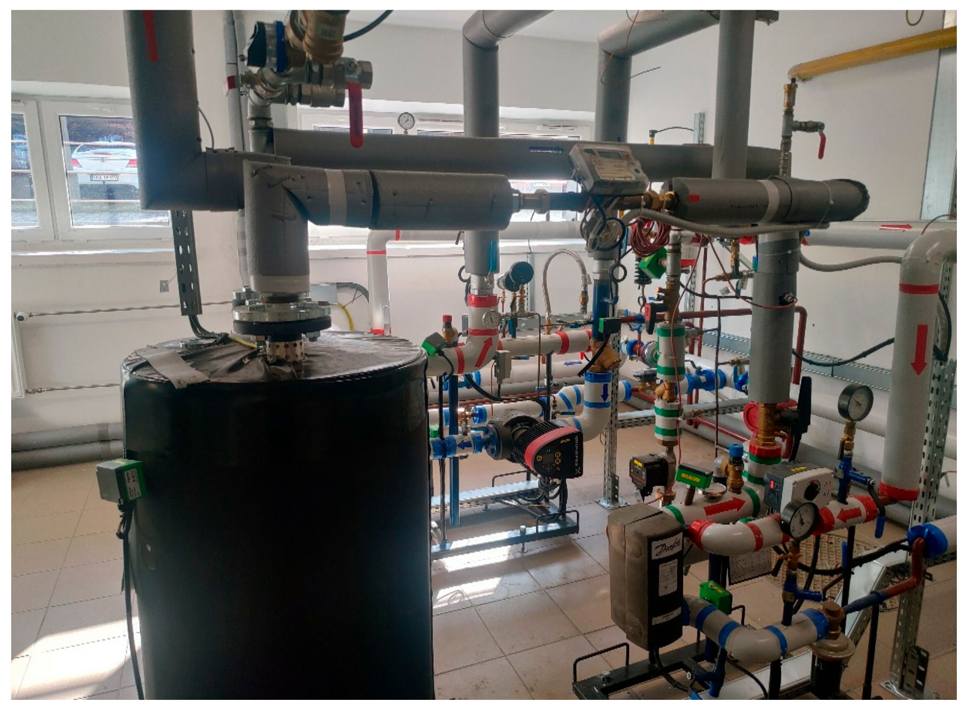
The research discussed in this article will be conducted at two laboratory stands. One is a district heating substation belonging to the Municipal Heat Engineering Company (MPEC) in Krakow, which has existed for many years in one of the Cracow University of Technology buildings (Figure 1). The other is a new laboratory stand, a heat substation located in the laboratory of the Department of Energy (DE) of the Cracow University of Technology (Figure 2 and Figure 3a).

The heating substation in the DE laboratory is a parallel substation supplying two heating systems: a domestic hot water system (with PHE 1 in Figure 2) and a central heating system (with PHE 2 in Figure 2). The substation is supplied with hot water from an individual heat source, an electric boiler of the company ELTERM of 15 kW. The hot water reservoir used during the tests consists of two storage tanks with a capacity of 800 litres. A Danfoss heat exchanger model XB12M-1-16 (composed of 16 plates) is installed in the central heating system. In comparison, a Hexonic heat exchanger model LC110-30-2 (consisting of 30 plates) is installed in the domestic hot water system (Figure 3a). A drawing of a single heat exchanger plate with dimensions is shown in Figure 3b, while Figure 3c shows the type of embossing on the plates (chevron). Both heat exchangers are used as counter-flows.

The flow rate of cold and hot fluid in the system is measured using axial turbine flow meters ranging from 4 to 160 L/min (measuring accuracy: ±3% of measured value). Water temperatures in the installation are measured using type K (NiCr-Ni) sheathed thermocouple sensors with an outer diameter of 1.5 mm class 1. Figure 2 shows the location of sensors for measuring the temperature and flow rate. The location of sensors in the hot water system with PHE 1 are as follows: Th1,1 and Th2,1—hot water temperature measurement at the inlet and outlet, Tc1,1 and Tc2,1—cold water temperature measurement at the inlet and outlet, and mc1 and mh1—cold and hot water flow rate measurement. The location of sensors in the central heating system with PHE 2 are as follows: Th1,2 and Th2,2—measure the hot water temperature at the inlet and outlet, Tc1,2 and Tc2,2—measure the cold water temperature at the inlet and outlet, and mc2 and mh2—measure the cold and hot water flow rate. Compact pressure sensors with piezo-resistive measuring cells with temperature compensation and a pressure membrane made of special steel, whose basic error is ±0.1% of the final value, are used to measure the pressure in the installation. In contrast, the pressure drop in the heat exchangers is measured using differential pressure transmitters whose error for the basic measuring range is less than 0.05%. All sensors used for the measurements are from Ahlborn. All sensor measurement data are recorded by Ahlborn’s ALMEMO logger. The ALMEMO system enables real-time visualisation of the data collected from the sensors, data logging and the generation of reports in tables and graphs. Flow rate control in both systems is achieved via control valves. The research described in detail in this article will be carried out at the second stand.

6. Computation of the Cold Fluid Heat Transfer Coefficient in the Clean Heat Exchanger Using Measurement Data

The proposed algorithm, which is a modification of the Wilson method, was verified by carrying out test computations. They used measured data from the heat exchanger in the domestic hot water system of the laboratory stand described in the previous section.

Measurements carried out during the laboratory tests included measurements of water temperature at the inlet and outlet of the heat exchanger, as well as flow rates of cold and hot water. The data sampling time during the measurements was 1 s. Cold and hot water physical properties were determined for the average temperature values at the inlet and outlet of the heat exchanger, separately for each fluid.

The domestic hot water system under study uses a Hexonic LC110-30-2 PHE, and its heat transfer area $A=3.3 {\mathrm{m}}^2$. The correction factor $F=1$, because the analysed heat exchanger is a counter-flow one.

The measurements were carried out so that the flow rate of cold water was constant (about 40 L/min.) while the flow rate of hot water was changed (in the range from about 5 to 40 L/min). From the archived database, $N=8$ measurement points were selected. At the beginning of the test calculations, the mean heat flow rates ${\dot{Q}}_m$ and overall heat transfer coefficients $k$ of the PHE under test were determined for a selected number of measurement points ($i=1,\dots , N$). The results of these calculations are shown in

Table 1. Selected measurement points from tests carried out on 12 May 2023 and computed values for the mean heat flow rate ${\dot{Q}}_m$ and the overall heat transfer coefficient $k$.

Time	$${\mathit{T}}_{\mathit{h}1}$$	$${\mathit{T}}_{\mathit{h}2}$$	$${\mathit{T}}_{\mathit{c}1}$$	$${\mathit{T}}_{\mathit{c}2}$$	$${\dot{\mathit{V}}}_{\mathit{h}}$$	$${\dot{\mathit{V}}}_{\mathit{c}}$$	$${\overline{\mathit{c}}}_{\mathit{w}\mathit{h}}$$	$${\overline{\mathit{c}}}_{\mathit{w}\mathit{c}}$$	$${\dot{\mathit{Q}}}_{\mathit{h}}$$	$${\dot{\mathit{Q}}}_{\mathit{c}}$$	$${\dot{\mathit{Q}}}_{\mathit{m}}$$	$$\mathit{\Delta }{\mathit{T}}_{\mathit{m}}$$	$$\mathit{k}$$
	°C	°C	°C	°C	L/min	L/min	J/(kgK)	J/(kgK)	W	W	W	K	W/(m2K)
11:46:50	63.7	57.4	12.6	63.6	40.1	4.9	4184.36	4178.60	17,319.2	17,279.2	17,299.2	7.32	715.94
11:49:49	62.9	50.2	12.2	61.2	40.1	10.2	4182.60	4178.61	34,969.7	34,575.6	34,772.7	11.68	901.89
11:54:34	60.6	43.3	12.0	56.3	39.7	15.0	4180.94	4178.76	47,245.9	46,010.8	46,628.3	13.60	1038.80
11:57:44	59.0	39.0	11.8	51.7	39.9	20.0	4180.09	4179.07	54,956.6	55,301.1	55,128.8	15.13	1104.21
12:00:10	56.9	34.9	11.6	46.5	39.8	24.9	4179.40	4179.61	60,371.0	60,278.8	60,324.9	15.99	1143.08
12:01:24	56.3	32.5	11.6	43.1	39.8	30.0	4179.14	4180.07	65,346.7	65,588.7	65,467.7	16.76	1183.96
12:03:09	54.8	29.6	11.4	40.0	39.7	34.8	4178.84	4180.61	69,072.5	69,118.1	69,095.3	16.44	1273.49
12:03:55	54.0	28.0	11.7	37.4	39.7	39.7	4178.73	4181.05	71,296.3	70,883.3	71,089.8	16.45	1309.60

.

Table 2. Average temperature values and physical properties of hot and cold water for selected measuring points from tests carried out on 12 May 2023.

Time	${\mathit{T}}_{\mathit{m},\mathit{h}}$	${\mathit{T}}_{\mathit{m},\mathit{c}}$	${\mathit{\rho }}_{\mathit{h}}$	${\mathit{\rho }}_{\mathit{c}}$	${\mathit{\nu }}_{\mathit{h}}$	${\mathit{\nu }}_{\mathit{c}}$	$\mathit{P}{\mathit{r}}_{\mathit{h}}$	$\mathit{P}{\mathit{r}}_{\mathit{c}}$	${\mathit{\lambda }}_{\mathit{h}}$	${\mathit{\lambda }}_{\mathit{c}}$
	°C	°C	kg/m3	kg/m3	×10−6 m2/s	×10−6 m2/s	-	-	W/(mK)	W/(mK)
11:46:50	60.6	38.1	983.0	992.8	0.4701	0.6775	2.96	4.48	0.651	0.626
11:49:49	56.6	36.7	985.0	993.3	0.4980	0.6959	3.16	4.61	0.647	0.624
11:54:34	52.0	34.2	987.2	994.2	0.5340	0.7317	3.42	4.88	0.643	0.621
11:57:44	49.0	31.8	988.5	995.0	0.5597	0.7686	3.60	5.16	0.639	0.618
12:00:10	45.9	29.1	989.8	995.8	0.5892	0.8140	3.82	5.51	0.636	0.614
12:01:24	44.4	27.4	990.4	996.2	0.6045	0.8450	3.93	5.75	0.634	0.611
12:03:09	42.2	25.7	991.3	996.7	0.6283	0.8770	4.11	6.00	0.631	0.609
12:03:55	41.0	24.6	991.8	997.0	0.6420	0.9006	4.21	6.18	0.630	0.607

lists the average values of the temperatures $T_{m,h}$ and $T_{m,c}$ and the water properties, i.e., densities ${\rho }_h$ and ${\rho }_c$, kinematic viscosities ${\nu }_h$ and ${\nu }_c$, Prandtl numbers $P{r}_h$ and $P{r}_c$ and heat transfer coefficients ${\lambda }_h$ and ${\lambda }_c$, for hot and cold water, respectively.

In the next step, the cold water Nusselt numbers $N{u}_{c,i}$ were calculated according to the modified Colburn correlation expressed by Equation (8). The initial values of the constants $C_{c1}^{\left(0\right)}$ and $C_{c2}^{\left(0\right)}$ in the first iterative loop for calculating the Nusselt number values $N{u}_{c,i}$ were taken as $C_{c1}^{\left(0\right)}=0.05$ and $C_{c2}^{\left(0\right)}=0$. The water’s physical properties were computed for the average temperature using [18]. The calculated values of the Nusselt number for the selected measurement points $N{u}_{c,i}$ are shown in

Table 3. List of selected measuring points from 12 May 2023 and calculated overall heat transfer coefficients $k_i$ and Nusselt numbers $N{u}_{c,i}$ of cold water ($i=1,\dots , 8$).

i	Time	${\mathit{T}}_{\mathit{h}1,\mathit{i}}$	${\mathit{T}}_{\mathit{h}2,\mathit{i}}$	${\mathit{T}}_{\mathit{c}2,\mathit{i}}$	${\mathit{T}}_{\mathit{c}1,\mathit{i}}$	${\dot{\mathit{m}}}_{\mathit{h},\mathit{i}}$	${\dot{\mathit{m}}}_{\mathit{c},\mathit{i}}$	$\mathit{\Delta }{\mathit{T}}_{\mathit{m},\mathit{i}}$	${\mathit{k}}_{\mathit{i}}$	$\mathit{N}{\mathit{u}}_{\mathit{c},\mathit{i}}$
		°C	°C	°C	°C	kg/s	kg/s	°C	W/(m2K)	-
1	11:46:50	63.7	57.4	12.6	63.6	0.657	0.081	7.32	715.94	1.284
2	11:49:49	62.9	50.2	12.2	61.2	0.658	0.169	11.68	901.89	2.282
3	11:54:34	60.6	43.3	12.0	56.3	0.653	0.249	13.60	1038.80	3.041
4	11:57:44	59.0	39.0	11.8	51.7	0.657	0.332	15.13	1104.21	3.748
5	12:00:10	56.9	34.9	11.6	46.5	0.657	0.413	15.99	1143.08	4.359
6	12:01:24	56.3	32.5	11.6	43.1	0.657	0.498	16.76	1183.96	4.980
7	12:03:09	54.8	29.6	11.4	40.0	0.656	0.578	16.44	1273.49	5.520
8	12:03:55	54.0	28.0	11.7	37.4	0.656	0.660	16.45	1309.60	6.064

. In Table 3 et seq., $i$ denotes the number of measurement points in the sequence.

Then, the cold-side heat transfer coefficients ${\alpha }_{c,i}$ of the heat exchanger were calculated using Equation (9), and later, the hot-side heat transfer coefficients ${\alpha }_{h,i}^{\prime }$ were calculated using Equation (10). In order to calculate ${\alpha }_{h,i}^{\prime }$, it is necessary to know the thickness of the plates in the heat exchanger, which is ${\delta }_p=0.001 \mathrm{m}$, and the thermal conductivity of the material from which they are made (stainless steel), which is ${\lambda }_p=16 \mathrm{W}/\left(\mathrm{mK}\right)$. In the next step, based on Equation (11), the values of the Nusselt number for hot water $N{u}_{h,i}^{\prime }$ were determined, which were then approximated by the linear function (12), which allowed us to determine the constants $C_{h1}^{\left(1\right)}$ and $C_{h2}^{\left(1\right)}$, the values of which are −0.23977 and 40.00581, respectively.

The results of the subsequent calculations listed above needed to calculate the constants $C_{h1}^{\left(1\right)}$ and $C_{h2}^{\left(1\right)}$ are shown in

Table 4. Results of first iteration calculations for $i=1,\dots , 8$ measurement points to determine the constants $C_{h1}^{\left(1\right)}$ and $C_{h2}^{\left(1\right)}$.

i	${\mathit{k}}_{\mathit{i}}$	$\mathit{N}{\mathit{u}}_{\mathit{c},\mathit{i}}$	${\mathit{\alpha }}_{\mathit{c},\mathit{i}}$	${\mathit{\alpha }}_{\mathit{h},\mathit{i}}^{\prime }$	$\mathit{N}{\mathit{u}}_{\mathit{h},\mathit{i}}^{\prime }$	$\mathit{R}{\mathit{e}}_{\mathit{h},\mathit{i}}$	$\mathit{P}{\mathit{r}}_{\mathit{h},\mathit{i}}$
	W/(m2K)	-	W/(m2K)	W/(m2K)	-	-	-
1	716	1.284	651	−4002	−7.58	344.42	2.96
2	902	2.282	1154	7630	14.55	325.11	3.16
3	1039	3.041	1530	5062	9.72	300.15	3.42
4	1104	3.748	1876	3830	7.39	287.82	3.60
5	1143	4.359	2168	3311	6.43	272.72	3.82
6	1184	4.980	2466	3052	5.94	265.81	3.93
7	1274	5.520	2722	3263	6.38	255.10	4.11
8	1310	6.064	2982	3157	6.18	249.65	4.21

. Table 4 also contains the values of the Reynolds $R{e}_{h,i}$ and Prandtl $P{r}_{h,i}$ numbers of hot water necessary to perform the approximation with a linear function.

In Table 4, for the first measurement point, the heat transfer coefficient ${\alpha }_{h,i}^{\prime }$ and the Nusselt number $N{u}_{h,i}^{\prime }$ have negative values. This only occurs in the first iteration and is due to the fact that when determining ${\alpha }_{h,i}^{\prime }$ from Equation (10), the sum of the heat transfer resistance on the cold side and heat conduction was larger than the total heat transfer resistance of the heat exchanger. Therefore, ${\alpha }_{h,i}^{\prime }$ in this case has a negative value. The Nusselt number $N{u}_{h,i}^{\prime }$ was determined from the ${\alpha }_{h,i}^{\prime }$ of Equation (11), so its value is also negative. The problem was eliminated in subsequent iterations, due to the increasingly better fit of the constants in the Nusselt number correlations.

After determining the constants $C_{h1}^{\left(1\right)}$ and $C_{h2}^{\left(1\right)}$, the Nusselt numbers $N{u}_{h,i}$ from Equation (12) were again determined, and from them, the heat transfer coefficients ${\alpha }_{h,i}$ from Equation (13) were calculated, followed by the heat transfer coefficients ${\alpha }_{c,i}^{\prime }$ from Equation (14). The Nusselt number values for cold water $N{u}_{c,i}^{\prime }$ were then computed from Equation (15). The results of the calculations are presented in

Table 5. Results of first iteration calculations for $i=1,\dots ,8$ measurement points to determine the constants $C_{c1}^{\left(1\right)}$ and $C_{c2}^{\left(1\right)}$.

i	${\mathit{k}}_{\mathit{i}}$	$\mathit{N}{\mathit{u}}_{\mathit{h},\mathit{i}}$	${\mathit{\alpha }}_{\mathit{h},\mathit{i}}$	${\mathit{\alpha }}_{\mathit{c},\mathit{i}}^{\prime }$	$\mathit{N}{\mathit{u}}_{\mathit{c},\mathit{i}}^{\prime }$	$\mathit{R}{\mathit{e}}_{\mathit{c},\mathit{i}}$	$\mathit{P}{\mathit{r}}_{\mathit{c},\mathit{i}}$
	W/(m2K)	-	W/(m2K)	W/(m2K)	-	-	-
1	716	3.273	1727	1416	2.79	31.15	4.48
2	902	4.171	2188	1851	3.66	63.13	4.61
3	1039	5.504	2866	1991	3.96	88.28	4.88
4	1104	6.054	3136	2104	4.20	112.07	5.16
5	1143	6.857	3533	2082	4.19	131.74	5.51
6	1184	7.217	3708	2157	4.36	152.90	5.75
7	1274	7.818	4000	2360	4.78	170.89	6.00
8	1310	8.112	4141	2435	4.95	189.85	6.18

.

The first iteration ends with the approximation of the calculated values of the Nusselt numbers $N{u}_{c,i}^{\prime }$ by Equation (8) using the linear regression method, resulting in the constants $C_{c1}^{\left(1\right)}$ and $C_{c2}^{\left(1\right)}$, which are 0.01988 and 2.55663, respectively. The coefficient of determination of the approximation using the linear function (8) performed is $r^2=0.9314202$. The approximation using the linear function (8) is also shown graphically in Figure 4. The computed constants $C_{c1}^{\left(1\right)}$ and $C_{c2}^{\left(1\right)}$ are the initial values for the next iteration loop.

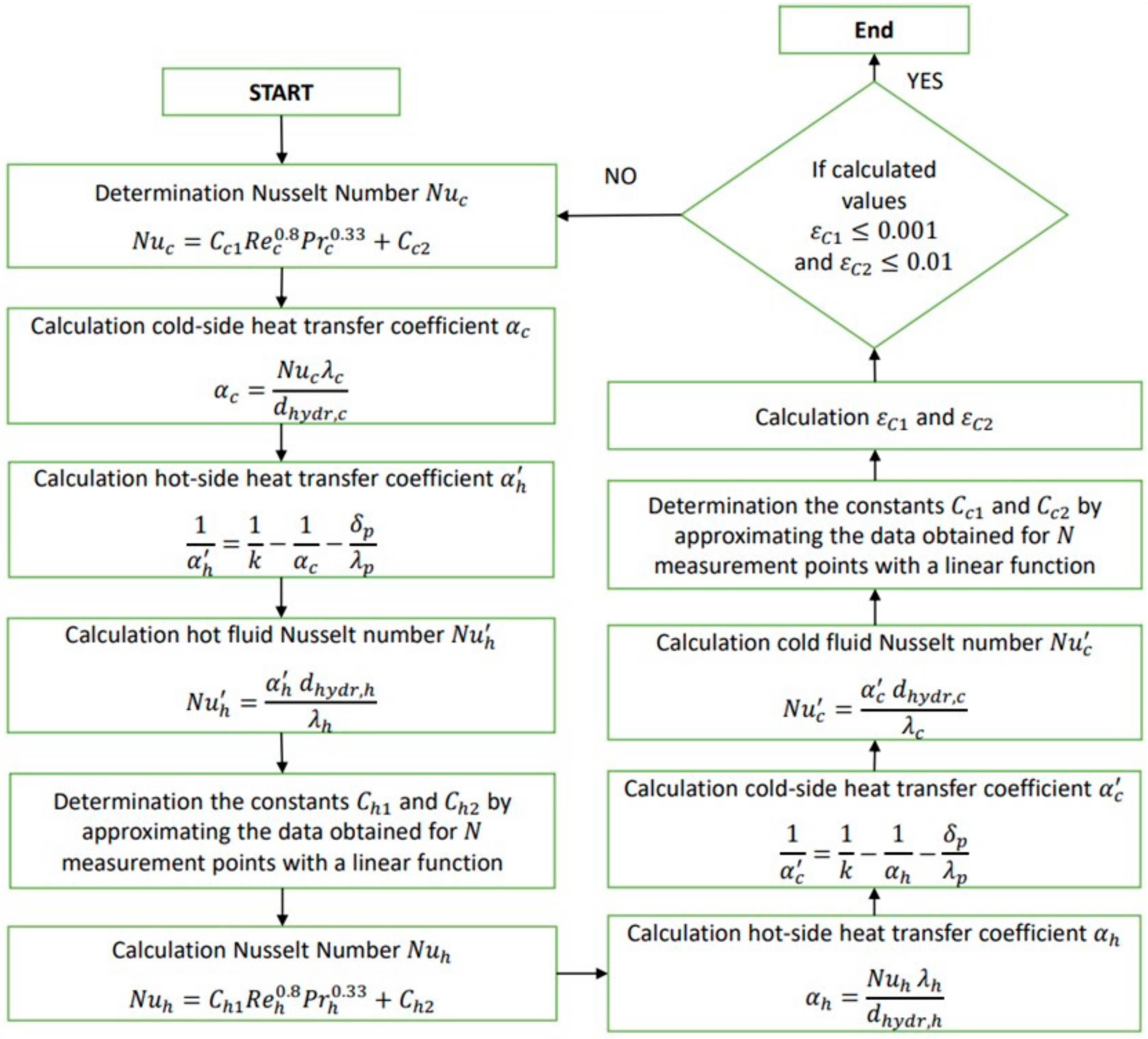
The computational algorithm for determining the Nusselt number correlation for a cold fluid is shown as a block diagram in Figure 5.

Table 6. Calculated values of Nusselt numbers $N{u}_{c,i}$ and heat transfer coefficients ${\alpha }_{c,i}$ in five subsequent iterations.

	Iteration Number (j)
	(1)		(2)		(3)		(4)		(5)
i	$\mathit{N}{\mathit{u}}_{\mathit{c},\mathit{i}}$	${\mathit{\alpha }}_{\mathit{c},\mathit{i}}$	$\mathit{N}{\mathit{u}}_{\mathit{c},\mathit{i}}$	${\mathit{\alpha }}_{\mathit{c},\mathit{i}}$	$\mathit{N}{\mathit{u}}_{\mathit{c},\mathit{i}}$	${\mathit{\alpha }}_{\mathit{c},\mathit{i}}$	$\mathit{N}{\mathit{u}}_{\mathit{c},\mathit{i}}$	${\mathit{\alpha }}_{\mathit{c},\mathit{i}}$	$\mathit{N}{\mathit{u}}_{\mathit{c},\mathit{i}}$	${\mathit{\alpha }}_{\mathit{c},\mathit{i}}$
	-	W/(m2K)	-	W/(m2K)	-	W/(m2K)	-	W/(m2K)	-	W/(m2K)
1	1.284	651.39	3.067	1556.28	3.012	1528.46	2.962	1503.04	2.917	1480.23
2	2.282	1154.34	3.464	1752.46	3.426	1733.04	3.390	1715.18	3.358	1699.00
3	3.041	1529.81	3.766	1894.62	3.740	1881.61	3.716	1869.50	3.694	1858.38
4	3.748	1875.73	4.047	2025.23	4.033	2018.13	4.019	2011.33	4.007	2004.87
5	4.359	2167.46	4.290	2133.15	4.286	2131.09	4.281	2128.84	4.276	2126.37
6	4.980	2465.99	4.537	2246.62	4.543	2249.64	4.548	2251.95	4.551	2253.49
7	5.520	2722.05	4.751	2343.25	4.766	2350.64	4.779	2356.89	4.789	2361.89
8	6.064	2981.92	4.968	2442.90	4.992	2454.69	5.013	2464.88	5.030	2473.35

shows the calculated Nusselt numbers $N{u}_{c,i}$ and heat transfer coefficients ${\alpha }_{c,i}$ for cold water in five successive iteration steps.

The computational results of the successive iterations presented in Table 6 show that the proposed iterative method converges. The values of the constants $C_{c1}^{\left(j\right)}$ and $C_{c2}^{\left(j\right)}$ determined in subsequent iterations and the coefficients of determination $r^2$ are summarised in

Table 7. Values of $C_{c1}^{\left(j\right)}$ and $C_{c2}^{\left(j\right)}$ and the coefficients of determination $r^2$ for successive iterations.

j	${\mathit{C}}_{\mathit{c}1}^{\left(\mathit{j}\right)}$	${\mathit{C}}_{\mathit{c}2}^{\left(\mathit{j}\right)}$	${\mathit{r}}^2$
1	0.01988	2.56	0.93142
2	0.02071	2.48	0.93501
3	0.02145	2.41	0.91899
4	0.02210	2.35	0.94114
5	0.02266	2.30	0.94367
6	0.02313	2.25	0.94587
7	0.02353	2.21	0.94776
8	0.02386	2.17	0.94938
9	0.02412	2.14	0.95076
10	0.02434	2.12	0.95194
11	0.02451	2.09	0.95294
12	0.02464	2.07	0.95381
13	0.02474	2.06	0.95455
14	0.02482	2.04	0.95519
15	0.02488	2.03	0.95574
16	0.02491	2.02	0.95623
17	0.02493	2.01	0.95666
18	0.02494	2.00	0.95704
19	0.02494	1.99	0.95739
20	0.02493	1.98	0.95770

and shown graphically in Figure 6a,b.

The modified Wilson method described in this article enables the determination of constants in the correlation of the Nusselt number for cold fluid flowing through a heat exchanger. Both conditions (16) and (17) were satisfied after 17 iterations. The final form of the correlation for the Nusselt number for cold water, when the hot water flow rate is about 40 L/min, is as follows:

$$N{u}_c=0.02493R{e}_c^{0.8}P{r}_c^{0.33}+2.01 \mathrm{for} 30 \le R{e}_c\le 190$$

(18)

However, it can also be used to determine the constants in the correlation of the Nusselt number of a hot fluid, but this will require subsequent measurements in which the hot fluid flow is constant and the cold fluid flow is variable.

7. Conclusions

This paper presents a method for determining the thermal resistance of fouling of PHEs in district heating substations and a method for determining the correlation of the Nusselt numbers of cold and hot fluid flowing through a clean heat exchanger (and, indirectly, the thermal resistance of the apparatus). The computational test of the second method was carried out for the measurement data obtained on a laboratory stand specially built for this purpose, which is a district heating substation of the domestic hot water system. Several iterations were carried out, and the method gave good results because they converged. As the final result of the presented research, a correlation with the Nusselt number for cold water flowing through the heat exchanger was obtained. It will allow us to determine the heat transfer coefficient on the cold side of the heat exchanger for each of its operating conditions.

The developed method will allow us to assess the degree of contamination of the PHEs. The method is fast and simple to use in practice. It will enable us to monitor the operation of PHEs in district heating substations and optimise heat exchanger cleaning intervals.