Article

Application of the Time-Domain Signal Analysis for Electrical Appliances Identification in the Non-Intrusive Load Monitoring

1
Institute of Radioelectronics and Multimedia Technologies, Warsaw University of Technology, Nowowiejska 15/19, 00-665 Warsaw, Poland
2
Institute of Electrical Power Engineering, Warsaw University of Technology, Koszykowa 75, 00-662 Warsaw, Poland
*
Author to whom correspondence should be addressed.
Energies 2022, 15(9), 3325; https://doi.org/10.3390/en15093325
Submission received: 1 April 2022 / Revised: 25 April 2022 / Accepted: 30 April 2022 / Published: 3 May 2022
(This article belongs to the Section A1: Smart Grids and Microgrids)

Abstract

:
The paper presents a novel method for non-intrusive appliances identification. It can be used for energy load disaggregation in a smart grid. The approach identifies changes in the state of the particular appliance by measuring and processing the common supply current signal. Analysis of the instantaneous changes in the aggregated current on the output of the analyzed circuit in the power network is exploited here. The signal is processed using the time alignment of the current and voltage signals samples represented in the array form. The scheme includes filtering, event detection and identification, which is performed by comparing parameters of the detected event against previously determined signatures of monitored appliances. The analysis is performed in the time domain; therefore (unlike other existing methods), the information contained in the original signal is not lost. The approach was tested in the laboratory designed specifically for this purpose. All tests have been conducted with up to 12 appliances operating at the same time in the single power supply circuit. The measurement setup was developed and used to record appliances’ switching on/off events. During tests, 2300 events for devices were recorded. Collected data were processed to identify particular devices with the accuracy of 98.8% and macro-averaged F-score measure of 0.9874. High identification accuracy was achieved despite the high number of devices operating in the background.

1. Introduction

Accurate energy management, including load disaggregation in the end-user area, allows for reducing the energy demand during peak loads. This can be achieved by the information derived from NILM (Non-Intrusive Load Monitoring) analysis. The aim of such systems is to determine the operational state of electrical Energy Appliances (EA) in the selected time instants and estimate their energy consumption in the long term through disaggregation. In the NILM concept (proposed in 1992 [1]), the sources of information for the appliance identification are aggregated currents and voltages measured in a single location, near the energy meter. From these signals, various features (such as power or impedance) are extracted. This way, each appliance may be represented as a vector of characteristic parameters describing its state. Analysis of such vectors leads to knowledge extraction by Machine Learning (ML) methods [2]. It was shown that the feedback information from such systems may lead to decrease in the energy consumption by 12% [3].
In this paper, a novel method for the appliance identification is proposed. It exploits the analysis of the current and voltage signal samples during the time of 20 ms (for a 50 Hz network), which is the period of the fundamental harmonic of the power signal. The method for processing the current signal allows for extracting signal components carrying device-specific information that are short-lived relative to the period of the fundamental component. First, periodicity of the network voltage is exploited. It allows for dividing the signal into separate periods (for instance, by assuming the beginning of the period as the time instant of the fundamental component’s zero crossing). From them, the array-like representation of the current samples is constructed. It allows for the current signal filtering in terms of the fundamental component, reducing the noise level of the appliance signature. The latter is determined residually, i.e., by subtracting signal samples from periods before and after the change of the device’s state. The analysis is performed in the time domain, unlike other known methods. The method for transforming and filtering the signal was developed, to make our approach resilient to the number and configuration of appliances operating in the background, which was the main purpose of this study. The influence of the signal sampling rate and filter order of the proposed signal processing method on the identification accuracy were analyzed.
To identify devices, a large number of scenarios must be considered. For this task, the modified measurement system [2] was used to record 2300 events (turning appliances on and off). The content of the paper is as follows. In Section 2, works related to non-invasive load monitoring in households are reviewed. Section 3.1 covers the applied measurement system for data collection. In Section 3.2, the method for calculating the appliance’s current signature is presented. Section 3.3 covers the proposed algorithm for the detection and identification of appliance’s states. Obtained results are in Section 4, while in Section 5, the summary and future prospects are presented.

2. State of the Art

Numerous NILM methods (developed since the 1980s) differ in sampling frequency, extracted characteristics and identification methods. All have limitations (are useful for a certain class of receivers, may be constrained to EA with switched-mode power supply, etc.); therefore, new approaches must be investigated. According to the NILM systems classification presented in [2,4,5,6,7,8], the main taxonomy criterion is the sampling frequency fs of the current signal. Three groups of algorithms may be distinguished:
  • LF (Low Frequency) group where signals are measured with fs between fractions of the single Hz and 50 Hz;
  • MF (Medium Frequency) group, where fs is between 1 and 90 kHz;
  • HF (High Frequency) group, with fs between tens of kHz and single MHz.
The last one was introduced for the analysis of high-frequency disturbances, which were generated by the specific group of appliances (such as motor-driven devices or with the switched-mode power supply) [9]. The general NILM architecture is presented in Figure 1. Its crucial components include signal acquisition and characteristic features (symptoms) extraction modules. Based on the symptoms’ changes, the appliance identification module discovers the device that changed its state (further called appliance recognition). To detect the state change (event), the calculated feature vector is compared to the set of stored signatures (dictionary entries). Each entry is obtained from measurements taken in the controlled conditions for the single device operating in the network with all others switched off.
Virtually all appliance identification methods [2] are based on the analysis of measured physical quantities, averaged for the multiplicity of the fundamental component’s period in the network. In the case of the LF group, acquired quantities may be the Root Mean Square (RMS) value of the current or the active power for signals recorded with the frequency up to 50 Hz. In older LF methods, appliance signatures include changes in the value of the consumed current after the state change [10,11,12,13,14]. Since 2018, NILM publications utilizing deep Artificial Neural Networks (ANN) dominate the field for low-frequency data [6,15,16,17], as well as methods based on hidden Markov chains [18,19]. Typically, the active power P [6] is analyzed. The HF Group covers methods based on the analysis of high-frequency disturbances in the voltage and current signals [20,21]. Here, signature elements include parameters describing changes in the spectrum after changing the appliance’s state [9]. The disaggregation is performed based on the FFT (Fast Fourier Transform) output analysis. Even when STFT (Short-Time Fourier Transform) is applied, information about the time instant of the sample’s value changes is lost (only frequency components remain). Partly, this problem can be solved by using the Wavelet Transform (WT), which uses a variable-width analysis window [21,22]. The NILM methods using WT are vulnerable to changes in the background signal [22].
In the MF group, to which the method described in this paper belongs to, the typical features are current harmonic components [23,24,25], which are often calculated using FFT for the window of a couple of milliseconds duration. The short-term, non-zero values of the higher harmonic components are therefore averaged, and the information carried by them is suppressed.
The method proposed in this paper is most similar to approaches exploiting the voltage–current (V-I) trajectory analysis, which was first introduced in [26]. Initially, classification was based on features extracted from shapelets such as looping direction, number of intersections or enclosed area [27]. Additional features were used in [28]. As a result, information about the time instants of the samples values’ changes in the cycle is lost.
Analogically, in the MF group, there was also a significant increase in the use of deep ANN. The image representation of V-I trajectories is exploited in [29]. Later publications proposed including more information from images analyzed by ANN [30]. In [31,32], a new way of creating classified images based on V-I trajectories was proposed, with Adaptive Weighted Recurrence Graph (AWRG) blocks. The Fryze power theory and Euclidean distance similarity function were applied in [33]. The only method where both time and frequency domain information is preserved is [34]. In their model, the Gramian Angular Field (GAF) matrices and Markov Transition Field (MTF) algorithms were used to encode the static and dynamic current series information in the time domain.
In addition to the loss of information about the time instants of the values’ changes inside the cycle, we see additional risks in the above MF methods. Most of them are verified against popular data sets [35] acquired using submeters for each appliance or having only up to two devices active in the background, such as PLAID [30,31,32,33,34] and WHITED [30,32].
The number of appliances working in the background during the analysis affects the quality of the appliance identification. The same is with V-I trajectories used as the source of features. Simulated scenarios from known data sets [36] are not suited for real-world data processing, as they do not represent the influence of devices other than those being aggregated (for example, operating in the standby mode). Depending on the measurement technology, differences in the voltage signal and noise level may occur [37]. Decreasing accuracy with the increase in the number of devices working in the background is a serious concern [10,33,38,39,40].
In this paper, the method for transforming the current signal to an array-like representation is proposed. To some extent, a similar approach was used in [41], where analysis of the graphical representation of the transient state with ANN was conducted. Contrary to that approach, we do not have to resample the voltages and interpolate the currents. Our signal processing method (especially filtering) allows for de-noising and stabilizing the signal. This way, the high identification accuracy is maintained, despite the increasing number of appliances operating in the background.

3. Test Stand and Methods

3.1. Laboratory Test Stand and Experiments

The proposed measurement system (Figure 2) based on [
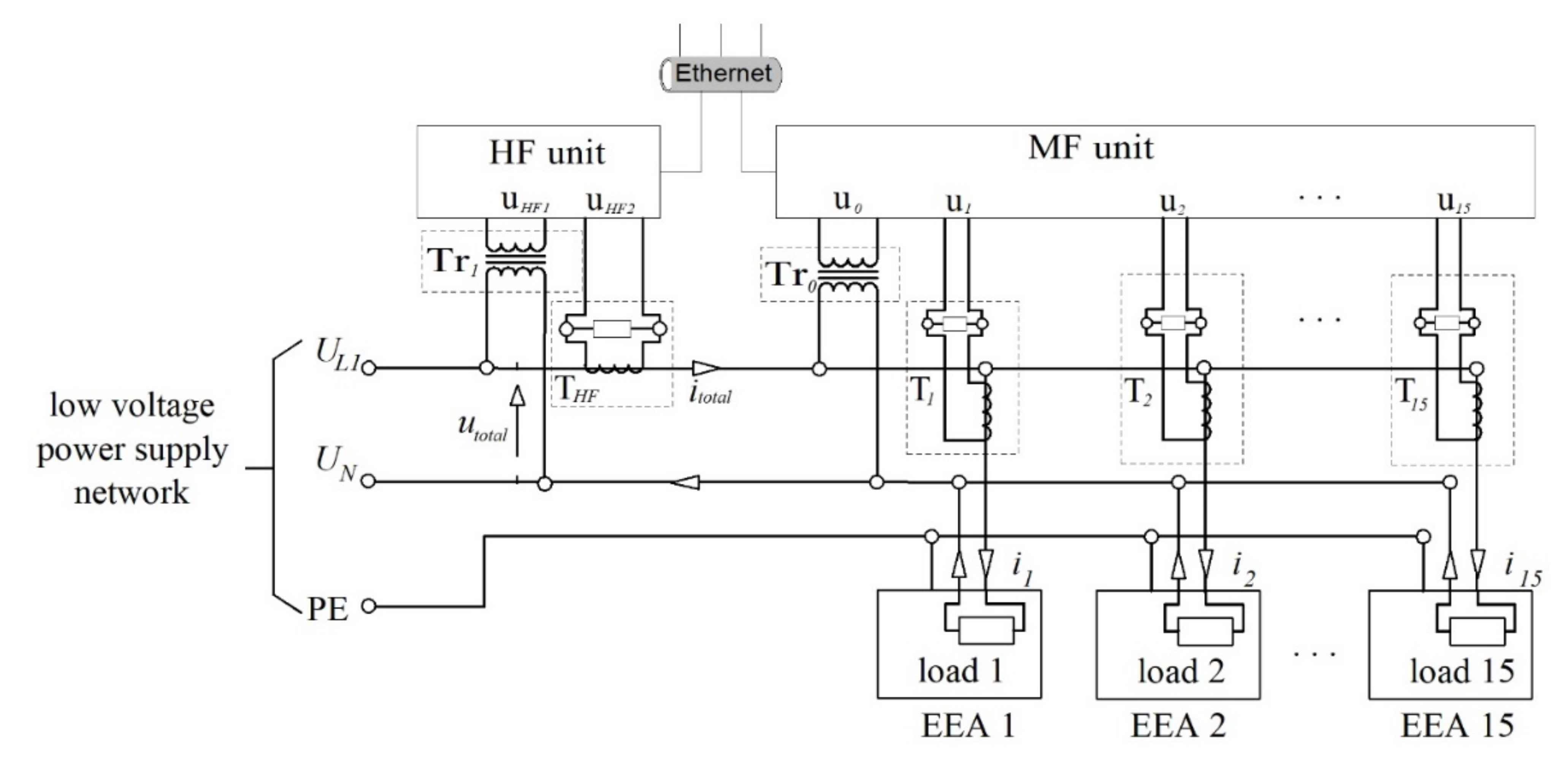
2] allows for performing Data Acquisition (DAQ) with the frequency between a couple kHz to a single MHz. It consists of two computers working as DAQ modules and software for processing the collected data. The first computer (MF unit) is used to acquire samples with the frequency f s = 62.5 kHz on 16 channels simultaneously with 16-bit resolution. The second computer (HF unit) allows for the DAQ with f s up to 10 MHz on two channels at the same time, with the 12-bit resolution. Signals representing values of the total current in the main power line u H F 2 t and the j -th socket ( j 1 , 15 ) u j t are measured using the current transformers (indicated in Figure 2 as T H F   and T j ).
The key for automatically describing measurement data is the simultaneous current measurement for each appliance connected to the network. In the presented system, it is possible thanks to sensors attached to each socket. The MF unit allows for acquiring samples of currents consumed by the particular appliances connected to sockets. The identification algorithms use data derived from the aggregated current i t o t a l (signal   u H F 2 ) and supply voltage u t o t a l (signal u H F 1 ).
Measurements by both computers (MF and HF) are implemented in the LabVIEW-based software [2]. In the HF setup, measurements are performed with f s H F   = 250 kHz, while for the MF, f s M F =12.5 kHz. Descriptions of the measured data (labeling the actual appliances state in the particular time instants) are added automatically after acquisition using the Matlab script. Characteristics of the measured appliances (including the number of events recorded during the laboratory tests) are in Table 1. The column “ a ” contains the appliance identifier. The column “Number of events” presents the number of events recorded during laboratory tests, which is caused by the change of this particular appliance’s state.
Experiments were conducted for 15 typical devices used in the household. In our research, we focused on two-state appliances, as it is easy to determine their actual configuration, enabling unambiguous verification of the results. In the case of multi-state appliances (such as a washing machine or dishwasher), it is often difficult to isolate their specific operational states. The fridge measured on channel no. 14 was not identified, working constantly in the background to verify the ability of the EA identification with additional signal components present. The fridge operation is characterized by the periodical changes in the current consumption.
The problem of identifying appliances with the non-zero background was introduced in [38]. Disaggregation algorithms in the configuration of multiple devices working simultaneously were considered in [42,43,44] but disregarding the influence of the background on the appliances’ identification. This makes the proposed research the next step of the NIALM systems’ development.
The data collection consisted of repeatedly turning the single device on or off and acquiring samples related with the state change. As a result, the training data set was created, containing examples representing particular events with the following elements:
  • Event type (on or off);
  • The actual device identifier;
  • Time instant of the event occurrence;
  • Recorded current samples;
  • Recorded supply voltage samples;
  • Other information regarding the appliance identification methods (such as the number and type of appliances operating in the background).
To include all appliances into the data set, the currents were measured in all sockets simultaneously. During the online implementation, the information about the sockets to which the devices are connected is not given, but during the training, the actual configuration of the network is known.

3.2. Appliance Signature Construction

During the stable operation of the appliance, the recorded instantaneous current values repeat in the periodically recurring time instants ( t m ). The period is determined using the timestamps t 0 k , i.e., the moments when the fundamental voltage component crosses zero (changes from negative to positive). The index k 
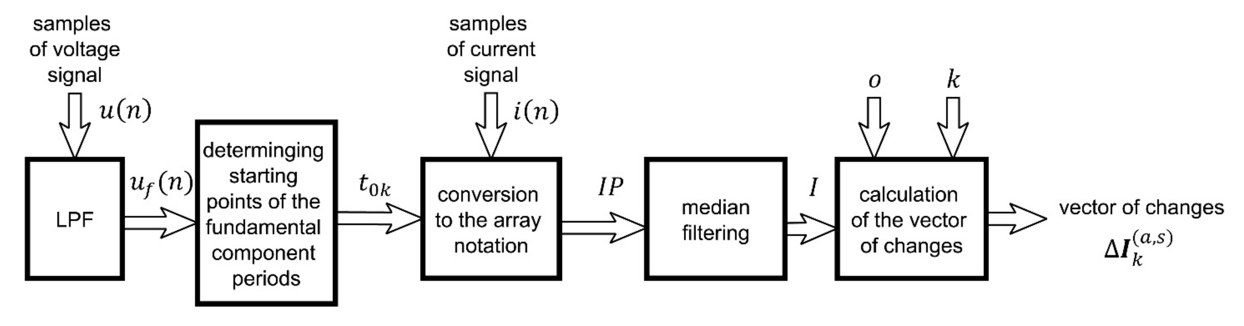
is number of the period in the supply voltage fundamental component. When adding the appliance to the network, turning it on or off, or changing its state, the instantaneous values of the current change. Steps required to extract the vector of changes Δ I k a , s occurring in the k -th period are presented in Figure 3. To describe the event, u n and i n samples are needed. They are the result of sampling signals i t o t a l t and u t o t a l t by the HF unit (see Figure 2).
The proposed method can be used independently of the supply voltage frequency, so it is applicable for both European and American households. The idea is to determine the difference between instantaneous values of the current in the specific periods of the voltage fundamental component, which were measured at the time instants t m in different periods k . The nominal frequency of the supply network signals is assumed constant, but in practice, small changes are present around fractions of the single Hz [45]. To suppress any deviations, the time instant t 0 k must be determined for each consecutive period. The proper selection of time instants t 0 k requires low-pass filtering (LPF in Figure 3) of the original voltage signal u n with the cut-off frequency of 70 Hz, outputting the signal u f n 
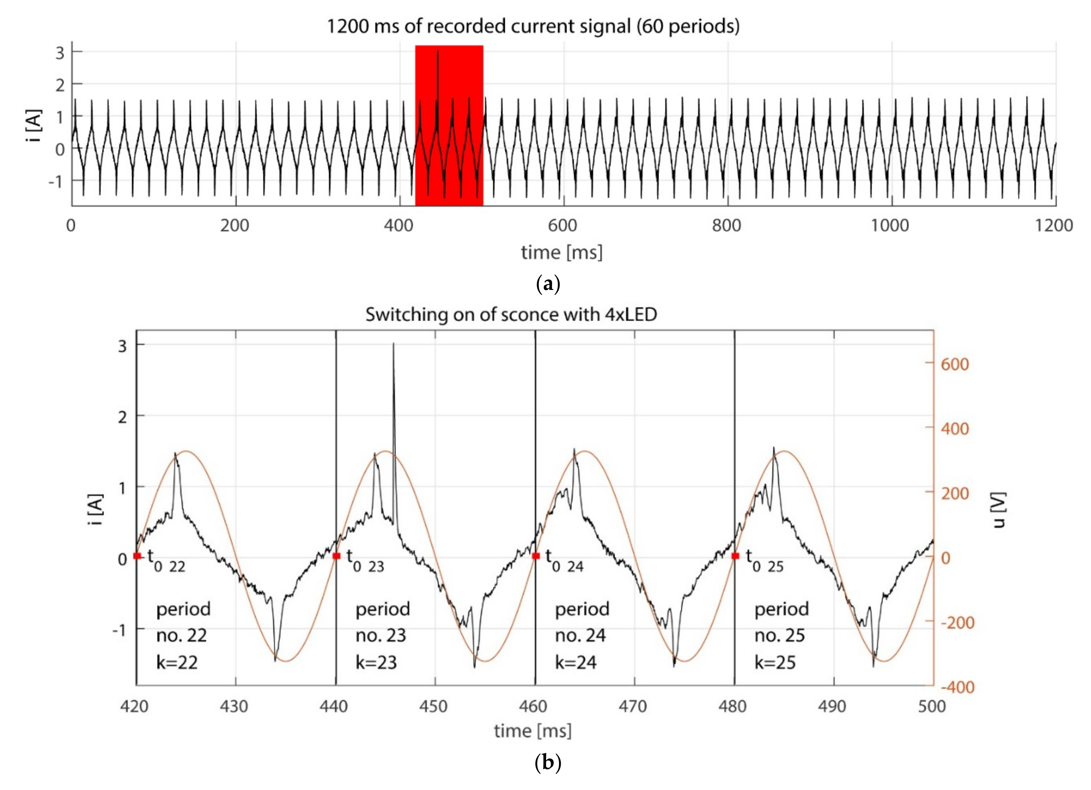
. This is needed to eliminate the influence of harmonics higher than the fundamental component. In Figure 4a, the current pattern during the event of turning the sconce with four LED bulbs on (device with identifier a = 3) is presented. The method for extracting the appliance signature from the red fragment of Figure 4a is in Figure 4b. Time instants t 0 k , for which the voltage samples u f n change signs from negative to positive are indicated by red dots. They show initial moments for subsequent periods k . Here, the turn-on event is detected in the 23rd period.
Time instants t 0 k are used for transforming collected current samples i n into the array I P . Its particular elements represent the instantaneous current values occurring in the same time position within each period k = 1 , , K . The latter contains M samples, which are identified by the index m . The period’s duration is 20 ms (50 Hz supply voltage) for the sampling frequency fs = 24,900 Hz, while the IP array contains M = 24900   H z 50   H z = 498 
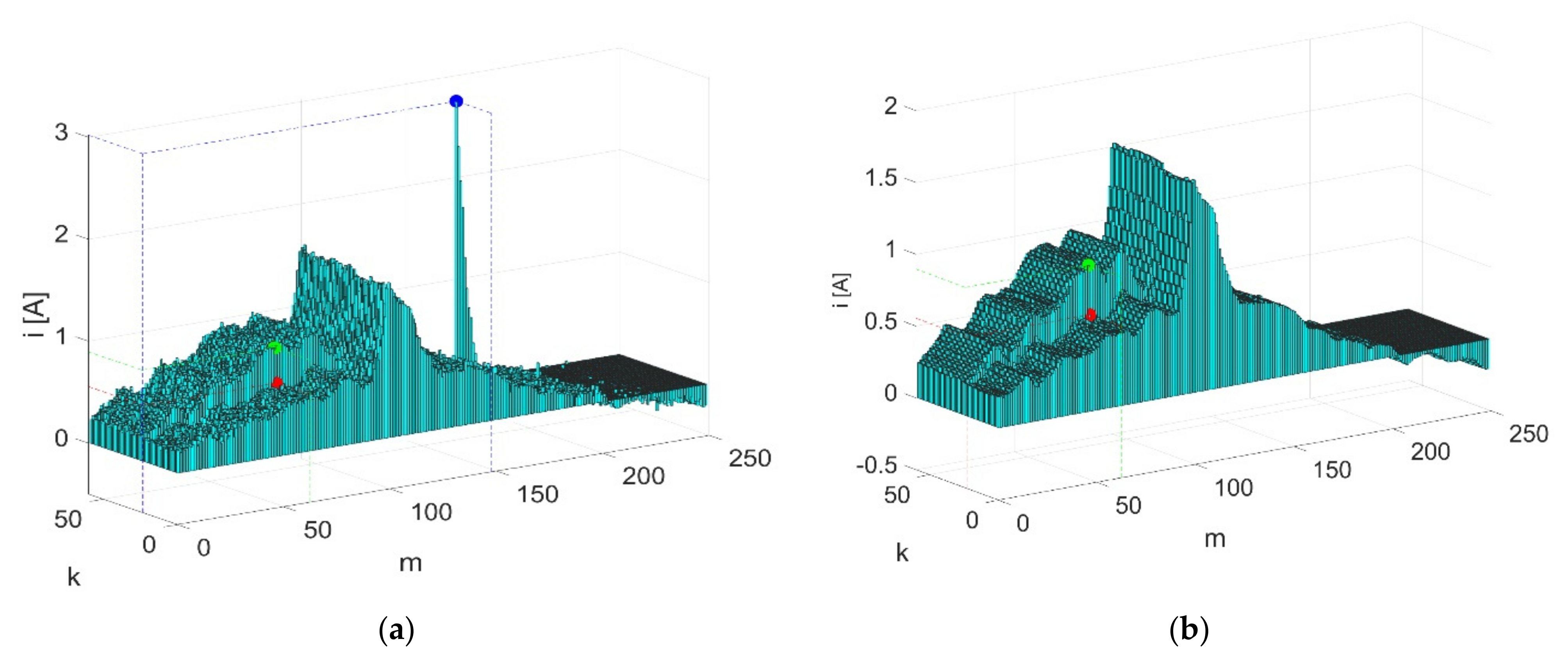
rows, each processed by the median filter (of the 15th order), leading to the array I .  
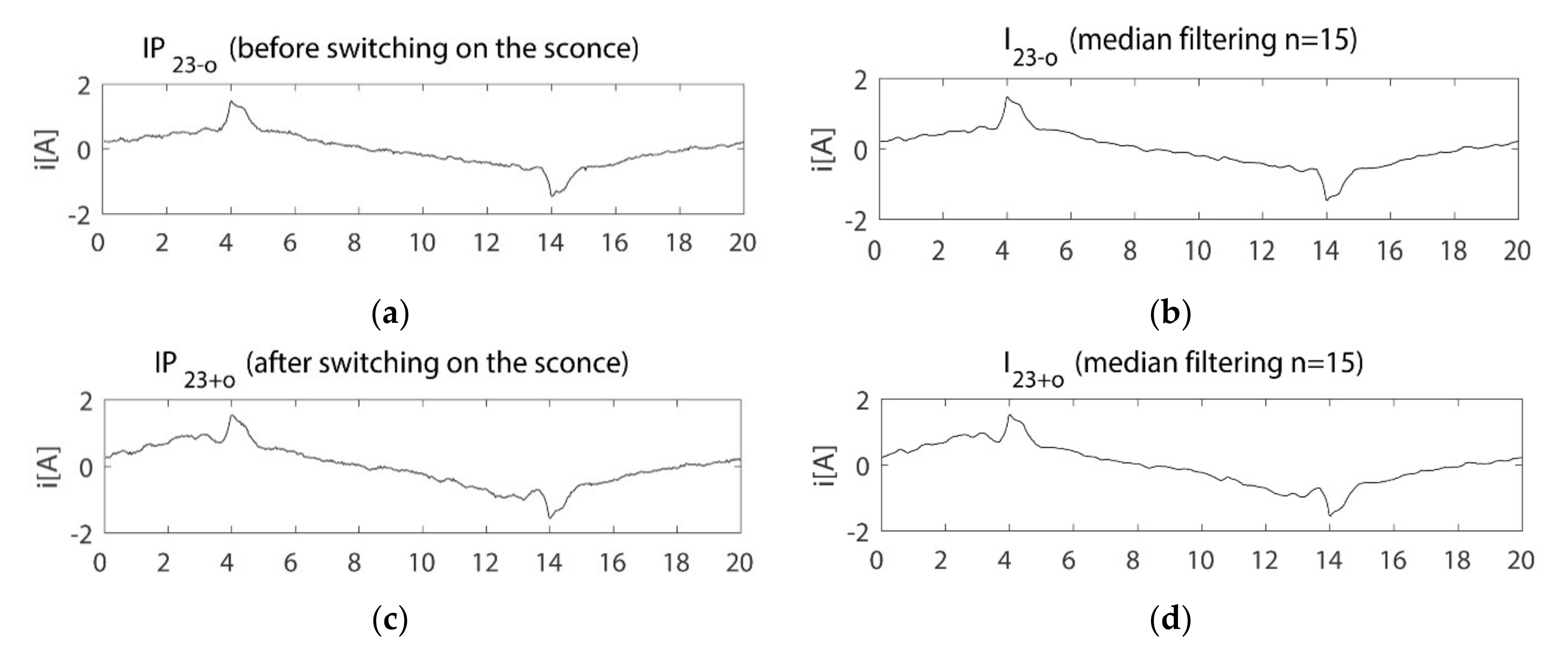
Figure 5a presents the first 250 samples in each row of I P , while Figure 5b shows corresponding rows I k (1) of I . These constitute the first halves of the current periods (see Figure 4a). Comparison between Figure 5a,b shows the effect of the median filtering (elimination of the high pitch indicated by the blue dot). Differences between two neighboring periods ( k = 23 and 24) reveal changes in the instantaneous current values caused by the appliance state change (the respective green and red dots).
I k = i 1 , k , , i m , k , , i M , k
The last step is determining the vector of changes Δ I k a , s (2) after the appliance state change. For this purpose, the difference between vectors equally distant in time from the k -th vector of the array I is calculated. The distance (number of periods) is defined by the value o 15 , 30 , 60 , 120 set individually (see Table 2 and Table 3) for each of a appliances (a = 1, …, A). It is obtained by subtracting samples of all periods’ pairs (such as k = 1 and k = 2, k = 3 and k = 5 and so on) in the steady state of the appliance operation. The difference Δ i m , k (3) is calculated for each sample m in the periods preceding (k − o) and succeeding (k + o) the period of interest (k).
Δ I k a , s = I k + o I k o   ,   f o r   k   N     k     o + 1 , K o
Δ i m , k = i m , k + o i m , k o  
The set of changes Δ I k a , s is the feature vector, which is used to classify the appliance’s state s . It is identified by comparing the currently analyzed vector and all dictionary entries Δ I p a t t e r n a , s representing appliances recognized in the network. 
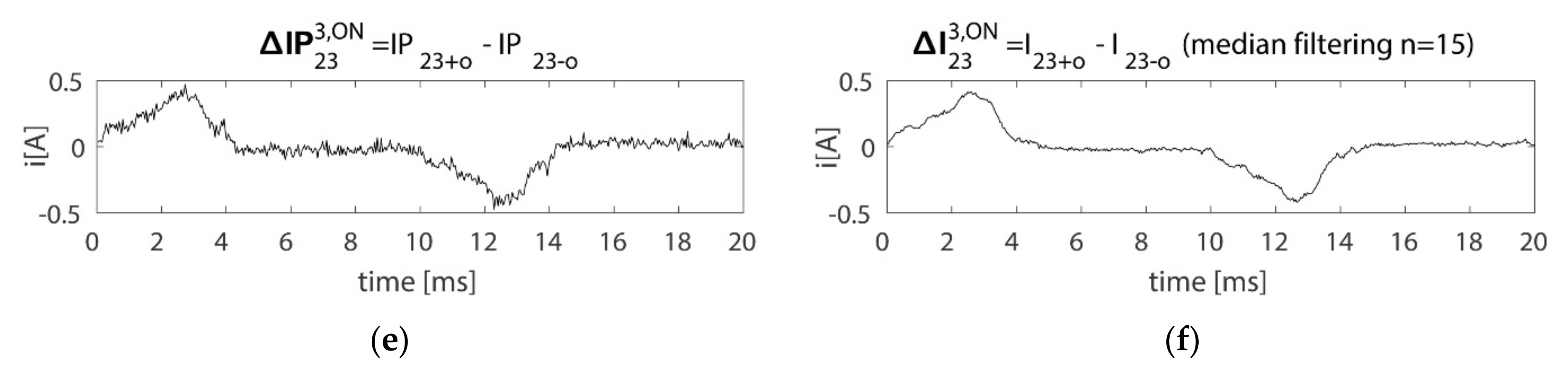
Figure 6 shows vectors   I P k a , s   calculated for the signal from Figure 5a and I k a , s for the signal from Figure 5b.
Similarly to [27], the proposed method allows for identifying the specific appliances with all possible combinations of devices working in the background. Recording only the single state change of each appliance is required for this purpose. During the event from Figure 4 and 
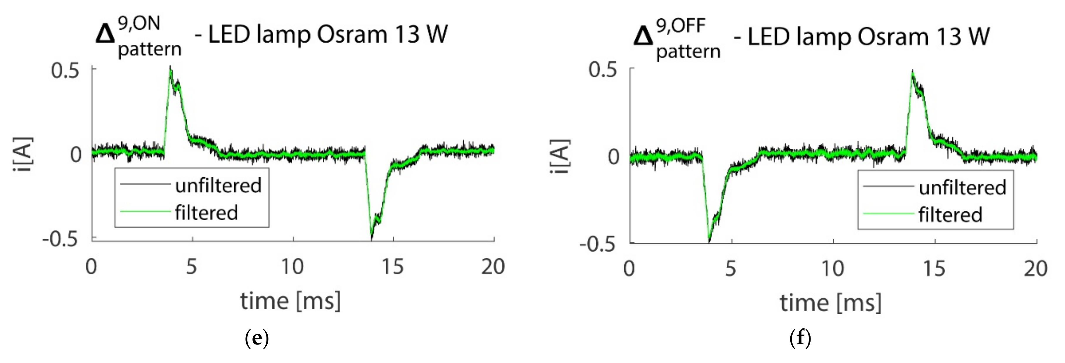
Figure 5, the transient state lasts for less than one period of the voltage signal, which is enough in our case. Vectors of samples’ changes Δ I p a t t e r n a , s obtained when turning the selected appliances on are presented in Figure 7. Black patterns extracted from the filtered array I are visible with original, green vectors from the I P array in the background. Similar patterns were observed while turning the devices on: LED Philips 13 W—Figure 7c and LED Osram 13 W—Figure 7e.
Filtering allowed for highlighting the signal components’ characteristics.

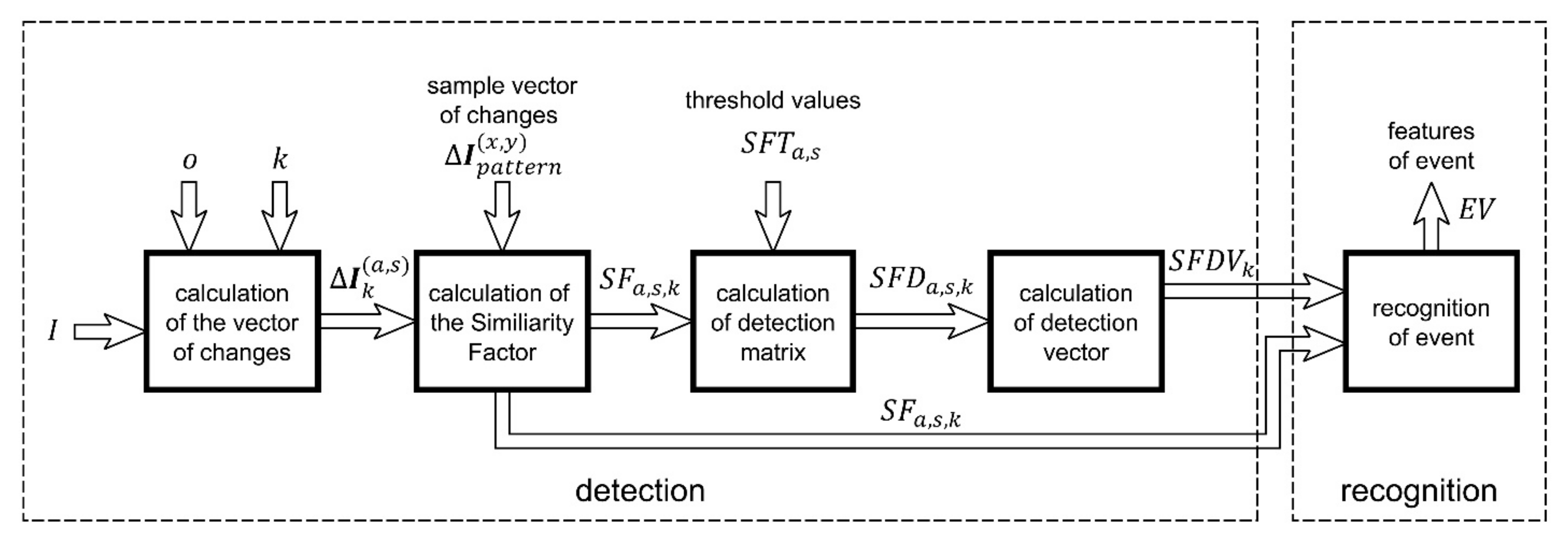
3.3. Event Detection and Appliance Identification

The event detection in the proposed method is carried out independently for each appliance. Subsequent steps taken during each period are presented in 
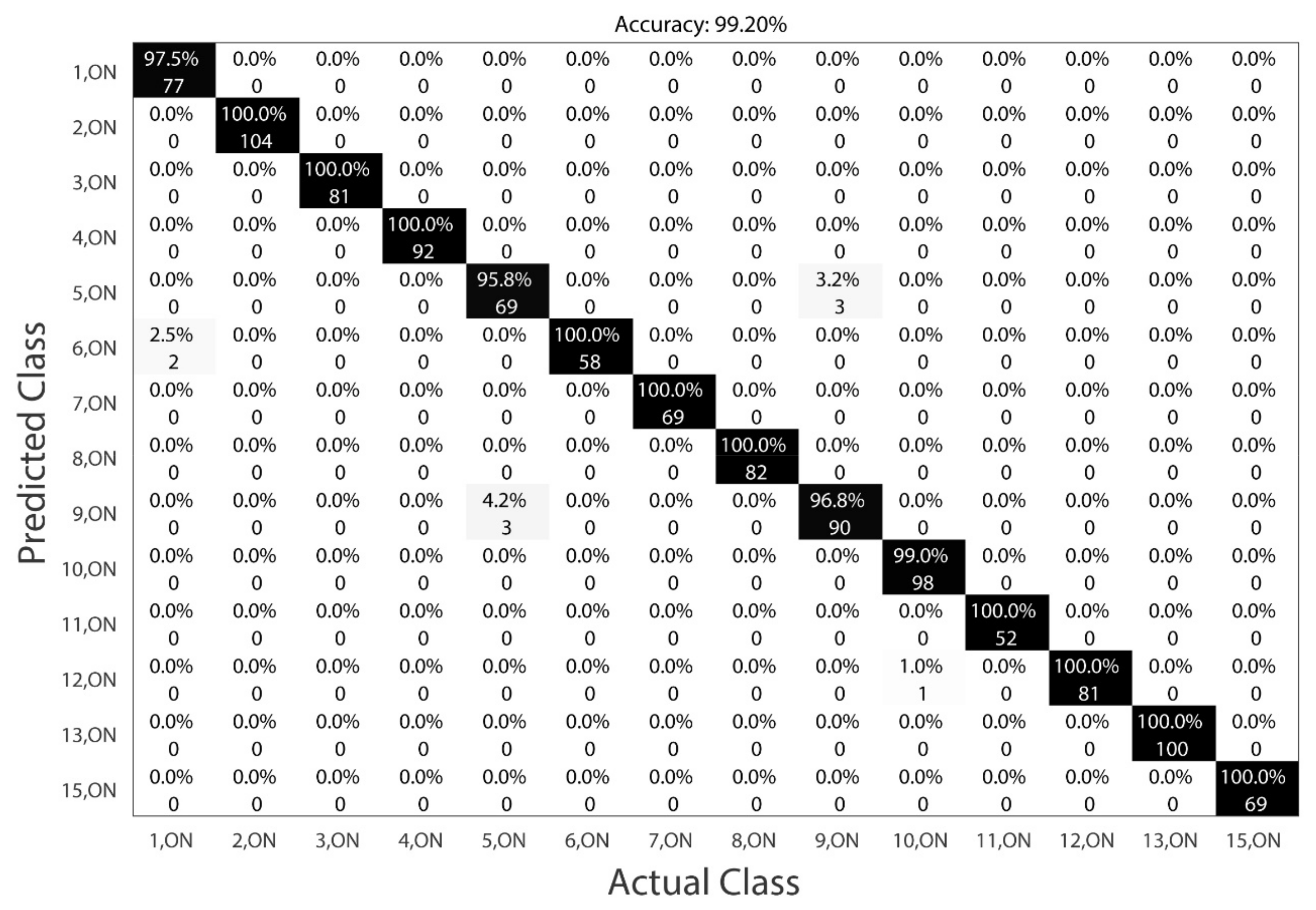
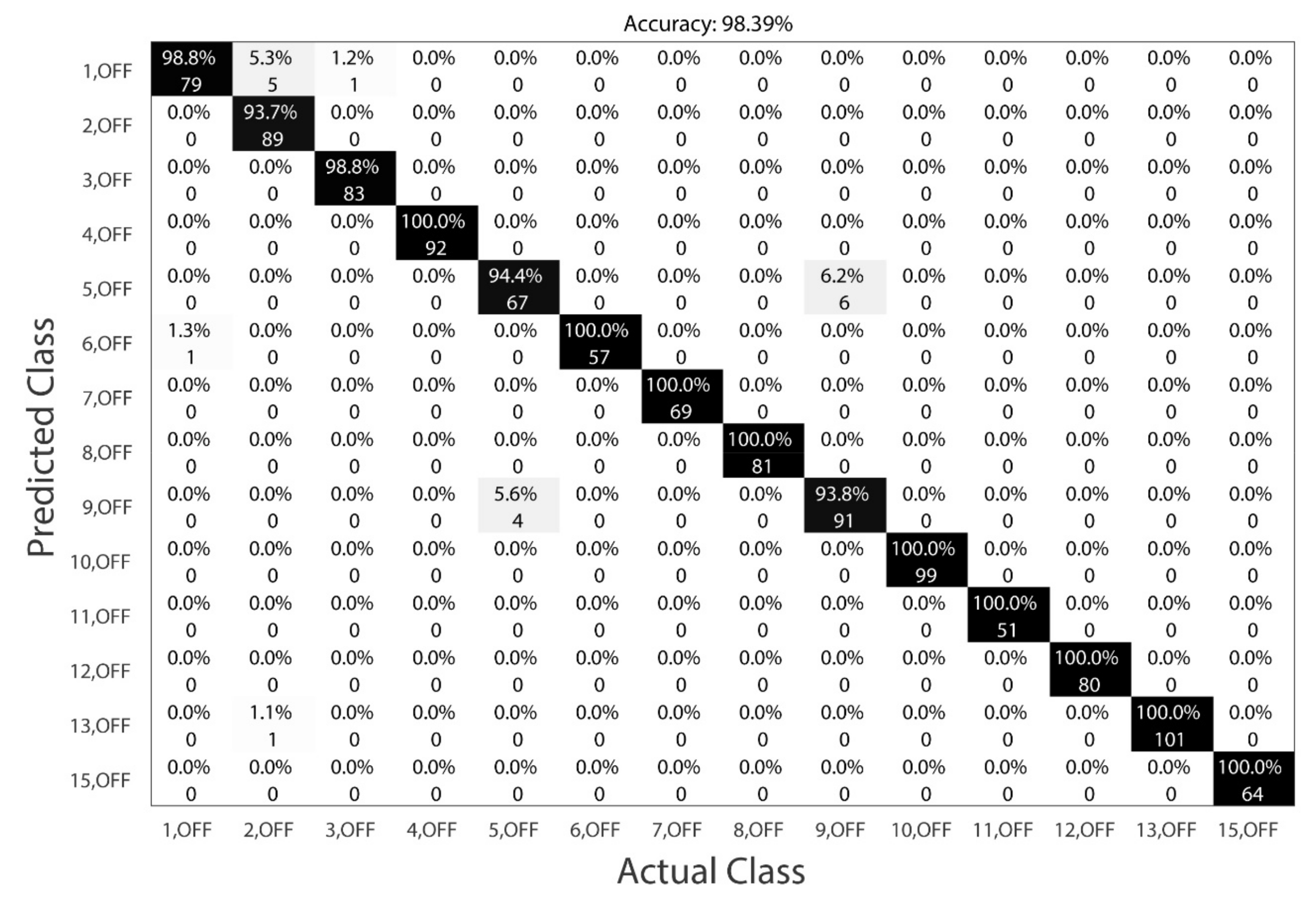
Figure 8. Selected 14 devices can be in 2 states (ON or OFF), which gives 28 categories to identify.
Table 2 shows the most useful values of o 15 , 30 , 60 , 120 for specific subsets of devices. To detect the appliance change, the differences between vectors Δ I k a , s (2) are calculated to determine the similarity S F a , s , k 0 , (5) between the analyzed pattern Δ I p a t t e r n a , s and all patterns in the dictionary. The minimum Euclidean distance d E Δ I k a , s , Δ I p a t t e r n a , s identifies the event { a , s }, i.e., device a changing state into s . The average absolute value σ (4) of Δ I p a t t e r n a , s normalizes values of S F in (5) for different devices. Calculation of the Euclidean metric facilitates visualization of the values of SF. When S F a , s , k exceeds the threshold value S F T a , s for the device a and state s , it means that in the k-th period, the event a , s occurs. The thresholds are experimentally set to either 2 or 5, the former being enough for devices with power below 50 W.
σ = 1 M · i = 1 M x i = 1 M · i = 1 M Δ I p a t t e r n a , s i
S F a , s , k = σ d E Δ I k a , s , Δ I p a t t e r n a , s = σ Δ I k a , s Δ I p a t t e r n a , s ,     k   N     k   o + 1 , K o
To indicate the potential time instants of events in the system, the detection array S F D a , s , k is calculated:
S F D a , s , k = 1 ,         S F a , s , k S F T a , s 0 ,         S F a , s , k < S F T a , s .
Summing columns of S F D a , s , k produces the detection vector S F D V k , indicating how many appliances potentially changed state in the k-th period.
S F D V k = a = 1 15 s = O N , O F F S F D a , s , k ,   w h e r e   k     < 1 , K > .
Potential errors of the algorithm are due to the similar patterns Δ I p a t t e r n a , s for different appliances. For instance, events a,s = {5,ON} (turning the LED Philips 13 W on) and a,s = {9,ON} (turning the LED Osram 13 W on) are difficult to distinguish. In particular, it is possible that for more than one device, the value of S F a , s , k exceeds the threshold value S F T a , s . In such a situation, the device with the highest value of S F a , s , k is considered to be the one that changed its state.
To limit false-positive detections, it was assumed that two subsequent events have to be separated by at least 0.2 s. Secondly, the duration of the event (number of consecutive periods during which the value of S F a , s , k is greater than threshold value S F T a , s ) must last longer than half of the value o . That eliminates false detections resulting from short-term changes in the signal during which the vector of changes Δ I k a , s is similar to any pattern Δ I p a t t e r n a , s .

4. Experimental Results

The proposed method can be used to detect and recognize states of single appliances. Evaluated events are presented in Table 4 with the number of the turn on and off events meeting this criterion for each device (corresponding to Table 1).

4.1. Appliance Recognition Accuracy with Known Time Instant of the State Change

This section presents the scenario when the time instant of the event is already known. This case was considered to make comparisons with results obtained for data sets such as REDD [28], PLAID [30,31,32,33,34] or WHITED [30,32], where the event detection was not considered. This allows for verifying just the event classification accuracy (assuming the detection is already complete). To evaluate the usability of transforming the signal into the array form and median filtering of each row, the classification of events was applied, exploiting the dictionary method, i.e., by finding the smallest Euclidean distance between the changes vector Δ I e v   of the analyzed example and all feature vectors Δ I p a t t e r n a , s in the data set, containing 28 entries, as each category is represented by only one “ideal” example. The testing set consisted of 2252 events belonging to 28 categories.
In the laboratory conditions (where each socket current is individually measured), the actual configuration of appliances connected to the network is always known. It was then possible to determine in which period the particular event should be detected. The classified changes vectors are defined as follows:
Δ I e v = I k e v + o I k e v o   ,   f o r   k   N   e v     1 , 2252
where k e v is the period number, in which the e v -th event (change of the state s by the appliance a) occurred. Values of o were predefined for periods k e v + o   and k e v o   , where the device was already in the steady state. Pattern vectors Δ I p a t t e r n a , s   were selected to represent events where only the device a was active. Though the base fs = 250 kHz, lower frequencies were used to check if accurate event classification is possible for them. Comparison of the identification accuracy for different sampling frequencies is shown in Table 5. The green color indicates the best result for each frequency.
The detection accuracy is proportional to fs, which has a significant impact on the system accuracy. Application of the median filter allowed for increasing the accuracy by an average of 5%. The preferred values of its length are between 9 and 25 (this selection is of secondary significance, because most results around optimal values are similar). The highest accuracy (ratio of the correctly identified events) was 98.80%, which was achieved for fs = 250 kHz and 23rd order median filter.
Detailed results are presented using the confusion matrix, where the main diagonal represents the correct classifications (True Positive—TP) and the other values represent misclassifications [22,46]. Figure 9 and Figure 10 show confusion matrices for particular events in the optimal combination of the filter’s length and sampling frequency (switching devices on and off, respectively). The risk of the identification error decreases as the device power increases. This is a result of the increasing Euclidean distance between the device patterns (see (5)). Overall accuracies were calculated separately only for switching-on events (Figure 9) and switching-off events (Figure 10).
Identification errors for the tv set (EA 2, OFF) are caused by the fact that this device does not have the constant duration of the transient state, leading to varying values of vectors Δ I e v calculated from (8). In this case, the proposed method does not work. For appliances with constant duration of the transient state, for 19 classes, there is 100% accuracy.
The highest number of errors (50% of all misclassifications) is encountered for the LED Philips 13 W lamp (categories 5,ON and 5,OFF) and LED Osram 13 W lamp (categories 9,ON and 9,OFF). Both have very similar signatures. Figure 11 shows changes’ vectors for events 5,ON and 9,ON.
Based on the results presented in Figure 9 and Figure 10, metrics common in NILM, such as recall, precision and F-score [46,47] were calculated—see Table 6. The lowest F-score (0.9306) was obtained for category {5,OFF} (switching off LED Philips 13 W lamp). Four events of this class was classified to another class (False Negative—FN) and six events of another class was incorrectly classified to category {5,OFF} (False Positive—FP). All false positives for category {5,OFF} were events of category {9,OFF} and vice versa.
The macro-averaged F-score was 0.9874, which is a result comparable to the most accurate known methods with macro averaged F-scores of 0.9939 in [34] and 0.9777 in [31]. Both referenced results were achieved on the PLAID data set (only up to two devices operating at the same time). Most of the existing methods identify the general type of devices rather than a specific appliance. This requires a significant amount of training data, e.g., using a 10-fold cross-validation model that is trained on 90% of the data and tested on the remaining 10% [31]. The classifier used in our study requires only one observation of each state change of a new device added to the system, but it identifies this specific appliance.

4.2. Event Detection Accuracy in the Real-World Conditions

In the practical application (end-user’s apartment), the information about the time of the event is not known. Therefore, the proper prior event detection (see Section 3.3) must be completed. Metrics commonly used to evaluate classifiers in NILM were used to evaluate the performance of the proposed detection method—identification accuracy, recall, precision, and F-score [46,47]. The obtained detection results are presented in Table 7 (switching on) and Table 8 (switching off). Out of all 2252 events, 2225 were detected correctly (TP), and the achieved detection accuracy was 98.8%. In total, 37 detections were false alarms (FP), and 27 events were incorrectly undetected (FN). For the majority of appliances, the detection rate was high, including the power efficient ones (such as LED bulbs). The latter are especially difficult to detect with multiple devices operating in the background (as Table 9 shows). The mostly omitted events include turning the tv set off (due to the already explained varying duration of the transient state). The relatively high number of false detections (i.e., 13) for switching the fan off (EA ID 6, OFF) is caused by the same effect.

4.3. Appliance Recognition for the Detected Events

This section covers accuracy analysis of the classification module. All 2225 correctly detected events are assigned to particular categories. Figure 12 presents the confusion matrix for all ON events (the number of classified events for each class is equal to TP in Table 7). Figure 13 contains the confusion matrix for the respective OFF events (the number of classified events for each class is equal to TP in Table 8). The overall accuracies above the confusion matrices were calculated separately for switching-on (Figure 12) and switching-off events (Figure 13). The analyzed data were collected with fs = 250 kHz (without subsampling). The IP array was processed by the median filter with the length of 15. Classification was completed using the nearest-neighbor approach (see Section 4.1).
The average appliance identification accuracy was 98.97% (99.02% for turning the devices on and 98.90% for turning them off). The most common errors included identifying the state {5,ON} as {9,ON} (eight errors) and the state {5,OFF} as {9,OFF} (10 errors). These are difficult to distinguish (both appliances are lamps with LED bulbs: Philips 13 W and Osram 13 W, with similar signature—Figure 11). The obtained accuracy depends on the prior ability to correctly detect the event, so the overall performance (considering detection errors) was 97.78%. Please note that only one dictionary entry for each recognized class was used.
Compared to Section 4.1, there were more classification errors, even though more events were identified in Section 4.1 (2252 vs. 2225 here). This is due to the fact that in the previous experiment, the time of state change of the appliances was precisely known. The identified vectors of changes were determined more accurately than when the time of state change is determined by the event detection algorithm.
For 23 categories, the accuracy was 100% (even if there are multiple appliances operating in the background—see Table 7, Table 8 and Table 9). The operation of many devices at the same time is the typical work regime of electrical appliances in the household. The obtained results prove that the calculation of current signatures allows for the accurate identification of appliances’ states.

5. Conclusions

A high accuracy of detection and recognition of appliances’ state changes was achieved with the knowledge of only one observation of a particular appliance. These were used to calculate the appliances’ signatures. A dictionary method was used for classification. Unlike the methods described in other papers, the proposed method identifies the particular appliance and not just its general type. For the purpose of this research, a data set containing 2252 events was created. At least five devices were operating during most of the analyzed events.
The presented event detection algorithm achieved an F-score of 0.986 and for specific appliance identification, the macro-averaged F-score was 0.9874 for known events. The flawless performance was obtained for 23 out of 28 identified categories. The algorithm was able to distinguish appliances with similar signatures. The method fills the gap in knowledge by being resilient to the number and configuration of appliances working in the background.
A novel approach to analyze voltage and current signals in the time domain was proposed. The periodicity of the network voltage was used to construct the array-like representation of the current samples. It allows for filtering each row separately to isolate features of each device. Applying the proposed signal processing and filtering method allows for increasing the accuracy by an average of 5%. The median filter with the length between 13 and 25 samples was the most useful here. Although even fs = 1 kHz provides satisfactory results, an increase in accuracy was observed for higher frequencies. Median filtering allows also for a reduction in the sampling rate without a decrease in the identification accuracy (accuracy 97.91% for fs = 2.5 kHz with 15th order filter compared to 93.96% fs = 250 kHz without filtering). This signal processing method can be beneficial when applied to other NILM methods: especially methods based on the V-I trajectory analysis, which so far have been mainly tested on data sets with a low number of devices operating in the background
The disadvantage of the method is that it does not correctly process appliances whose transient state duration is varying. Further research will cover verification on public data sets and comparison against other algorithms.
This novel approach can be widely used being a part of smart meters in a smart grid, allowing for the decrease in end-user energy consumption and cost.

Author Contributions

Conceptualization, R.K. and K.D.; methodology, K.D.; software, K.D.; validation, R.K., A.W. and R.Ł.; formal analysis, R.K.; investigation, K.D. and A.W.; resources, A.W. and K.D.; data curation, K.D.; writing—original draft preparation, K.D.; writing—review and editing, R.Ł. and P.B.; visualization, R.Ł.; supervision, P.B.; project administration, P.B.; funding acquisition, R.K. and R.Ł. All authors have read and agreed to the published version of the manuscript.

Funding

The research was funded by the POB Energy of Warsaw University of Technology within the Excellence Initiative: Research University (IDUB) program, agreement 1820/343/Z01/POB7/2021.

Institutional Review Board Statement

Not applicable.

Informed Consent Statement

Not applicable.

Data Availability Statement

The data presented in this study are available on request from the corresponding author.

Conflicts of Interest

The authors declare no conflict of interest.

References

  1. Hart, G.W. Nonintrusive Appliance Load Monitoring. Proc. IEEE 1992, 80, 1870–1891. [Google Scholar] [CrossRef]
  2. Wójcik, A.; Łukaszewski, R.; Kowalik, R.; Winiecki, W. Nonintrusive Appliance Load Monitoring: An Overview, Laboratory Test Results and Research Directions. Sensors 2019, 19, 3621. [Google Scholar] [CrossRef] [PubMed] [Green Version]
  3. Carrie Armel, K.; Gupta, A.; Shrimali, G.; Albert, A. Is Disaggregation the Holy Grail of Energy Efficiency? The Case of Electricity. Energy Policy 2013, 52, 213–234. [Google Scholar] [CrossRef] [Green Version]
  4. De Souza, W.A.; Garcia, F.D.; Marafão, F.P.; Da Silva, L.C.P.; Simões, M.G. Load Disaggregation Using Microscopic Power Features and Pattern Recognition. Energies 2019, 12, 2641. [Google Scholar] [CrossRef] [Green Version]
  5. Zeifman, M.; Roth, K. Nonintrusive Appliance Load Monitoring: Review and Outlook. IEEE Trans. Consum. Electron. 2011, 57, 76–84. [Google Scholar] [CrossRef]
  6. Huber, P.; Calatroni, A.; Rumsch, A.; Paice, A. Review on Deep Neural Networks Applied to Low-Frequency NILM. Energies 2021, 14, 2390. [Google Scholar] [CrossRef]
  7. Moreno Jaramillo, A.F.; Laverty, D.M.; Morrow, D.J.; Martinez del Rincon, J.; Foley, A.M. Load Modelling and Non-Intrusive Load Monitoring to Integrate Distributed Energy Resources in Low and Medium Voltage Networks. Renew. Energy 2021, 179, 445–466. [Google Scholar] [CrossRef]
  8. Tabatabaei, S.M.; Dick, S.; Xu, W. Toward Non-Intrusive Load Monitoring via Multi-Label Classification. IEEE Trans. Smart Grid 2017, 8, 26–40. [Google Scholar] [CrossRef]
  9. Gupta, S.; Reynolds, M.S.; Patel, S.N. ElectriSense: Single-Point Sensing Using EMI for Electrical Event Detection and Classification in the Home. In Proceedings of the 12th ACM International Conference on Ubiquitous Computing, New York, NY, USA, 26 September 2010; pp. 139–148. [Google Scholar]
  10. Liu, B.; Luan, W.; Yu, Y. Dynamic Time Warping Based Non-Intrusive Load Transient Identification. Appl. Energy 2017, 195, 634–645. [Google Scholar] [CrossRef]
  11. Zhao, B.; Stankovic, L.; Stankovic, V. On a Training-Less Solution for Non-Intrusive Appliance Load Monitoring Using Graph Signal Processing. IEEE Access 2016, 4, 1784–1799. [Google Scholar] [CrossRef] [Green Version]
  12. Li, D.; Dick, S. Whole-House Non-Intrusive Appliance Load Monitoring via Multi-Label Classification. In Proceedings of the 2016 International Joint Conference on Neural Networks (IJCNN), Vancouver, BC, Canada, 24–29 July 2016; pp. 2749–2755. [Google Scholar] [CrossRef]
  13. Henao, N.; Agbossou, K.; Kelouwani, S.; Dube, Y.; Fournier, M. Approach in Nonintrusive Type i Load Monitoring Using Subtractive Clustering. IEEE Trans. Smart Grid 2017, 8, 812–821. [Google Scholar] [CrossRef]
  14. Kong, W.; Dong, Z.; Xu, Y.; Hill, D. An Enhanced Bootstrap Filtering Method for Non-Intrusive Load Monitoring. In Proceedings of the 2016 IEEE Power and Energy Society General Meeting (PESGM), Boston, MA, USA, 17–21 July 2016; pp. 4–8. [Google Scholar] [CrossRef]
  15. Jia, Z.; Yang, L.; Zhang, Z.; Liu, H.; Kong, F. Sequence to Point Learning Based on Bidirectional Dilated Residual Network for Non-Intrusive Load Monitoring. Int. J. Electr. Power Energy Syst. 2021, 129, 106837. [Google Scholar] [CrossRef]
  16. Jiang, J.; Kong, Q.; Plumbley, M.; Gilbert, N. Deep Learning Based Energy Disaggregation and On/Off Detection of Household Appliances. ACM Trans. Knowl. Discov. Data 2019, 15, 1–21. [Google Scholar] [CrossRef]
  17. Çavdar, I.H.; Faryad, V. New Design of a Supervised Energy Disaggregation Model Based on the Deep Neural Network for a Smart Grid. Energies 2019, 12, 1217. [Google Scholar] [CrossRef] [Green Version]
  18. Wu, Z.; Wang, C.; Zhang, H.; Peng, W.; Liu, W. A Time-Efficient Factorial Hidden Semi-Markov Model for Non-Intrusive Load Monitoring. Electr. Power Syst. Res. 2021, 199, 107372. [Google Scholar] [CrossRef]
  19. Wu, Z.; Wang, C.; Peng, W.; Liu, W.; Zhang, H. Non-Intrusive Load Monitoring Using Factorial Hidden Markov Model Based on Adaptive Density Peak Clustering. Energy Build. 2021, 244, 111025. [Google Scholar] [CrossRef]
  20. Meehan, P.; McArdle, C.; Daniels, S. An Efficient, Scalable Time-Frequency Method for Tracking Energy Usage of Domestic Appliances Using a Two-Step Classification Algorithm. Energies 2014, 7, 7041–7066. [Google Scholar] [CrossRef] [Green Version]
  21. Guo, L.; Wang, S.; Chen, H.; Shi, Q. A Load Identification Method Based on Active Deep Learning and Discrete Wavelet Transform. IEEE Access 2020, 8, 113932–113942. [Google Scholar] [CrossRef]
  22. Wójcik, A.; Bilski, P.; Łukaszewski, R.; Dowalla, K.; Kowalik, R. Identification of the State of Electrical Appliances with the Use of a Pulse Signal Generator. Energies 2021, 14, 673. [Google Scholar] [CrossRef]
  23. Agyeman, K.A.; Han, S.; Han, S. Real-Time Recognition Non-Intrusive Electrical Appliance Monitoring Algorithm for a Residential Building Energy Management System. Energies 2015, 8, 9029–9048. [Google Scholar] [CrossRef]
  24. Bouhouras, A.S.; Gkaidatzis, P.A.; Panagiotou, E.; Poulakis, N.; Christoforidis, G.C. A NILM Algorithm with Enhanced Disaggregation Scheme under Harmonic Current Vectors. Energy Build. 2019, 183, 392–407. [Google Scholar] [CrossRef]
  25. Le, T.T.H.; Kang, H.; Kim, H. Household Appliance Classification Using Lower Odd-Numbered Harmonics and the Bagging Decision Tree. IEEE Access 2020, 8, 55937–55952. [Google Scholar] [CrossRef]
  26. Lam, H.Y.; Fung, G.S.K.; Lee, W.K. A Novel Method to Construct Taxonomy Electrical Appliances Based on Load Signatures. IEEE Trans. Consum. Electron. 2007, 53, 653–660. [Google Scholar] [CrossRef] [Green Version]
  27. Hassan, T.; Javed, F.; Arshad, N. An Empirical Investigation of V-I Trajectory Based Load Signatures for Non-Intrusive Load Monitoring. IEEE Trans. Smart Grid 2014, 5, 870–878. [Google Scholar] [CrossRef] [Green Version]
  28. Wang, A.L.; Chen, B.X.; Wang, C.G.; Hua, D.D. Non-Intrusive Load Monitoring Algorithm Based on Features of V–I Trajectory. Electr. Power Syst. Res. 2018, 157, 134–144. [Google Scholar] [CrossRef]
  29. Du, L.; He, D.; Harley, R.G.; Habetler, T.G. Electric Load Classification by Binary Voltage-Current Trajectory Mapping. IEEE Trans. Smart Grid 2016, 7, 358–365. [Google Scholar] [CrossRef]
  30. Liu, Y.; Wang, X.; You, W. Non-Intrusive Load Monitoring by Voltage–Current Trajectory Enabled Transfer Learning. IEEE Trans. Smart Grid 2019, 10, 5609–5619. [Google Scholar] [CrossRef]
  31. Faustine, A.; Pereira, L.; Klemenjak, C. Adaptive Weighted Recurrence Graphs for Appliance Recognition in Non-Intrusive Load Monitoring. IEEE Trans. Smart Grid 2021, 12, 398–406. [Google Scholar] [CrossRef]
  32. Faustine, A.; Pereira, L. Improved Appliance Classification in Non-Intrusive Load Monitoring Usingweighted Recurrence Graph and Convolutional Neural Networks. Energies 2020, 13, 3374. [Google Scholar] [CrossRef]
  33. Faustine, A.; Pereira, L. Multi-Label Learning for Appliance Recognition in NILM Using Fryze-Current Decomposition and Convolutional Neural Network. Energies 2020, 13, 4154. [Google Scholar] [CrossRef]
  34. Li, K.; Yin, B.; Du, Z.; Sun, Y. A Nonintrusive Load Identification Model Based on Time-Frequency Features Fusion. IEEE Access 2021, 9, 1376–1387. [Google Scholar] [CrossRef]
  35. Iqbal, H.K.; Malik, F.H.; Muhammad, A.; Qureshi, M.A.; Abbasi, M.N.; Chishti, A.R. A Critical Review of State-of-the-Art Non-Intrusive Load Monitoring Datasets. Electr. Power Syst. Res. 2021, 192, 106921. [Google Scholar] [CrossRef]
  36. Held, P.; Weibhaar, D.; Abdeslam, D.O.; Benyoucef, D. Generation of New Simulation Scenarios for NILM Based on Real Data Sets Using High-Resolution Current Waveforms. In Proceedings of the IECON 2019-45th Annual Conference of the IEEE Industrial Electronics Society, Lisbon, Portugal, 14–17 October 2019; pp. 5319–5324. [Google Scholar] [CrossRef]
  37. Klemenjak, C.; Makonin, S.; Elmenreich, W. Investigating the Performance Gap between Testing on Real and Denoised Aggregates in Non-Intrusive Load Monitoring. Energy Inform. 2021, 4, 3. [Google Scholar] [CrossRef]
  38. Wu, Q.; Wang, F. Concatenate Convolutional Neural Networks for Non-Intrusive Load Monitoring across Complex Background. Energies 2019, 12, 1572. [Google Scholar] [CrossRef] [Green Version]
  39. Egarter, D.; Bhuvana, V.P.; Elmenreich, W. PALDi: Online Load Disaggregation via Particle Filtering. IEEE Trans. Instrum. Meas. 2015, 64, 467–477. [Google Scholar] [CrossRef]
  40. Kamyshev, I.; Kriukov, D.; Gryazina, E. COLD: Concurrent Loads Disaggregator for Non-Intrusive Load Monitoring. arXiv 2021, arXiv:2106.02352. [Google Scholar]
  41. Held, P.; Mauch, S.; Saleh, A.; Abdeslam, D.O.; Benyoucef, D. Frequency Invariant Transformation of Periodic Signals (FIT-PS) for Classification in NILM. IEEE Trans. Smart Grid 2018, 10, 5556–5563. [Google Scholar] [CrossRef]
  42. Liu, Y.; Wang, X.; Zhao, L.; Liu, Y. Admittance-Based Load Signature Construction for Non-Intrusive Appliance Load Monitoring. Energy Build. 2018, 171, 209–219. [Google Scholar] [CrossRef]
  43. Chen, K.L.; Chang, H.H.; Chen, N. A New Transient Feature Extraction Method of Power Signatures for Nonintrusive Load Monitoring Systems. In Proceedings of the 2013 IEEE International Workshop on Applied Measurements for Power Systems (AMPS), Aachen, Germany, 25–27 September 2013; pp. 79–84. [Google Scholar]
  44. Chung, J.; Gillis, J.M.; Morsi, W.G. Non-Intrusive Load Monitoring Using Wavelet Design and Co-Testing of Machine Learning Classifiers. In Proceedings of the 2016 IEEE Electrical Power and Energy Conference (EPEC), Ottawa, ON, Canada, 12–14 October 2016; Volume 8, pp. 2648–2655. [Google Scholar]
  45. Oziemblewski, K.; Opala, K. Static Stability of Electric Al Power Engineering Systems: Power Swing. Energetyka 2015, 4, 4–10. [Google Scholar]
  46. Kohavi, R.; Provost, F. Glossary of Terms. Mach. Learn. 1998, 30, 271–274. [Google Scholar] [CrossRef]
  47. Makonin, S.; Popowich, F. Nonintrusive Load Monitoring (NILM) Performance evaluation—A Unified Approach for Accuracy Reporting. Energy Effic. 2015, 8, 809–814. [Google Scholar] [CrossRef]
Figure 1. General architecture of a non-intrusive load monitoring system.
Energies 15 03325 g001
Figure 2. Scheme of measuring system.
Energies 15 03325 g002
Figure 3. Subsequent steps are required to extract the vector of changes Δ I k a , s .
Energies 15 03325 g003
Figure 4. An example of a recorded current signal and filtered voltage u f (a). During recording, a wall lamp with 4 LED lamps was turned on (b, period no. 23).
Energies 15 03325 g004
Figure 5. An example of changes in a pseudo-periodic signal caused by the inclusion of an additional appliance. (a,b) represent the same event. The signal on (a) array I P was not filtered, the signal on (b) array I was filtered by the 15th order median filter.
Energies 15 03325 g005
Figure 6. Determination of changes in the current signal—determination of the vector of changes Δ I P k a , s , on the unfiltered signal (a,c,e) and the change vector Δ I k a , s on the filtered signal median of the 15th order (b,d,f) for k = 23, a = 3, s = ON, o = 15 . (Before the analyzed event took place, another 7 EAs was already on, working in the background).
Energies 15 03325 g006aEnergies 15 03325 g006b
Figure 7. Comparison between sample vectors Δ I p a t t e r n a , s for selected appliances. (a) switch ON of the light bulb—AE no. 1, (b) switch ON of the TV—AE no. 2, (c) switch ON of the led lamp Philips 13W– AE no. 5, (d) switch ON of the fan—AE no. 6, (e) switch ON of the LED lamp OSRAM—AE no. 9, (f) switch OFF of the LED lamp OSRAM—AE no. 9.
Energies 15 03325 g007aEnergies 15 03325 g007b
Figure 8. Current signature calculation algorithm.
Energies 15 03325 g008
Figure 9. Confusion matrix for recognizing switch-on events of tested appliances using the dictionary method.
Energies 15 03325 g009
Figure 10. Confusion matrix for recognizing switch-off events of tested appliances using the dictionary method.
Energies 15 03325 g010
Figure 11. Comparison of sample vectors of changes for appliance of categories 5,ON and 9,ON.
Energies 15 03325 g011
Figure 12. Confusion matrix for the recognition of switching-on events of the tested appliances using the proposed method. Only events detected by the detection algorithm were the subject of recognition.
Energies 15 03325 g012
Figure 13. Confusion matrix for the recognition of switching-off events of the tested appliances using the proposed method. Only events detected by the detection algorithm were the subject of recognition.
Energies 15 03325 g013
Table 1. Characteristics of the electrical appliances (EAs) selected for experiments.
aMeasured ApplianceNumber of EventsaMeasured ApplianceNumber of Events
8Vacuum cleaner Zelmer163
1Light bulb 1769Lamp LED Osram 13 W192
2TV LED Samsung22010LED Osram 17 W203
34x LED Lightec Eco 5 W16711Electric Kettle104
4Slow juicer18512Hair dryer162
5LED Philips lamp 13W14613Fluorescent lamp207
6Fan11814Fridge0
7Air heater 1100 W14015Microwave153
Table 2. Values of o and S F T a , s for events of turning the appliances on.
as o S F T a , s as o S F T a , s
1ON1558ON305
2ON6059ON152
3ON15210ON152
4ON30511ON155
5ON15212ON155
6ON15513ON302
7ON30515ON1205
Table 3. Values of o and S F T a , s for events of turning the appliances off.
as o S F T a , s as o S F T a , s
1OFF1558OFF305
2OFF6029OFF152
3OFF15210OFF152
4OFF15511OFF155
5OFF15212OFF305
6OFF30213OFF152
7OFF30515OFF305
Table 4. Number of events related to the switch off or on events for selected appliances.
App No.1234567891011121315Overall
ON7910481927258698293995281100691131
OFF809584927157698197995180101641121
overall1591991651841431151381631901981031612011332252
Table 5. Event identification accuracy using the dictionary method.
Filter OrderSampling Frequency [kHz]
0.100.150.200.250.5012.55102550250
Accuracy [%]
136.2868.2570.1283.1784.7787.2692.4193.2193.8393.9694.0193.96
338.1471.4575.5385.6686.7289.2193.3493.5694.3694.4594.3294.36
539.0373.0076.7886.8686.6890.5495.8396.1496.7196.9896.8597.02
741.5275.3679.2289.3990.4593.6997.6597.8798.5898.6798.6798.62
942.0575.6778.2490.0190.5993.8797.6598.0098.4998.6298.6298.58
1141.5676.2479.9390.1490.7694.4997.6597.6098.5398.6298.5898.58
1340.8576.1578.4690.6391.2194.2797.8297.7498.6298.6798.5898.58
1541.1278.6480.2890.0590.7294.8597.9197.5198.6298.7198.6298.67
1743.7478.9180.5190.4191.4795.3497.7497.6998.6298.7698.6298.62
1944.1478.6980.2490.6791.3994.7697.8797.7498.6298.6298.6298.67
2142.9878.8280.6091.0391.6594.8597.6997.7898.5898.7698.6798.76
2342.1077.7180.1190.7690.9994.5897.7897.8298.7198.7198.7698.80
2543.3877.2680.2089.9291.1294.1497.5697.8798.6298.6798.7698.80
5038.9472.7475.2288.5488.9091.3995.5696.5896.9497.1697.1197.07
10040.2869.0974.7886.1086.1089.0392.9094.7695.2594.9495.0395.03
Table 6. Appliance recognition results with known time instant of the state change.
EA IDNumber of EventsTPFPFNRecallPrecisionF
1,ON797702100.0097.470.9872
2,ON1041011399.0297.120.9806
3,ON818100100.00100.001.0000
4,ON929200100.00100.001.0000
5,ON72693395.8395.830.9583
6,ON585800100.00100.001.0000
7,ON696900100.00100.001.0000
8,ON828200100.00100.001.0000
9,ON93903396.7796.770.9677
10,ON999801100.0098.990.9949
11,ON525200100.00100.001.0000
12,ON818100100.00100.001.0000
13,ON100981298.9998.000.9849
15,ON69691098.57100.000.9928
1,OFF80796192.9498.750.9576
2,OFF958906100.0093.680.9674
3,OFF848301100.0098.810.9940
4,OFF929200100.00100.001.0000
5,OFF71676491.7894.370.9306
6,OFF575700100.00100.001.0000
7,OFF696900100.00100.001.0000
8,OFF81811098.78100.000.9939
9,OFF97914695.7993.810.9479
10,OFF99991099.00100.000.9950
11,OFF515100100.00100.001.0000
12,OFF808000100.00100.001.0000
13,OFF1011011099.02100.000.9951
15,OFF646400100.00100.001.0000
average
(F-macro)
0.9874
Table 7. Event detection results (switching on).
EA IDNumber of EventsTPFPFNRecallPrecisionF
ALL22892225372798.8098.360.986
1-15,ON113511234899.2999.650.995
1,ON797900100.00100.001.000
2,ON1041011397.1299.020.981
3,ON818100100.00100.001.000
4,ON929200100.00100.001.000
5,ON727200100.00100.001.000
6,ON58570198.28100.000.991
7,ON696900100.00100.001.000
8,ON828200100.00100.001.000
9,ON93920198.92100.000.995
10,ON99981198.9998.990.990
11,ON525200100.00100.001.000
12,ON818100100.00100.001.000
13,ON100981298.0098.990.985
15,ON696910100.0098.570.993
Table 8. Event detection results (switching off).
EA IDNumber of EventsTPFPFNRecallPrecisionF
1-15,OFF11541102331998.3197.090.977
1,OFF808020100.0097.560.988
2,OFF9581131485.2686.170.857
3,OFF84830198.81100.000.994
4,OFF929200100.00100.001.000
5,OFF71700198.59100.000.993
6,OFF5757130100.0081.430.898
7,OFF696910100.0098.570.993
8,OFF818110100.0098.780.994
9,OFF979700100.00100.001.000
10,OFF999910100.0099.000.995
11,OFF51501198.0498.040.980
12,OFF80790198.75100.000.994
13,OFF1011001199.0199.010.990
15,OFF646400100.00100.001.000
Table 9. Impact of the number of appliances working in the background on identification accuracy.
Number of Turned on Appliances at the Time of the Recognized EventNumber of EventsCorrectly RecognizedAccuracy [%]
0240240100
127327299.63
211711699.15
3181181100
427427399.64
537237099.46
632732398.78
722722096.92
813413097.01
9565496.43
101919100
114375
1211100
Publisher’s Note: MDPI stays neutral with regard to jurisdictional claims in published maps and institutional affiliations.

