Minimum Emissions Configuration of a Green Energy–Steel System: An Analytical Model

Abstract

The need to significantly reduce emissions from the steelmaking sector requires effective and ready-to-use technical solutions. With this aim, different decarbonization strategies have been investigated by both researchers and practitioners. To this concern, the most promising pathway is represented by the replacement of natural gas with pure hydrogen in the direct reduced iron (DRI) production process to feed an electric arc furnace (EAF). This solution allows to significantly reduce direct emissions of carbon dioxide from the DRI process but requires a significant amount of electricity to power electrolyzers adopted to produce hydrogen. The adoption of renewable electricity sources (green hydrogen) would reduce emissions by 95–100% compared to the blast furnace–basic oxygen furnace (BF–BOF) route. In this work, an analytical model for the identification of the minimum emission configuration of a green energy–steel system consisting of a secondary route supported by a DRI production process and a renewable energy conversion system is proposed. In the model, both technological features of the hydrogen steel plant and renewable energy production potential of the site where it is to be located are considered. Compared to previous studies, the novelty of this work consists of the joint modeling of a renewable energy system and a steel plant. This allows to optimize the overall system from an environmental point of view, considering the availability of green hydrogen as an inherent part of the model. Numerical experiments proved the effectiveness of the model proposed in evaluating the suitability of using green hydrogen in the steelmaking process. Depending on the characteristics of the site and the renewable energy conversion system adopted, decreases in emissions ranging from 60% to 91%, compared to the BF–BOF route, were observed for the green energy–steel system considered It was found that the environmental benefit of using hydrogen in the secondary route is strictly related to the national energy mix and to the electrolyzers’ technology. Depending on the reference context, it was found that there exists a maximum value of the emission factor from the national electricity grid below which is environmentally convenient to produce DRI by using only hydrogen. It was moreover found that the lower the electricity consumption of the electrolyzer, the higher the value assumed by the emission factor from the electricity grid, which makes the use of hydrogen convenient.

1. Introduction

Energy transition and industrial emissions abatement are key issues to tackle climate change and achieve the “net-zero” carbon emissions goal by 2050 [1]. To this concern, research efforts to investigate technological solutions enabling environmentally sustainable production are becoming mandatory. Some production sectors, due to their inherent difficulty to be converted into “carbon-free” sectors, are defined as “harder to abate”. One of these sectors is steelmaking; it results as extremely critical due to its strong energy and carbon dependency, generating the second-highest share of energy consumption among heavy industry sector and the highest share of emissions [2]. For the US steelmaking sector, it has been estimated that only 20% of the decarbonization pathways will meet the 2050 target [3]. The traditional blast furnace–basic oxygen furnace (BF–BOF) route relies indeed on the almost exclusive use of C-bearing materials (coal or coke) for both the energy and the chemical reduction needed along the steelmaking route, resulting in emissions and energy consumption of about 1.8 tCO_2eq/t crude steel [4], and 21 GJ/t crude steel [5], respectively. This process, still adopted in 73.2% of the worldwide plants in 2020 [6], is clearly not consistent with the current objectives, leading to the urgent need of a rethought. The identification of greener solutions for the steelmaking process is environmentally mandatory (emissions generated by this sector represented almost 7% of 2020 global emissions [7]) and is essential for the survival of most economic sectors. Steel is a feedstock for key economic sectors such as transport, construction, domestic appliances, electrical equipment, and machinery, and its demand is steadily increasing. On an annual basis, in 2021, a demand increase of 4.5% has been observed, reaching a level of 1855 Mt/y of steel required worldwide, and a further growth of 2.2% is expected in 2022 [8]. The possibility of producing this raw material in an environmentally sustainable way would therefore allow the improvement of the whole economic system, according to a lifecycle approach [4]. The utmost relevance of this sector has been also confirmed at the 26th Conference of the Parties (COP26) on Climate Change, at which world leaders have signed an ambitious set of common targets, known as Glasgow Breakthrough, including actions for steel decarbonization. To this concern, countries have committed to promoting the production and exchange on global markets of steel produced at “near-zero” emissions by 2030 [9]. In this context, solutions have been proposed to reduce emissions from the traditional steelmaking route. Chisalita et al. assessed the possibility of reducing emissions from the BF–BOF route by comparing the emissions generated in a scenario without carbon capture and storage (CCS) systems with one with CCS. Through a lifecycle assessment, they found that integrating CCS into the steel production route decreases the global warming potential in the range of 47.98–75.74% [10]. In [11], the lifecycle assessment method is employed to evaluate the possibility of reducing emissions from the BF–BOF by pelletizing biocarbon instead of traditional carbon coke. Similarly, in [12], the possibility of using biomass-based products in the primary steelmaking route is assessed and it is understood that it results in a maximum 43% reduction in CO₂ emissions. The most widespread alternative to the BF–BOF route is the so-called secondary route. It consists of the production of liquid steel (LS) from an electric arc furnace (EAF) fed by recycled steel scraps. This approach meets the objective of decarbonizing the steelmaking process and enables the transition to a circular economy, as it does not involve the use of C-bearing virgin materials and allows end-of-life materials to be reintegrated into the production cycle. The average emissions and energy consumption of this process are 0.126 tCO_2eq/t crude steel [13] and 11 GJ/t crude steel [5], respectively, 93% lower in emissions and 48% lower in energy consumption than the BF–BOF route. This process, however, is critical because it is totally reliant on the availability of scrap on the market, which is not constant and not easily predictable. To ensure the continuity of steel production, which is imperative for the proper functioning of key industrial sectors, the secondary route is usually supported by the production of direct reduced iron (DRI). This virgin raw material feeds the EAF together with recycled steel scrap and is produced through a solid-state reduction reaction of iron oxides by means of a reducing gas mixture consisting of CH₄ and H₂, traditionally obtained from natural gas (NG) reforming. The NG-DRI route is characterized by lower direct emissions compared to the BF–BOF route, about 1.4 tCO_2eq/t crude steel [14], but higher energy consumption, about 30 GJ/t crude steel [5]. Due to the potentialities of the NG-DRI route in reducing the emissions of the traditional steelmaking route and in jointly ensuring the continuity of the production process, it is currently widely investigated in the literature. In [15,16,17,18], the NG-DRI process is modeled and an optimization problem is solved in order to minimize NG consumption and CO₂ emissions. In [19], a steelmaking secondary route supported by the NG-DRI process is modeled and, from the numerical simulations carried out, it appears that the NG-DRI–EAF route is characterized by lower emissions and a higher net energy requirement than the BF–BOF route. Iron ore reducing shaft furnace is instead modeled in [20,21]. Nowadays, the most promising alternative for reducing emissions from the steelmaking sector is represented by using pure hydrogen as reducing gas in the DRI process (H₂-DRI). It is indeed receiving wide scientific, industrial, and political attention due to its compliancy with carbon emission reduction policy. In [22], the environmental performance of a steelmaking process using pure hydrogen is assessed. The proposed steelmaking route consists of hydrogen generation, an H₂-DRI plant, and an EAF. The results show that this solution allows to achieve a 53.75% energy saving and a 47.45% CO₂ emission reduction when compared with the BF–BOF route. The use of pure hydrogen in the DRI reducing shaft furnace, typically produced through water electrolysis, allows to obtain almost exclusively steam as top gas of the furnace, thus eliminating direct emissions of carbon dioxide. The way to also drastically reduce indirect emissions is to employ green hydrogen, i.e., hydrogen produced by electrolyzers powered by renewable electricity sources. This would reduce emissions by 95–100% compared to the BF–BOF route [13]. This solution, however, presents some criticalities. The average energy consumption of electrolyzers is very high: to produce 1 Nm³ of hydrogen, an electrolyzer requires on average 5 kWh [23]. Assuming a need for 800 Nm³/tDRI at 100% hydrogen [13], about 40 GWh/y would be required for the production of 1 MtLS/y only for the electrolysis process. According to Vogl et al., indeed, two-thirds of the overall electricity consumption of an H₂-DRI route with EAF are represented by the energy demand of the electrolyzer [24]. Similarly, in [25] it is found that the electrolyzer efficiency is the most important factor affecting the system energy consumption, and thereby the amount of indirect emissions generated by the steelmaking process. This implies that emissions from the power grid would not be negligible at all. The use of renewable energy sources is, as mentioned, the best solution for the decarbonization of steelmaking, but it is noteworthy that the production of electricity in this way is subject to many variations throughout the year and that significant areas are required to obtain an adequate amount of energy; the electricity obtainable through renewable energy conversion systems, above all, depends on the characteristics of the site where the steel is produced, such as global solar radiation and windiness. In this context, therefore, there is the risk that the demand for energy is too high to be met by renewable energy systems, thus generating a significant amount of indirect emissions from the grid. For this reason, it is necessary to investigate, depending on the specific site of interest, whether it is convenient to install, from an environmental point of view, a secondary route supported by H₂-DRI process, considering the availability of green hydrogen. Pimm et al. investigated the problem of identifying the optimal mix of renewable energy production systems to power an H₂-DRI route with EAF. They considered a mix consisting of renewable energy production systems (i.e., wind, solar, and nuclear), low carbon dispatchable energy (i.e., combined cycle gas turbines and biomass with carbon capture, utilization, and storage), hydrogen conversion technologies, and hydrogen and electricity storage systems. They found the optimal solution by minimizing a cost objective function, considering both installing and operations costs [26]. To this concern, the objective of this work was to develop an analytical model for the identification of the minimum emission configuration of a green energy–steel system (GESS) consisting of a secondary route supported by a DRI process and a renewable energy conversion system. The model allows to evaluate the feasibility of the installation of a hydrogen steel plant considering the characteristics of the site where it is to be located as well as its technological characteristics. As mentioned, previous studies have focused on the analytical modeling of different steelmaking routes, as well as on the identification of the optimal mix of renewable energies conversion systems for the supply of a H₂-DRI route but have not considered both systems simultaneously and have not focused on the environmental optimization of a green steel system. The novelty of the proposed approach lies in the simultaneous modeling of an energy system and a steelmaking process, thus making the assessment of the critical availability of green hydrogen an inherent component of the problem. Moreover, the analytical model developed is quite general and represents a tool that can be used for different purposes and in different contexts, both by researchers and practitioners. The rest of the paper is organized as follows: in Section 2, the operation of the considered GESS is described and then the analytical model is presented. In Section 3, the results obtained from numerical simulations carried out by using the model are illustrated. Finally, in Section 4, conclusions are provided with respect to what could be observed in the present work as well as suggestions for future studies.

2. The Analytical Model for Identifying the Minimum Emissions Configuration of a Green Energy–Steel System

The analytical model detailed in this section has been developed in order to identify the main operational variables of a green steel plant as well as of the ones (type and related size) of the renewable energy power plant meeting the energy demand of the technological plant. Notations adopted in the remainder of the paper are in

Table 1. Notations and parameters’ values or ranges of variability assumed. The symbol [-] denotes adimensional parameters.

Notation	Unit Measure	Description	Value/Range
$S$	${\mathrm{m}}^2$	Total available area for the installation of renewable energy conversion systems or biomass cultivation.	-
$P$	$\mathrm{tLS}/\mathrm{y}$	Expected yearly production volume of liquid steel.	-
$E{S}_w$	$\frac{\mathrm{kWh}}{{\mathrm{m}}^2·\mathrm{y}}$	Producibility of electricity per unit installation area from wind turbines.	$0÷400$ [27]
$\delta$	[-]	Installation area of wind turbines (share of S).	$0÷1$
$E{S}_{pv}$	$\frac{\mathrm{kWh}}{{\mathrm{m}}^2·\mathrm{y}}$	Producibility of electricity per unit installation area from photovoltaic panels.	$0÷400$ [28]
$\beta$	[-]	Installation of photovoltaic panels (share of S).	$0÷1$
${\eta }_{bio}$	$\frac{{\mathrm{Nm}}^3{\mathrm{H}}_2}{{\mathrm{m}}^2·\mathrm{y}}$	Yield per unit area of biomass culture in volume of hydrogen produced by indirect gasification.	$0÷2$ [29]
$f_w$	$\frac{{\mathrm{kgCO}}_{2\mathrm{eq}}}{\mathrm{kWh}}$	Lifecycle emissions of wind turbines per unit of electricity produced.	0.025 [30]
$f_{pv}$	$\frac{{\mathrm{kgCO}}_{2\mathrm{eq}}}{\mathrm{kWh}}$	Lifecycle emissions of photovoltaic panels per unit of electricity produced.	0.090 [30]
$f_{bio}$	$\frac{{\mathrm{kgCO}}_{2\mathrm{eq}}}{{\mathrm{Nm}}^3{\mathrm{H}}_2}$	Emissions from hydrogen production by indirect biomass gasification.	−1.315 [31]
$\gamma$	[-]	Biomass cultivation area (share of S).	$0÷1$
$r$	[-]	Volumetric share of hydrogen in the reducing gas mixture to produce 1 t of DRI.	$0÷1$
$k$	[-]	Ratio of 1 t LS to 1t DRI.	1.150 [24]
$\alpha$	[-]	Share of scrap employed in EAF to produce 1 t of LS.	$0÷1$
$C{H}_4\left(r\right)$	$\frac{{\mathrm{Nm}}^3{\mathrm{CH}}_4}{\mathrm{tDRI}}$	Methane requirement in the reducing gas mixture to produce 1 t of DRI.	$33 ÷259$ [13]
$f_{CH4}$	$\frac{{\mathrm{kgCO}}_{2\mathrm{eq}}}{{\mathrm{Nm}}^3{\mathrm{CH}}_4}$	Emissions generated by supplying 1 Nm3 of methane from natural gas supply chain.	0.404 [32]
$E{L}_{AUX}$	$\frac{\mathrm{kWh}}{\mathrm{tLS}}$	Electrical consumption of DRI production process auxiliaries for producing 1 t LS.	100 [13]
$E{L}_{EA{F}_{DRI}}$	$\frac{\mathrm{kWh}}{\mathrm{tLS}}$	EAF electricity consumption for producing 1 t LS from DRI.	753 [24]
$E{L}_{EA{F}_{SCRAP}}$	$\frac{\mathrm{kWh}}{\mathrm{tLS}}$	EAF electricity consumption for producing 1 t of LS from scrap.	667 [24]
$f_{grid}$	$\frac{{\mathrm{kgCO}}_{2\mathrm{eq}}}{\mathrm{kWh}}$	Emissions from the national grid for the supply of 1 kWh of electricity.	$0÷1$ [33]
$H_2\left(r\right)$	$\frac{{\mathrm{Nm}}^3{\mathrm{H}}_2}{\mathrm{tDRI}}$	Hydrogen requirement in the reducing gas mixture to produce 1 t DRI.	$0÷800$ [13]
$E{L}_{H2}$	$\frac{\mathrm{kWh}}{{\mathrm{Nm}}^3{\mathrm{H}}_2}$	Electricity demand of the electrolyzer to produce 1 Nm3 of H2.	4.8 [13]
$f_{DRI}\left(r\right)$	$\frac{{\mathrm{kgCO}}_{2\mathrm{eq}}}{\mathrm{tDRI}}$	Direct emissions from DRI production process.	$40÷450$ [13]
$f_{EA{F}_{SCRAP}}$	$\frac{{\mathrm{kgCO}}_{2\mathrm{eq}}}{\mathrm{tLS}}$	Direct emissions from EAF producing 1 t LS from scrap.	72 [13]
$f_{EA{F}_{DRI}}$	$\frac{{\mathrm{kgCO}}_{2\mathrm{eq}}}{\mathrm{tLS}}$	Direct emissions from EAF producing 1 t LS from DRI.	180 [13]

. Assumed parameters’ value or range of variability are provided in the table with corresponding references. In case no references are provided, values are discussed in the remainder of this section.

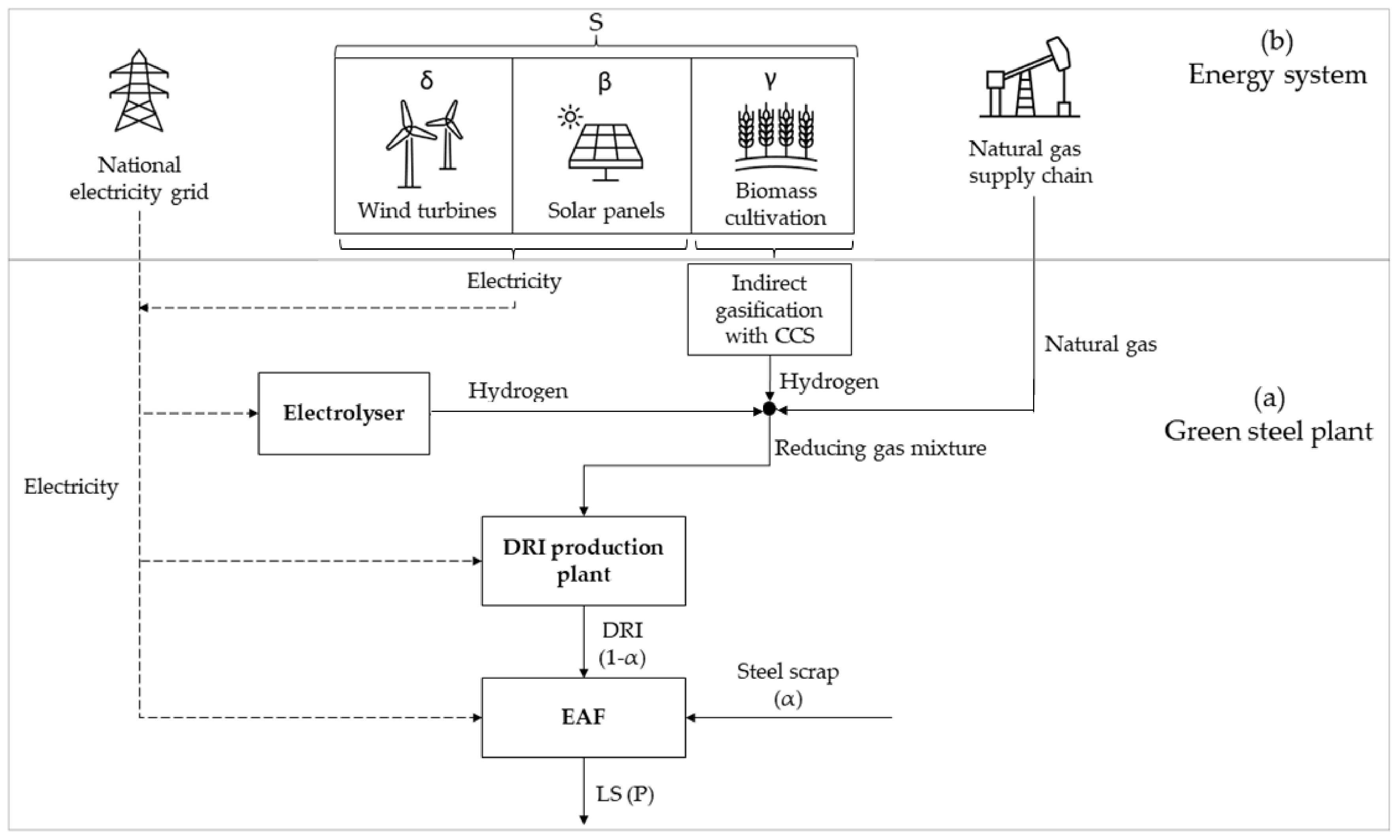
2.1. The Energy System and the Green Steel Plant

The overall green energy–steel system (GESS) under investigation consists of a green steel plant (Figure 1a) and an energy system (Figure 1b) operated in an assigned site.

2.1.1. The Green Steel Plant

The green steel plant (Figure 1a) consists of two main facilities: a DRI plant and an EAF to produce a yearly amount of liquid steel $P [\mathrm{tLS}/\mathrm{y}]$. Gas and electricity utilities feed both technological plants. A reducing gas mixture consisting of natural gas and hydrogen is required to produce DRI. Hydrogen is produced by an electrolyzer having an electricity consumption $E{L}_{H2} [\mathrm{kWh}/{\mathrm{Nm}}^3{\mathrm{H}}_2]$ and/or by a gasification unit. DRI is produced in variable share ($\alpha$) of recycled steel scrap of the overall raw material flow, DRI—steel scraps, feeding the EAF. The DRI plant is fed with the natural gas–hydrogen reducing gas mixture having a volume fraction of hydrogen, $r$. Hydrogen fraction depends on the environmental performance of the energy system, technology adopted for hydrogen production, and steel scraps fraction ($\alpha$). Electricity demand of the whole green steel plant is met primarily by energy produced by renewable energy conversion systems and integrated by the supply from the national electricity grid. Steel-making processes not adopting DRI as virgin material are not considered in the modeled green steel plant, as well as the type of steel to be produced.

2.1.2. The Energy System

The energy system (Figure 1b) consists of national electricity grid and a local renewable energy conversion system. The former system supplies electric energy with almost unlimited capacity; it is characterized by a greenhouse gas emission factor, $f_{grid} [{\mathrm{kgcO}}_{2\mathrm{eq}}/\mathrm{kWh}]$, which depends on the mix of renewable/fossil energy sources of power plants feeding the national grid. The local renewable energy conversion system consists of a wind power plant and/or a photovoltaic plant; both power plants are limited in power capacity as they are installed in an area of limited extension $S \left[{\mathrm{m}}^2\right]$. Wind and solar installations occupy a share of $S$, respectively, $\delta$ and $\beta$. In the same area, cultivated biomass, installed in a share $\gamma$ of $S$, is a feedstock for an indirect gasification process with CCS to produce hydrogen. Wind and photovoltaic power stations are characterized by an average yearly electricity production capacity per unit area and a lifecycle greenhouse gas emission factor per unit of electricity produced $E{S}_w \left[\mathrm{kWh}/{\mathrm{m}}^2·\mathrm{y}], f_w \right[{\mathrm{kgcO}}_{2\mathrm{eq}}/\mathrm{kWh}]$ and $E{S}_{pv} \left[\mathrm{kWh}/{\mathrm{m}}^2·\mathrm{y}], f_{pv} \right[{\mathrm{kgcO}}_{2\mathrm{eq}}/\mathrm{kWh}]$, respectively. As far as the indirect gasification process is concerned, the hydrogen production yield is referred here to the unit area of biomass cultivation, ${\eta }_{bio} [{\mathrm{Nm}}^3{\mathrm{H}}_2/{\mathrm{m}}^2·\mathrm{y}]$, and a lifecycle emission factor per unit of hydrogen produced, $f_{bio} [{\mathrm{kgcO}}_{2\mathrm{eq}}/{\mathrm{Nm}}^3{\mathrm{H}}_2]$, is considered. An electrolysis unit (Figure 1a) powered by the electricity grid integrates hydrogen required by the DRI production process. The energy system also includes a natural gas grid with almost unlimited capacity; natural gas integrates reducing gas required by the DRI production process. The natural gas supply chain is characterized by an emission factor, $f_{CH4} [{\mathrm{kgCO}}_{2\mathrm{eq}}/{\mathrm{Nm}}^3{\mathrm{CH}}_4]$, which considers carbon emissions from gas extraction to transport and utilization. Electricity generated by renewable energy plants or made available by the grid, as well as hydrogen produced by biomass or electrolyzer, are utilities feeding the green steel plant.

2.2. The Analytical Model for the GESS Minimum Emissions Configuration

The model proposed aims at identifying the minimum emission configuration of the energy system and of the green steel plant. Configuration is defined by values assumed by the variables considered in the analytical model (Table 1). Variables can be classified according to two categories (Figure 2):

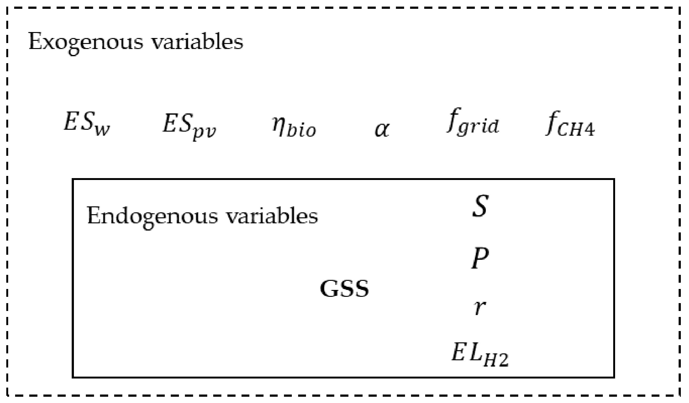
• Exogenous variables: they are variables that cannot be influenced by the decision-maker because of the characteristics of the site where the GESS is expected to be located and the dynamic of the raw materials market. In the context of the present work, the energy and hydrogen producibility per unit area, the share of scrap employed to produce LS in EAF, the national grid emission factor, and the natural gas supply chain emission factor are considered in this category. The amount of energy and hydrogen that can be produced per unit area by renewable energy conversion systems (i.e., wind turbines, solar panels, and gasification plants) depends on the characteristics of the installation site, such as windiness and global solar radiation, and the availability of steel scrap on the market cannot be influenced by the needs of a single plant and, finally, emissions from the electricity grid depend on the national energy mix.
• Endogenous variables: they are variables set by the decision-maker during the plant design phase. In the context of the present work, the total area of the energy system, the volumetric share of hydrogen in the reducing gas of the DRI production process, the electrolyzer technology to be adopted, and the expected yearly production volume of liquid steel are considered in this category since they are characteristic choices of a plant design.

In accordance with the GHG protocol [34], the overall emissions of the system consist of

$${\phi }_{tot} \left[\frac{{\mathrm{kgCO}}_{2\mathrm{eq}}}{\mathrm{tLS}}\right]={\phi }_{direct}+{\phi }_{indirect}$$

(1)

where

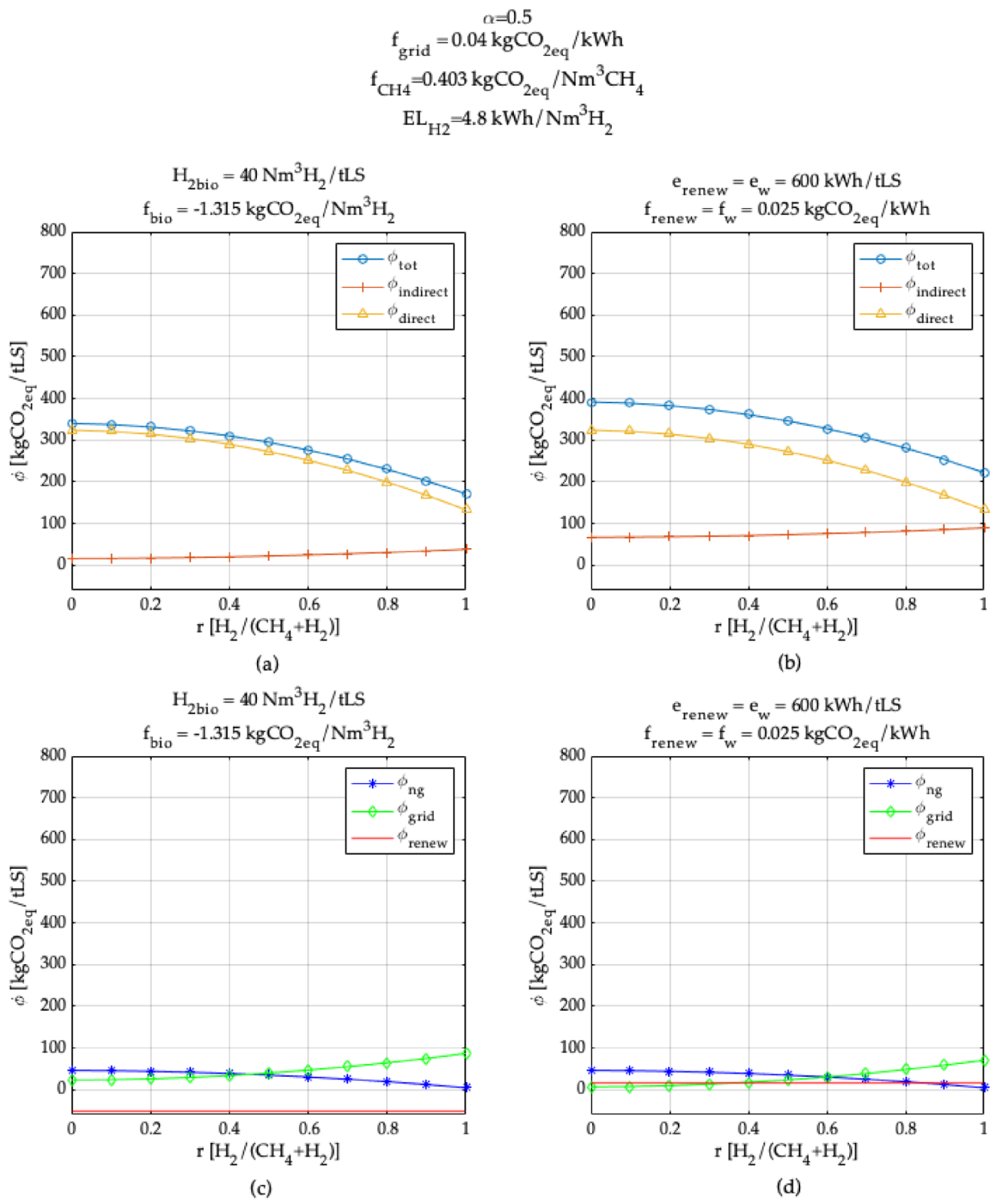
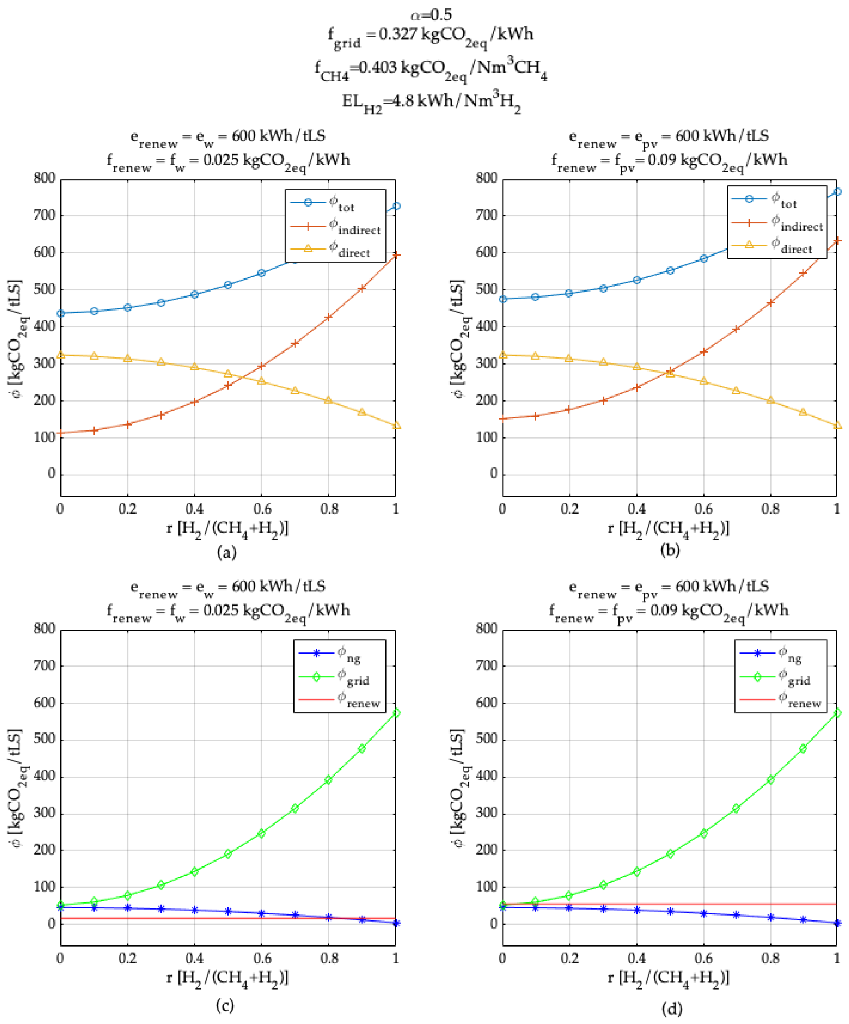
• ${\phi }_{direct} \left[\frac{{\mathrm{kgCO}}_{2\mathrm{eq}}}{\mathrm{tLS}}\right]$: direct emissions generated by the green steel plant. “direct GHG emissions” are defined as GHG emissions generated in owned or controlled process equipment [34]. In the green steel plant, direct emissions are from DRI plant with an emission factor, $f_{DRI}\left(r\right)$, and from the EAF. Different EAF emission factors in case of scraps or DRI feeding it are considered ($f_{EAFSCRAP}$ and $f_{EAFDRI}$, respectively).
• ${\phi }_{indirect} \left[\frac{{\mathrm{kgCO}}_{2\mathrm{eq}}}{\mathrm{tLS}}\right]$: emissions generated by the production of electricity and the supply of natural gas to power the DRI process. As established by the GHG protocol [34], “electricity indirect emissions and other GHG emissions” are defined as emissions deriving from the production of electricity consumed by the plant and from activities that can be considered a consequence of the plant’s activity, e.g., the extraction and transport of raw materials. The characteristic of indirect emissions is that, although they do not physically occur at the plant site, they have a significant influence on the total account of the emissions generated. In the case of the analyzed system, lifecycle emissions related to renewable energy conversion systems to produce electricity and hydrogen, emissions related to the production of electricity fed into the national grid ($f_{grid}$), and emissions generated by the natural gas supply chain to power the DRI production process ($f_{CH4}$) have been considered in this category. As far as emissions related to renewable energy and biomass conversion systems are considered, lifecycle emissions have been taken into reference as, on the one hand, all stages of the lifecycle of wind turbines and photovoltaic panels, from production to decommissioning, have been considered ($f_w, f_{pv}$), while, on the other hand, consideration of the carbon sink associated with the growth of biomass has been included ($f_{bio}$). In this paper, emissions due to iron ore extraction and scrap transport have not been included in the model as they represent invariant variables in the optimization process.

Direct emissions of Equation (1) can be evaluated as

$${\phi }_{direct}\left[\frac{{\mathrm{kgCO}}_{2\mathrm{eq}}}{\mathrm{tLS}}\right]=\left(1-\alpha \right)·\left(\frac{f_{DRI}\left(r\right)}{k}+f_{EA{F}_{DRI}}\right)+\alpha ·f_{EA{F}_{SCRAP}}$$

(2)

Direct emissions include emissions from the DRI production process and EAF emissions, weighted on the share ($\alpha$) of recycled steel scrap employed to produce liquid steel. Direct emissions from the EAF have a different value, depending on whether recycled steel scrap ($f_{EA{F}_{SCRAP}}$) or DRI ($f_{EA{F}_{DRI}}$) feeds the furnace [24]. The direct emissions generated by the DRI production process have been considered as a function of the volumetric share of hydrogen in the reducing gas ($f_{DRI}\left(r\right)$).

Indirect emissions can be calculated as

$${\phi }_{indirect} \left[\frac{{\mathrm{kgCO}}_{2\mathrm{eq}}}{\mathrm{tLS}}\right]={\phi }_{NG}+{\phi }_{renewables}+{\phi }_{grid}$$

(3)

where

$${\phi }_{NG} \left[\frac{{\mathrm{kgCO}}_{2\mathrm{eq}}}{\mathrm{tLS}}\right]=\left(1-\alpha \right)·\frac{C{H}_4\left(r\right)}{k}·f_{CH4}$$

(4)

Equation (4) allows evaluating the indirect emissions generated by the supply of natural gas for the DRI production process. These emissions have been accounted only for the DRI share employed to produce LS ($1-\alpha$); moreover, the natural gas requirement has been considered as function of the volumetric share of hydrogen in the reducing gas ($C{H}_4\left(r\right)$).

$${\phi }_{renewables }\left[\frac{{\mathrm{kgCO}}_{2\mathrm{eq}}}{\mathrm{tLS}}\right]=\frac{S·\left(\delta ·E{S}_w·f_w+\beta ·E{S}_{pv}·f_{pv}+\gamma ·{\eta }_{bio}·f_{bio}\right)}{P}$$

(5)

In Equation (5), the indirect emissions generated by the energy system producing electricity and hydrogen are computed. As can be observed, global emissions mainly depend on the total area committed to the energy system ($S$) as well as on the shares of the area dedicated to the installation of the considered renewable energy conversion systems ($\delta ,\beta$) and the cultivation of biomass ($\gamma$). These indirect emissions also depend on the producibility of energy and hydrogen per unit area for each of the alternatives considered ($E{s}_w,E{s}_{pv},{\eta }_{bio}$).

$${\phi }_{grid}\left[\frac{{\mathrm{kgCO}}_{2\mathrm{eq}}}{\mathrm{tLS}}\right]=[E_{demand}-\frac{S·\left(\delta ·E{S}_w+\beta ·E{S}_{pv}\right)}{P}]·f_{grid}$$

(6)

Equation (6) models the indirect emissions related to the supply of electricity from the national grid, with a characteristic emission factor $f_{grid}$. In (6), the electricity supplied from the national grid is evaluated as the amount required by the steel system and not satisfied by the energy system. The more electricity produced by the energy system, therefore, the lower the emissions generated by the supply of electricity from the national grid.

Energy demand of the green steel plant (in Equation (6)) is given by

$$E_{demand} \left[\frac{\mathrm{kWh}}{\mathrm{tLS}}\right]=\left[\left(1-\alpha \right)·\left(E{L}_{AUX}+E{L}_{EA{F}_{DRI}}\right)+\alpha ·E{L}_{EA{F}_{SCRAP}}+\left(\left(1-\alpha \right)·\frac{H_2\left(r\right)}{k}-\frac{\gamma ·S·{\eta }_{bio}}{P}\right)·E{L}_{H2}\right]$$

(7)

The energy demand from the plant has been also weighted according to the share of recycled steel scrap used for the production of liquid steel ($\alpha$), and two different electricity consumptions of the EAF have been considered ($E{L}_{EA{F}_{DRI}},E{L}_{EA{F}_{SCRAP}}$), depending on whether DRI or scrap is processed. The hydrogen requirement to supply the DRI production process has been considered as a function of the volumetric share of hydrogen used in the reducing gas ($H_2\left(r\right)$). The electrical requirement to produce hydrogen from electrolyzer has been considered for the share of the total hydrogen requirement not produced by indirect gasification of biomass.

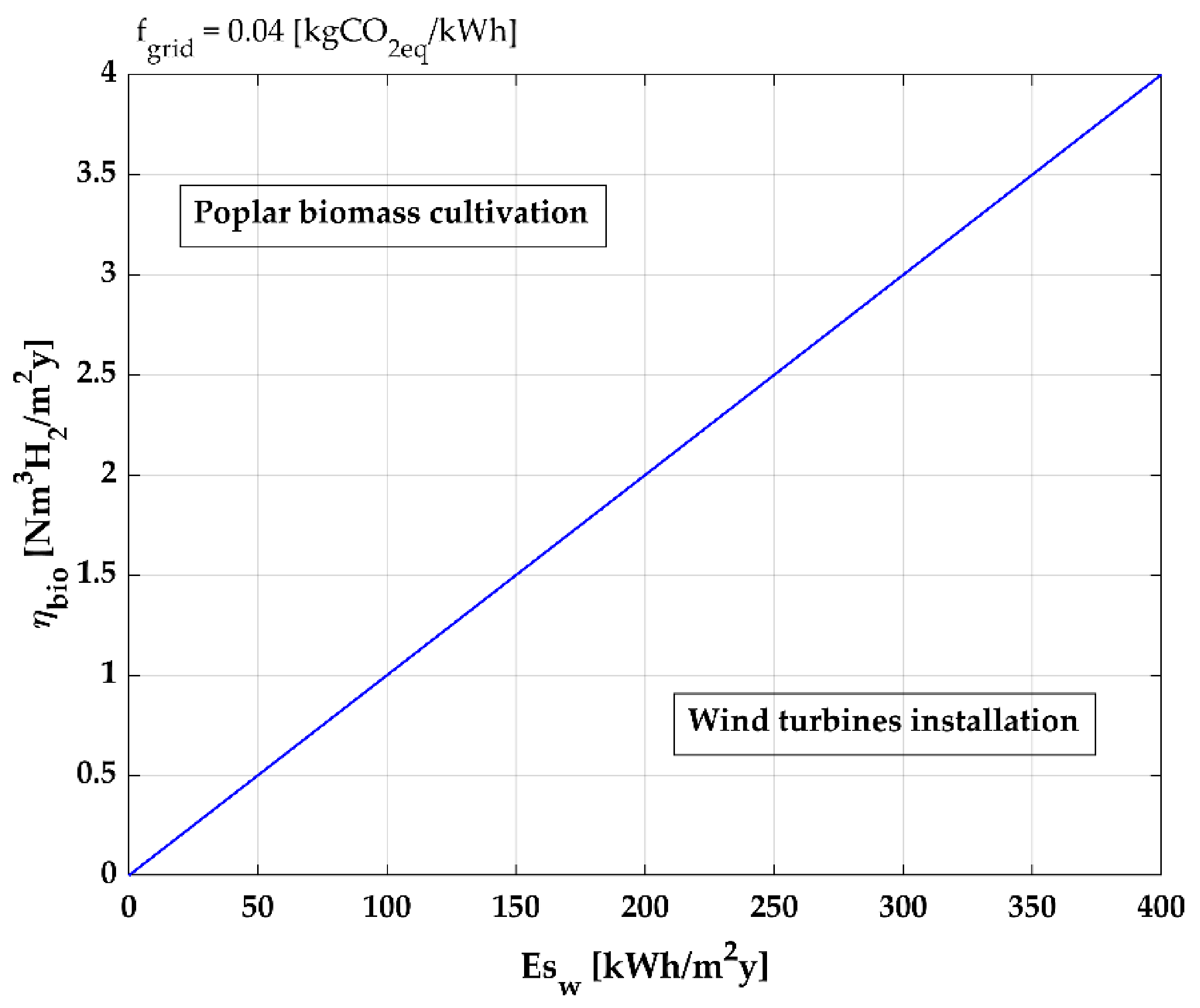
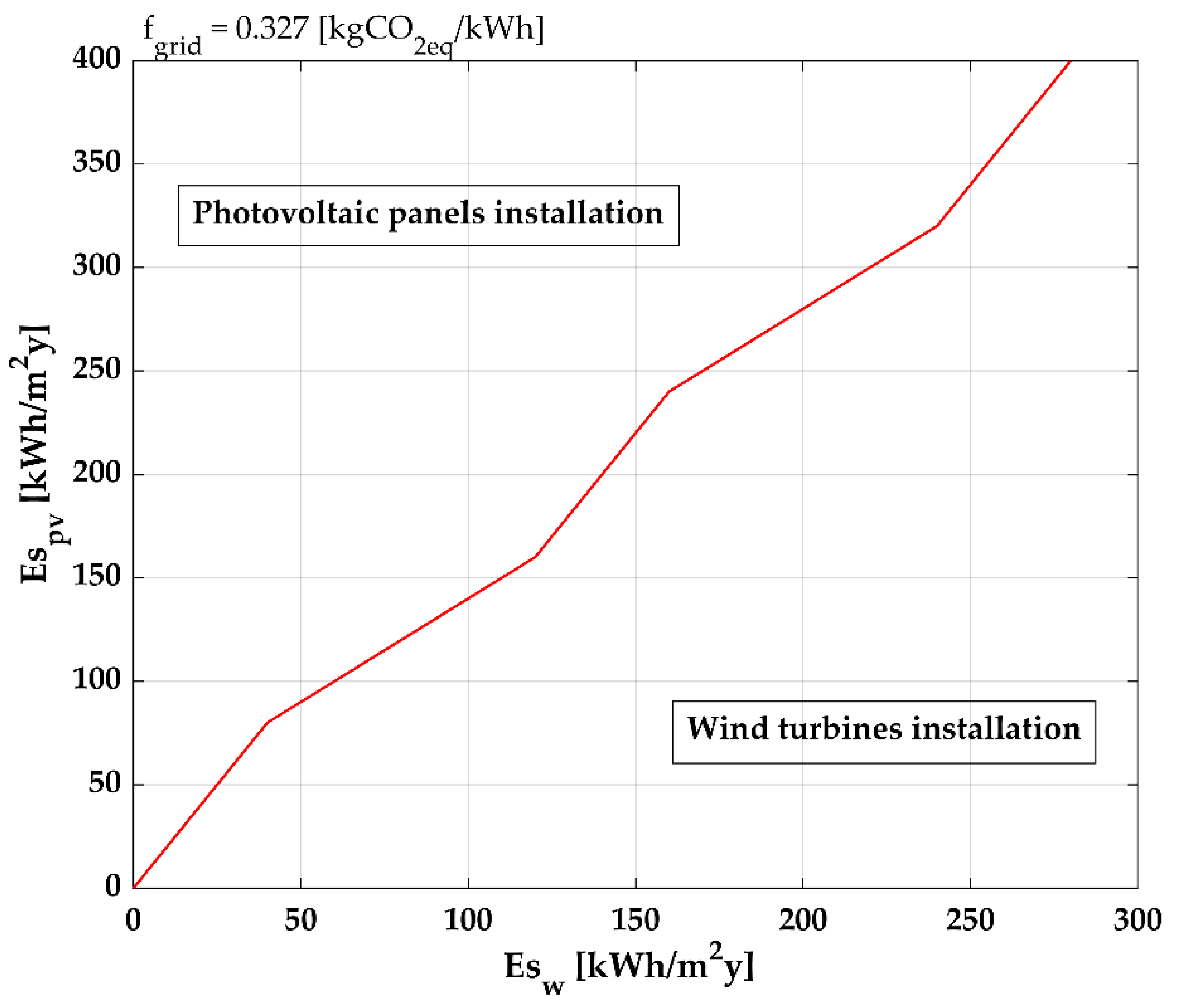
2.3. Avoided Grid Emissions by the Renewable Energy System

As shown in Equation (3), indirect emissions of the system consist of three contributions: emissions due to natural gas supply chain as well as to grid and renewable sources operation to produce electricity or hydrogen. The more electricity that is produced by the renewable energy system, the lower the grid emissions are (Equation (6)). For this reason, it is possible to compare the environmental effectiveness of renewable energy conversion and hydrogen production systems on the basis of the avoided emissions. For this purpose, avoided emissions for each of the i-th renewable energy systems (i = wind, solar, biomass) are computed per unit installation area ($A{v}_{e{m}_i}$) as the product of the i-th electricity yield ($E{s}_i$) and of the difference between the grid emission factor ($f_{grid}$) and the lifecycle emissions factor of the i-th alternative ($f_i$) (Equation (8)).

$$A{v}_{e{m}_i}\left[\frac{{\mathrm{kgCO}}_2}{{\mathrm{m}}^2·\mathrm{y}}\right]=E{S}_i·f_{grid}-E{S}_i·f_i=E{S}_i·\left(f_{grid}-f_i\right)$$

(8)

In the case of hydrogen production, the avoided emissions are calculated with reference to the production of hydrogen from the electrolyzer powered by the grid. Avoided emissions per unit area in case of the alternatives considered are in Equations (9)–(11):

$$A{v}_{e{m}_w}\left[\frac{{\mathrm{kgCO}}_2}{{\mathrm{m}}^2·\mathrm{y}}\right]=E{S}_w·\left(f_{grid}-f_w\right)$$

(9)

$$A{v}_{e{m}_{pv}}\left[\frac{{\mathrm{kgCO}}_2}{{\mathrm{m}}^2·\mathrm{y}}\right]=E{S}_{pv}·\left(f_{grid}-f_{pv}\right)$$

(10)

$$A{v}_{e{m}_{bio}}\left[\frac{{\mathrm{kgCO}}_2}{{\mathrm{m}}^2·\mathrm{y}}\right]={\eta }_{bio}·\left(E{L}_{H2}·f_{grid}-f_{bio}\right)$$

(11)

Since $f_{grid}$, $E{s}_w$, $E{s}_{pv}$, and ${\eta }_{bio}$ are exogenous variables, they are not subjected to optimization; their values depend on the GESS site location characteristics (e.g., average windiness, solar global radiation, cultivation yield) as well as on technology factors such as the electricity consumption of the electrolyzer and the national grid emission factor.

For a given renewable energy system, avoided emissions differ at each location. For a given location, avoided emissions vary on the basis of the renewable energy system adopted:

$$E{S}_w·\left(f_{grid}-f_w\right)\ne E{S}_{pv}·\left(f_{grid}-f_{pv}\right)\ne {\eta }_{bio}·\left(E{L}_{H2}·f_{grid}-f_{bio}\right)$$

(12)

As an example, in case of

$$E{S}_w·\left(f_{grid}-f_w\right)>E{S}_{pv}·\left(f_{grid}-f_{pv}\right)>{\eta }_{bio}·\left(E{L}_{H2}·f_{grid}-f_{bio}\right)$$

(13)

being

$$\delta +\beta +\gamma =1 \mathrm{with} 0\le \delta ,\beta ,\gamma \le 1$$

(14)

then,

$$\begin{gathered} S·E{S}_w·\left(f_{grid}-f_w\right)\ge S·\delta ·E{S}_w·\left(f_{grid}-f_w\right)+S·\beta ·E{S}_{pv}·\left(f_{grid}-f_{pv}\right)+ \\ +S·\gamma ·{\eta }_{bio}·\left(E{L}_{H2}·f_{grid}-f_{bio}\right) \end{gathered}$$

(15)

In this case, maximum avoided emissions are obtained with $\delta =1, \beta =0, \gamma =0$. Therefore, only one out of the three renewable energy system alternatives has to be considered as the best alternative from an environmental point of view for a specific site. In accordance, Equations (5)–(7) can be rearranged as

$${\phi }_{renew}\left[\frac{{\mathrm{kgCO}}_{2\mathrm{eq}}}{\mathrm{tLS}}\right]=e_{renew}·f_{renew}+H_{2bio}·f_{bio}$$

(16)

$${\phi }_{grid}\left[\frac{{\mathrm{kgCO}}_{2\mathrm{eq}}}{\mathrm{tLS}}\right]=[E_{demand}-e_{renew}]·f_{grid}$$

(17)

$$E_{demand} \left[\frac{\mathrm{kWh}}{\mathrm{tLS}}\right]=\left[\left(\left(1-\alpha \right)·\left(E{L}_{AUX}+E{L}_{EA{F}_{DRI}}\right)+\alpha ·E{L}_{EA{F}_{SCRAP}}\right)+\left(\left(1-\alpha \right)·\frac{H_2\left(r\right)}{k}-H{2}_{bio}\right)·E{L}_{H2}\right]$$

(18)

where

$$e_{renew}=\delta ·\frac{S·E{S}_w}{P}+\beta ·\frac{S·E{S}_{pv}}{P}$$

(19)

$$f_{renew}=\delta ·f_w+\beta ·f_{pv}$$

(20)

$$H_{2bio}=\gamma ·\frac{S·{\eta }_{bio}}{P}$$

(21)

with $\delta ,\beta ,\gamma ϵ\left\{0;1\right\} \wedge \delta +\beta +\gamma =1$.

In the next section it is shown how to apply the model in order to identify the minimum emissions configuration of a green energy–steel system for a given site location. Moreover, results of numerical simulations and sensitivity analysis are presented.

3. Model Application

Figure 3 shows the procedure for applying the model in order to identify the minimum emission configuration of the GESS considered.

Once the site location for the GESS’s installation has been identified, the values of the variables $E{S}_w, E{S}_{pv}, {\eta }_{bio}, f_{grid}$ can be obtained. It is also necessary to choose the electrolyzer technology to be adopted ($E{L}_{H2}$). From these data it is possible to evaluate the avoided emissions from the electricity grid for each of the renewable energy system alternatives considered (Equations (9)–(11)), and to identify the one that provides the highest contribution. Depending on the specific context, therefore, it is possible to identify which one among the variables $\delta , \beta , \gamma$should assume value 1, i.e., which one among the renewable energy conversion systems is considered to be installed. By choosing the liquid steel annual production capacity $P$, and the area $S$ to be dedicated to the installation of the renewable energy conversion system identified, it is possible to calculate the values of $e_{renew}$ (Equation (19)), $f_{renew}$ (Equation (20)), $H_{2bio}$ (Equation (21)), and finally ${\phi }_{renew}$ (Equation (16)). The share of available steel scrap with respect to annual requirements ($\alpha$) can be obtained by market analysis. By assuming the values of the variables $k, f_{CH4}, E{L}_{EA{F}_{SCRAP}}, E{L}_{EA{F}_{DRI}}, E{L}_{AUX}, f_{EAF{S}_{SCRAP}}, f_{EA{F}_{DRI}}$, it is possible to calculate the value of the total emission function ${\phi }_{tot}$ (Equation (16)) and to find the optimal value of the volumetric share of hydrogen in the reducing gas mixture to be adopted in the DRI production process ($r$), minimizing emissions.

Figure 4 and Figure 5 illustrate the results obtained from the numerical simulations carried out by calculating the avoided emissions in two scenarios corresponding to two different values of $f_{grid}$ (corresponding to the 2019 Italian and French energy mix). In both cases, avoided emissions have been calculated for each of the energy system alternatives considered (Equations (9)–(11)) by varying specific electricity/hydrogen producibility values ($E{S}_w, E{S}_{pv}$, ${\eta }_{bio}$) with the aim of identifying the renewable energy conversion systems to be installed (Figure 3) to maximize avoided emissions.

Results obtained in the case of $f_{grid}=0.04{ \mathrm{kgCO}}_{2\mathrm{eq}}/\mathrm{kWh}$ are shown in Figure 4. As can be observed, in this scenario, there are only two alternatives to choose from for the energy system configuration, i.e., wind turbines and poplar biomass cultivation ($\delta =1$ or $\gamma =1$). In this scenario, installation of photovoltaic panels is never representative of the best alternative since photovoltaic emission factor ($f_{pv}$) is higher than the grid one ($f_{grid}$). For each site it possible to identify a point $p$ $\left(E{S}_w,{\eta }_{bio}\right)$ located in a region of the plane characterized by an optimal solution, corresponding to the energy system configuration to be adopted. If the point $p$ belongs to the line in the graph, the two energy conversion systems (wind, biomass) lead to the same environmental benefit.

Figure 5 shows the results obtained in case of $f_{grid}=0.327{ \mathrm{kgCO}}_{2\mathrm{eq}}/\mathrm{kWh}$. Differently to the previous case, the two alternatives to choose from in this scenario are wind turbines and photovoltaic panels ($\delta =1$ or $\beta =1$). Although biomass cultivation always offers positive avoided emissions (it has a negative characteristic emission factor $f_{bio}$; Equation (11)), it never results as the best alternative since significant avoided emissions are from the production of electricity from energy conversion systems. Additionally, in this case, depending on the $E{S}_w,E{S}_{pv}$ values of the site under analysis, it is possible to identify a point $p$ of $\left(E{s}_w,E{s}_{pv}\right)$ coordinates, located in a region of the plane characterized by an optimal solution, corresponding to the energy system configuration to be adopted.

According to the results obtained, it is noteworthy that the only scenario in which biomass cultivation could be the best alternative is the one characterized by $f_{grid}=0.04{ \mathrm{kgCO}}_{2\mathrm{eq}}/\mathrm{kWh}$. This implies that the starting condition represented by a particularly “green” national energy mix is required to trigger a mechanism of synergic relations between green steel production and the supporting public infrastructure. Once the best solution has been identified (Equations (9)–(11)), and the values of $S$ and $P$ have been chosen, the values of $e_{renew}$ (Equation (19)), $f_{renew}$ (Equation (20)), $H_{2bio}$ (Equation (21)), and ${\phi }_{renew}$ (Equation (16)) are calculated (Figure 3). According to the results obtained (Figure 4 and Figure 5), it is noteworthy that only in the scenario characterized by $f_{grid}=0.04{ \mathrm{kgCO}}_{2\mathrm{eq}}/\mathrm{kWh}$, can the value of ${\phi }_{renew}$ be negative, with biomass cultivation being a possible best alternative.

Once the energy system has been optimally configured, it is possible to size the green steel plant (Figure 3). First, based on available market data, the maximum availability of recycled steel scrap must be identified ($\alpha$). The more recycled steel scrap that can be used to feed the EAF (i.e., as close as possible to a theoretical secondary route), the more the sustainable steel production is considered from an environmental point of view. In this way, a valuable resource (scrap) can be placed back into the production cycle, avoiding the consumption of energy and raw materials associated with the production of DRI. Figure 6 shows the trend of total emissions ${\phi }_{tot}$ as a function of the $\alpha$ variable in different scenarios. The value of the remaining variables (i.e., $k, f_{CH4}, E{L}_{EAFSCRAP}, E{L}_{EAFDRI}, E{L}_{AUX}, f_{EAFSCRAP}, f_{EAFDRI}$) has been set according to Table 1.

The scenarios have been built up according to the results obtained from the preview simulations. Electricity production from wind turbines (Figure 6b) and biomass cultivation (Figure 6a) have been considered in the case of $f_{grid}=0.04{ \mathrm{kgCO}}_{2\mathrm{eq}}/\mathrm{kWh}$, and electricity production from wind turbines (Figure 6c) or photovoltaic panels (Figure 6d) in the case of $f_{grid}=0.327{ \mathrm{kgCO}}_{2\mathrm{eq}}/\mathrm{kWh}$. The trend of ${\phi }_{tot}$ has been evaluated in the case of a reducing gas consisting of only hydrogen ($r=1$) or natural gas ($r=0$). As can be observed, in all cases, ${\phi }_{tot}$ decreases as the value of $\alpha$ increases. For this reason, it is advisable to maximize the value of this variable as much as possible (consistently with market availability) when sizing the green steel plant. It can also be observed that, in the case of national “green” electricity production ($f_{grid}=0.04{ \mathrm{kgCO}}_{2\mathrm{eq}}/\mathrm{kWh}$), the value of total emissions is significantly lower than in the case of $f_{grid}=0.327{ \mathrm{kgCO}}_{2\mathrm{eq}}/\mathrm{kWh}$. Finally, it is noteworthy that, in the scenarios characterized by $f_{grid}=0.327{ \mathrm{kgCO}}_{2\mathrm{eq}}/\mathrm{kWh}$, there is a significant gap between the emissions in the cases of $r=1$ and $r=0$. At $\alpha =0$ and $f_{grid}=0.327{ \mathrm{kgCO}}_{2\mathrm{eq}}/\mathrm{kWh}$, indeed, emissions at $r=1$ are about 125% higher than at $r=0$, while at $\alpha =0$ and $f_{grid}=0.04{ \mathrm{kgCO}}_{2\mathrm{eq}}/\mathrm{kWh}$, the difference is about 8%. This highlights the relevance of emissions generated by the supply of energy for hydrogen production with respect to the GESS’s total emissions. It is, therefore, possible to observe how, in the presence of favorable infrastructural conditions (i.e., low value of $f_{grid}$), synergies are generated and the production of steel using hydrogen is favored.

After assigning (endogenous) or deriving (exogenous) values for all variables through the illustrated procedure (Figure 3), the objective is to identify the value of $r$ that minimizes the total emissions function ${\phi }_{tot}$. It is not possible to predict whether the value of this variable should be minimized or maximized (as in the case of $\alpha$, which should be maximized in all cases), since increasing $r$ generates the opposite effects in the contributions that constitute the total emissions function (Figure 7).

As can be observed from Figure 7, the direct emissions from the DRI production plant ($f_{DRI}\left(r\right)$) and the demand of natural gas for the reducing gas ($C{H}_4\left(r\right))$ decrease as $r$ increases, while the demand for hydrogen ($H_2\left(r\right)$) increases. It is also possible to observe that the demand for hydrogen and methane reach the same value near to r = 0.5 and then the demand for hydrogen increases more than the demand for methane decreases. This is because hydrogen has a lower reducing power compared to methane. To this concern, Figure 8 and Figure 9 show the trend of ${\phi }_{tot}$ and its components (i.e., ${\phi }_{direct}, {\phi }_{NG}, {\phi }_{grid}, {\phi }_{renew}$ according to Equations (2), (3), (16), and (17)) as functions of the $r$ variable.

Additionally in this case, different scenarios have been built up according to the results obtained from the preview simulations. Figure 8 shows the results obtained in the case of $f_{grid}=0.04{ \mathrm{kgCO}}_{2\mathrm{eq}}/\mathrm{kWh}$, and Figure 9 shows the results obtained in the case of $f_{grid}=0.327{ \mathrm{kgCO}}_{2\mathrm{eq}}/\mathrm{kWh}$. Electricity production from wind turbines (Figure 8b,d) and biomass cultivation (Figure 8a,c) have been considered in the case of $f_{grid}=0.04{ \mathrm{kgCO}}_{2\mathrm{eq}}/\mathrm{kWh}$, and electricity production from wind turbines (Figure 9a,c) or photovoltaic panels (Figure 9b,d) in the case of $f_{grid}=0.327{ \mathrm{kgCO}}_{2\mathrm{eq}}/\mathrm{kWh}$. As can be observed, the ${\phi }_{tot}$ function decreases in scenarios with $f_{grid}=0.04{ \mathrm{kgCO}}_{2\mathrm{eq}}/\mathrm{kWh}$ (Figure 8), while it increases in scenarios with $f_{grid}=0.327{ \mathrm{kgCO}}_{2\mathrm{eq}}/\mathrm{kWh}$ (Figure 9). The values of emissions observed in the first case (Figure 8a,b) are significantly lower than those observed in the second case (Figure 9a,b). As far as the contributions that constitute ${\phi }_{tot}$ (Equation (1)) are concerned, it is possible to observe that in all the scenarios considered (Figure 8 and Figure 9), ${\phi }_{direct}$ and ${\phi }_{NG}$ decrease as $r$ increases, while ${\phi }_{grid}$ increases. The most significant difference is observed in the latter contribution. In Figure 8c,d, the maximum value of ${\phi }_{grid}$(at $r=1$) is slightly below 100 ${\mathrm{kgCO}}_{2\mathrm{eq}}/\mathrm{tLS}$, while in Figure 9c,d, it is higher than 600 ${\mathrm{kgCO}}_{2\mathrm{eq}}/\mathrm{tLS}$. This confirms that the emissions generated by electricity consumption for hydrogen production are significant and that, consequently, sustainable energy production from the grid allows for green steel production.

Regarding the numerical simulations carried out to find the optimal value of $r$ minimizing the overall emissions from the GESS by varying $f_{grid}$, it has been found that, for any combination of values of the considered variables (Figure 2), overall emission function (${\phi }_{tot}$) does not admit a minimum for any $r$ value.

For specific values of $f_{grid}$, indeed, the function has a monotonic trend; if it is monotonically increasing, minimum emissions are obtained in the case of $r=0$ (e.g., $f_{grid}=0.22 {\mathrm{kgCO}}_{2\mathrm{eq}}/\mathrm{kWh}$); if it is monotonically decreasing, minimum emissions are obtained in the case of $r=1$ (e.g., $f_{grid}=0.1 {\mathrm{kgCO}}_{2\mathrm{eq}}/\mathrm{kWh}$). When the function is not monotonic (e.g., $f_{grid}=0.13 {\mathrm{kgCO}}_{2\mathrm{eq}}/\mathrm{kWh}$), it does not show a minimum, which confirms that for all $f_{grid}$ values, minimum emissions are obtained in the cases of $r=0$ or $r=1$, and not in intermediate values ($0<r<1$). From the results obtained (Figure 10), it can be observed that the feasibility of installing a hydrogen-powered steel plant ($r=1$) is determined, from an environmental point of view, only by the $f_{grid}$ value, i.e., by the way in which electricity is produced at national level. Additionally in this case, it can be observed that low $f_{grid}$ values generate synergies in the GESS that allow the decrease of ${\phi }_{tot}$ as the share of hydrogen produced increases ($r$). The other variables considered (e.g., $\alpha , e_{renew}, P, S$, etc.) affect emissions in terms of absolute value, but do not influence the choice of DRI production mode ($r=0$ or $r=1$). At $r=0$, there is no significant difference between the ${\phi }_{tot}$ values recorded at the minimum and the maximum $f_{grid}$ values considered. The situation is completely different at $r=1$, at which there is a very significant difference between the values of ${\phi }_{tot}$at minimum $f_{grid}$ and maximum $f_{grid}$ considered. For example, in the case of electricity production from wind turbines (Figure 10b), at $r=0$, there is an increase of 13.18% from the ${\phi }_{tot}$ value at $f_{grid}=0.01 {\mathrm{kgCO}}_{2\mathrm{eq}}/\mathrm{kWh}$, compared with $f_{grid}=0.327 {\mathrm{kgCO}}_{2\mathrm{eq}}/\mathrm{kWh}$, while at $r=1$, the increase is 324.6%. This confirms that electricity consumption for hydrogen production constitutes the most significant share of total emissions and that, therefore, it is necessary to assess the feasibility of GESS installation according to the reference context. However, the results showed that steel production with alternative route (DRI–EAF), regardless of the component of the DRI reducing gas ($r$), is environmentally favourable. At $r=0$, indeed, there is a significant reduction in emissions compared to the BF–BOF route in each scenario, which can even become more significant in contexts where it is convenient to produce with only hydrogen (Figure 10). Referring to Figure 10b, it can be observed that ${\phi }_{tot}$ values at $r=0$ are around 400 ${\mathrm{kgCO}}_{2\mathrm{eq}}/\mathrm{tLS}$, 83.34% less than the BF–BOF route, whereas at $r=1$, the minimum value recorded is 171 ${\mathrm{kgCO}}_{2\mathrm{eq}}/\mathrm{tLS}$, 90.5% less than the conventional alternative. It is noteworthy that even at the worst scenario, i.e., $f_{grid}=0.327 {\mathrm{kgCO}}_{2\mathrm{eq}}/\mathrm{kWh}$ and $r=1$, the emissions are 726 ${\mathrm{kgCO}}_{2\mathrm{eq}}/\mathrm{tLS}$, 59.6% less than the primary route, thus proving the effectiveness of the DRI–EAF route.

From the observation made on the trend of ${\phi }_{tot}$ with respect to $r$ (Figure 10), it has been therefore possible to calculate the value of $f_{grid}$ that makes equal the value of ${\phi }_{tot}$ at $r=0$ and $r=1$, called $f_{grid}”$ (Equation 22). This is the maximum value of the grid emission factor at which it is environmentally convenient to install a hydrogen-powered steel plant ($r=1$). The analytical expression of $f_{grid}”$ is

$$f_{grid}”\left(r\right)\left[\frac{{\mathrm{kgCO}}_{2\mathrm{eq}}}{\mathrm{kWh}}\right]=\frac{\left({\phi }_{direct}\left(1\right)+{\phi }_{NG}\left(1\right)\right)-\left({\phi }_{direct}\left(0\right)+{\phi }_{NG}\left(0\right)\right)}{\left(E_{demand}\left(0\right)-e_{renew}\right)-\left(E_{demand}\left(0\right)-e_{renew}\right)}$$

(22)

The expression in Equation (22) is a function of the variables $f_{CH4}$ and $E{L}_{H2}$. As the first variable is exogenous, the trend of $f_{grid}”$ has been studied as a function of the only endogenous variable $E{L}_{H2}$ (Figure 11).

As it can be observed in Figure 11, $f_{grid}”$ decreases as the electrical consumption of the electrolyzer increases. In the figure, electricity consumption of the main electrolyzers’ technologies is shown (vertical lines). To this concern, it is therefore possible to observe that for $E{L}_{H2}$ characteristics of the solid oxide electrolyzer (SOEC) technology (4.5 $\mathrm{kWh}/{\mathrm{Nm}}^3{\mathrm{H}}_2$ [23]), currently developed on a lab-scale, the maximum value of $f_{grid}$ at which a hydrogen-powered steelmaking plant can be installed ($f_{grid}”$) is 0.155 ${\mathrm{kgCO}}_{2\mathrm{eq}}/\mathrm{kWh}$. For the alkaline and anion exchange membrane (AEM) technologies, which have very similar average electricity consumption (around 5.7 $\mathrm{kWh}/{\mathrm{Nm}}^3{\mathrm{H}}_2$ [23]), the value of $f_{grid}”$ decreases to approximately 0.122 ${\mathrm{kgCO}}_{2\mathrm{eq}}/\mathrm{kWh}$. Finally, for the polymer electrolyte membrane (PEM) technology (commercially available technology), which has the highest electricity consumption (6 $\mathrm{kWh}/{\mathrm{Nm}}^3{\mathrm{H}}_2$ [23]), the value of $f_{grid}”$ further decreases to about 0.12 ${\mathrm{kgCO}}_{2\mathrm{eq}}/\mathrm{kWh}$. From the overall results obtained, therefore, it is possible to conclude that the installation of a hydrogen-powered steel plant ($r=1$) is only feasible if supported by both technological innovations and supporting infrastructure. The choice of an electrolyzer characterized by low energy consumption and a national energy mix with a low environmental impact represent favorable conditions for the installation of a hydrogen-powered steel plant, thus allowing the decarbonization of the steelmaking sector.

4. Conclusions

The objective of the present work was to develop an analytical model for the identification of the minimum emission configuration of a green energy steel production system (GESS) consisting of a direct reduced iron–electric arc furnace (DRI–EAF) route and a renewable energy system. The model allows to evaluate the feasibility of the installation of a hydrogen-powered steel plant, considering the site location of the system.

Results of simulation carried out show that, regardless of the site location, the installation of GESS is a viable alternative for the decarbonization of the steelmaking process. Depending on the characteristics of the site, decreases in emissions ranging from 60% to 91%, compared to the blast furnace–basic oxygen furnace (BF–BOF) route, can be obtained. The GESS that offers the maximum reduction in global emissions compared to the BF–BOF route (91%) is in a site characterized by green energy mix ($f_{grid}=0.01 {\mathrm{kgCO}}_{2\mathrm{eq}}/\mathrm{kWh}$), whose energy system is dedicated to the cultivation of biomass for hydrogen production through indirect gasification. In this case, the best solution was identified at $r=1$, i.e., a DRI process totally fed by hydrogen. The configuration of the GESS that resulted as the least performing was characterized by less green energy mix ($f_{grid}=0.327{ \mathrm{kgCO}}_{2\mathrm{eq}}/\mathrm{kWh}$) and by the production of hydrogen from the cultivation of biomass in the energy system. In this case, the best solution was identified at $r=0$, i.e., a DRI process totally fed by NG. Although, in this case, the lack of electricity production from renewable sources results in a more significant amount of emissions, there are still significant savings compared to the BF–BOF route. From the analysis carried out, it was also shown that, depending on the reference scenario, the solutions that minimize the overall emissions of the system are those in which only hydrogen or only natural gas (NG) are employed in the DRI reducing gas ($r=0$ or $r=1$), although the emission values recorded in the case of hydrogen are significantly lower than in the case of NG. It indeed resulted that, for any combination of values of the variables considered, the overall emission function modeled does not admit a minimum for any r value. Emission factor from the national electricity proved to be the factor mainly influencing the choice between an all-NG or all-hydrogen system. The lower the value of this factor, indeed, the greener the energy mix employed at a national level and the more favorable the use of hydrogen in the steelmaking process. A low value of emission factor from the national electricity ($f_{grid}-{\mathrm{kgCO}}_{2\mathrm{eq}}/\mathrm{kWh}$) also makes environmentally convenient the production of hydrogen from renewable sources (i.e., biomasses) which has negative overall emissions. Finally, it has been observed that a further variable that significantly influences the environmental feasibility of installing a hydrogen-powered steelmaking route is the electricity consumption of the electrolyzer ($E{L}_{H2}-\mathrm{kWh}/{\mathrm{Nm}}^3{\mathrm{H}}_2$). To this concern, the maximum value of the grid emission factor at which it results as environmentally convenient to install a hydrogen-powered steel plant was studied as a function of the electrical consumption of the electrolyzer. It was observed that, depending on the technology adopted for the electrolyzer, different upper-limit values of the emission factor from the national grid make the hydrogen steelmaking route the best environmental alternative. As the electrical consumption of the electrolyzer increased, a less than linear decrease in the upper limit of the emission factor was observed.

The results achieved in this work are useful to deepen the understanding of the use of hydrogen in the steelmaking sector. The analytical model developed allows to understand the influences of the characteristics of reference context on design choices and to identify some of the main criticalities at a system level. The main limitation of the present work is the exclusive consideration of the environmental aspect. Therefore, it will be appropriate to extend the model in future studies to also include economic aspects, in order to investigate GESS configurations jointly minimizing emissions and production costs. Another limitation of the present work is that hydrogen and electricity storage systems are not considered. They could be useful to overcome the variability in energy production from renewable sources (i.e., wind and sun), thus ensuring availability of green energy for the green steel plant over time. Future studies may include these solutions in the energy system configuration as well as optimize emissions based on a local energy district, instead of a national one. In this way, the dynamics of the reference context would change, and the results obtained from the application of the model could be different. Further limitation of the present work is in the lack of application of the model to a real case study. Future studies may employ the developed model for the evaluation of environmental performance of full- or pilot-scale systems.

References

1. Regulation (EU) 2021/1119. Available online: https://eur-lex.europa.eu (accessed on 2 February 2022).
2. International Energy Agency. Driving Energy Efficiency in Heavy Industries. Available online: https://www.iea.org/articles/driving-energy-efficiency-in-heavy-industries (accessed on 2 February 2022).
3. Ryan, N.A.; Miller, S.A.; Skerlos, S.J.; Cooper, D.R. Reducing CO2 Emissions from U.S. Steel Consumption by 70% by 2050. Environ. Sci. Technol. 2020, 54, 14598–14608. [Google Scholar] [CrossRef] [PubMed]
4. World Steel Association. Steel’s Contribution to a Low Carbon Future and Climate Resilient Societies; World Steel Association: Brussels, Belgium, 2020; pp. 1–6. [Google Scholar]
5. Pardo, N.; Moya Rivera, J.A.; Vatopoulos, K. Prospective Scenarios on Energy Efficiency and CO2 Emissions in the EU Iron & Steel Industry; Publications Office of the European Union: Luxembourg, 2012; ISBN1 9789279541919. Available online: https://publications.jrc.ec.europa.eu/repository/handle/JRC74811 (accessed on 2 February 2022)ISBN2 9789279541919.
6. World Steel Association. World Steel in Figures Report; World Steel Association: Brussels, Belgium, 2021. [Google Scholar]
7. Our World in Data Emissions by Sector. Available online: https://ourworldindata.org/emissions-by-sector (accessed on 2 February 2022).
8. World Steel Association. Press Release—Worldsteel Short Range Outlook; World Steel Association: Brussels, Belgium, 2021; p. 7. [Google Scholar]
9. United Nations. COP26 The Glasgow Climate Pact. In Proceedings of the United Nations Climate Change Conference, Glasgow, UK, 31 October–13 November 2021; Available online: https://ukcop26.org (accessed on 2 February 2022).
10. Chisalita, D.-A.; Petrescu, L.; Cobden, P.; van Dijk, H.A.J.; Cormos, A.-M.; Cormos, C.-C. Assessing the Environmental Impact of an Integrated Steel Mill with Post-Combustion CO2 Capture and Storage Using the LCA Methodology. J. Clean. Prod. 2019, 211, 1015–1025. [Google Scholar] [CrossRef]
11. Gul, E.; Riva, L.; Nielsen, H.K.; Yang, H.; Zhou, H.; Yang, Q.; Skreiberg, Ø.; Wang, L.; Barbanera, M.; Zampilli, M.; et al. Substitution of Coke with Pelletized Biocarbon in the European and Chinese Steel Industries: An LCA Analysis. Appl. Energy 2021, 304, 117644. [Google Scholar] [CrossRef]
12. Nwachukwu, C.M.; Wang, C.; Wetterlund, E. Exploring the Role of Forest Biomass in Abating Fossil CO2 Emissions in the Iron and Steel Industry—The Case of Sweden. Appl. Energy 2021, 288, 116558. [Google Scholar] [CrossRef]
13. Rechberger, K.; Spanlang, A.; Sasiain Conde, A.; Wolfmeir, H.; Harris, C. Green Hydrogen-Based Direct Reduction for Low-Carbon Steelmaking. Steel Res. Int. 2020, 91, 2000110. [Google Scholar] [CrossRef]
14. European Parliamentary Research Service. Carbon-Free Steel Production; European Parilament: Brussels, Belgium, 2021; ISBN 9789284678914. [Google Scholar]
15. Béchara, R.; Hamadeh, H.; Mirgaux, O.; Patisson, F. Optimization of the Iron Ore Direct Reduction Process through Multiscale Process Modeling. Materials 2018, 11, 1094. [Google Scholar] [CrossRef] [PubMed] [Green Version]
16. Béchara, R.; Hamadeh, H.; Mirgaux, O.; Patisson, F. Carbon Impact Mitigation of the Iron Ore Direct Reduction Process through Computer-Aided Optimization and Design Changes. Metals 2020, 10, 367. [Google Scholar] [CrossRef] [Green Version]
17. Alhumaizi, K.; Ajbar, A.; Soliman, M. Modelling the Complex Interactions between Reformer and Reduction Furnace in a Midrex-Based Iron Plant. Can. J. Chem. Eng. 2012, 90, 1120–1141. [Google Scholar] [CrossRef]
18. Ajbar, A.; Alhumaizi, K.; Soliman, M.A.; Ali, E. Model-Based Energy Analysis of an Integrated Midrex-Based Iron/Steel Plant. Chem. Eng. Commun. 2014, 201, 1686–1704. [Google Scholar] [CrossRef]
19. Sarkar, S.; Bhattacharya, R.; Roy, G.G.; Sen, P.K. Modeling MIDREX Based Process Configurations for Energy and Emission Analysis. Steel Res. Int. 2018, 89, 1700248. [Google Scholar] [CrossRef]
20. Shams, A.; Moazeni, F. Modeling and Simulation of the MIDREX Shaft Furnace: Reduction, Transition and Cooling Zones. JOM 2015, 67, 2681–2689. [Google Scholar] [CrossRef]
21. Hamadeh, H.; Mirgaux, O.; Patisson, F. Detailed Modeling of the Direct Reduction of Iron Ore in a Shaft Furnace. Materials 2018, 11, 1865. [Google Scholar] [CrossRef] [PubMed] [Green Version]
22. Li, F.; Chu, M.; Tang, J.; Liu, Z.; Guo, J.; Yan, R.; Liu, P. Thermodynamic Performance Analysis and Environmental Impact Assessment of an Integrated System for Hydrogen Generation and Steelmaking. Energy 2022, 241, 122922. [Google Scholar] [CrossRef]
23. IRENA. Green Hydrogen Cost Reduction; International Renewable Energy Agency: Abu Dhabi, United Arab Emirates, 2020; ISBN 9789292602956. [Google Scholar]
24. Vogl, V.; Åhman, M.; Nilsson, L.J. Assessment of Hydrogen Direct Reduction for Fossil-Free Steelmaking. J. Clean. Prod. 2018, 203, 736–745. [Google Scholar] [CrossRef]
25. Bhaskar, A.; Assadi, M.; Somehsaraei, H.N. Decarbonization of the Iron and Steel Industry with Direct Reduction of Iron Ore with Green Hydrogen. Energies 2020, 13, 758. [Google Scholar] [CrossRef] [Green Version]
26. Pimm, A.J.; Cockerill, T.T.; Gale, W.F. Energy System Requirements of Fossil-Free Steelmaking Using Hydrogen Direct Reduction. J. Clean. Prod. 2021, 312, 127665. [Google Scholar] [CrossRef]
27. Global Wind Atlas. Available online: https://globalwindatlas.info (accessed on 2 February 2022).
28. Global Solar Atlas. Available online: https://globalsolaratlas.info/ (accessed on 2 February 2022).
29. Testa, R.; Di Trapani, A.M.; Foderà, M.; Sgroi, F.; Tudisca, S. Economic Evaluation of Introduction of Poplar as Biomass Crop in Italy. Renew. Sustain. Energy Rev. 2014, 38, 775–780. [Google Scholar] [CrossRef]
30. Li, K.; Bian, H.; Liu, C.; Zhang, D.; Yang, Y. Comparison of Geothermal with Solar and Wind Power Generation Systems. Renew. Sustain. Energy Rev. 2015, 42, 1464–1474. [Google Scholar] [CrossRef]
31. Susmozas, A.; Iribarren, D.; Zapp, P.; Linβen, J.; Dufour, J. Life-Cycle Performance of Hydrogen Production via Indirect Biomass Gasification with CO2 Capture. Int. J. Hydrogen Energy 2016, 41, 19484–19491. [Google Scholar] [CrossRef]
32. Balcombe, P.; Anderson, K.; Speirs, J.; Brandon, N.; Hawkes, A. The Natural Gas Supply Chain: The Importance of Methane and Carbon Dioxide Emissions. ACS Sustain. Chem. Eng. 2017, 5, 3–20. [Google Scholar] [CrossRef]
33. Country Specific Electricity Grid Greenhouse Gas Emission Factor. Available online: https://www.carbonfootprint.com (accessed on 2 February 2022).
34. World Resources Institute and World Business Council for Sustainable Development. The Greenhouse Gas Protocol. Available online: https://ghgprotocol.org (accessed on 2 February 2022).
Figure 1. The green energy–steel system investigated: (a) green steel plant; (b) energy system.
Energies 15 03324 g001
Figure 2. Exogenous and endogenous variables considered in the analytical model.
Energies 15 03324 g002
Figure 3. Procedure for applying the analytical model.
Energies 15 03324 g003
Figure 4. Results of numerical simulations in case of f g r i d = 0.04   kgCO 2 eq / kWh .
Energies 15 03324 g004
Figure 5. Results of numerical simulations in case of f g r i d = 0.327   kgCO 2 eq / kWh .
Energies 15 03324 g005
Figure 6. Trend of total emissions φ t o t as a function of the volumetric share of hydrogen in the DRI reducing gas mixture α scenarios considered. (a) Hydrogen production from biomass gasification and f g r i d = 0.04   kgCO 2 eq / kWh . (b) Electricity production from wind turbines and f g r i d = 0.04   kgCO 2 eq / kWh . (c) Electricity production from wind turbines and f g r i d = 0.327   kgCO 2 eq / kWh . (d) Electricity production from solar panels and f g r i d = 0.327   kgCO 2 eq / kWh .
Energies 15 03324 g006
Figure 7. Hydrogen demand H 2 r , natural gas demand C H 4 r , and direct emissions f D R I r from the DRI production process as a function of r . Authors’ elaboration of data in [13].
Energies 15 03324 g007
Figure 8. Trend of total emissions φ t o t and its components ( φ d i r e c t ,   φ N G ,   φ r e n e w ,   φ g r i d ) as a function of the r variable in different scenarios characterized by f g r i d = 0.04   kg CO 2 eq / kWh . (a,c) Hydrogen production from biomass gasification. (b,d) Electricity production from wind turbines.
Energies 15 03324 g008
Figure 9. Trend of total emissions φ t o t and its components ( φ d i r e c t ,   φ N G ,   φ r e n e w ,   φ g r i d ) as a function of the r variable in different scenarios characterized by f g r i d = 0.327   kg CO 2 eq / kWh . (a,c) Electricity production from wind turbines. (b,d) Electricity production from photovoltaic panels.
Energies 15 03324 g009
Figure 10. Trend of total emissions φ t o t as a function of the r variable in different scenarios characterized by different f g r i d . (a) Hydrogen production from biomass gasification. (b) Electricity production from wind turbines. (c) Electricity production from photovoltaic panels.
Energies 15 03324 g010
Figure 11. Trend of f g r i d as a function of E L H 2 .
Energies 15 03324 g011