1. Introduction
The development of electronics and the continuous miniaturization of systems causes an increase in the demand for electricity. An increasingly popular method of powering such devices is to recover electrical energy (energy harvesters) from renewable sources. Electromagnetic microgenerators make it possible to obtain useful electrical energy from the environment (wind energy, kinetic energy). The principle of their operation is based on the phenomenon of electromagnetic induction, consisting of the induction of current in the coils as a result of changes in the magnetic field. Therefore, each such microgenerator has two basic elements—coils and magnets (most often neodymium ones). The coils (inductors) used here are made by wire winding [
1], etching of printed circuit boards (PCBs) [
2,
3], liquid metal forming technique [
4], the lithographie, galvanoformung, abformung (LIGA) process and its variants [
5,
6], or using thick-film technology, including low-temperature co-fired ceramics (LTCCs) [
7,
8,
9,
10].
Two types of electromagnetic microgenerators, vibrating and rotating, are investigated. In papers by [
11,
12], the authors presented models of vibrational electromagnetic microgenerators realized in the LTCC technology. The microgenerator consists of two parts—a vibrating element and magnets. The vibrating element is the structure of a multilayer, spiral ceramic microspring on which a silver layer has been deposited. Therefore, a planar spiral coil was made. The second part of the structure contains neodymium magnets. As the coil vibrates against the magnetic field generated by the magnets, a current is induced in it. The direction of its flow depends on the direction in which the coil moves. In the first version of this microgenerator [
11], two additional cylindrical plastic washers were used. In such a cavity, the vibrational movement of the microspring placed between the washers occurred. Two magnets were placed under the microspring. The entire structure after the assembly had a volume of approximately 0.72 cm
3. At a vibration frequency of 69 Hz and an amplitude of 0.03 mm, the microgenerator produced a maximum output voltage of 44.5 mV, a maximum current of 83.1 mA, and maximum output power of 1.56 mW.
In the second version of the structure [
12], a spiral spring with a printed silver layer (coil) was placed between two spacers made of two neodymium magnets. These magnets contain a cylindrical cavity that provides space for the vibratory movement of the spring transducer. The entire structure has a volume of 0.58 cm
3, the maximum output voltage of the constructed generator is 52.5 mV, and the maximum output power is 2.54 mW (at a frequency of 71.5 Hz and vibration amplitude of 0.03 mm).
Another example of an electromagnetic vibration microgenerator is presented in [
13]. The microgenerator prototype made in microelectromechanical system (MEMS) technology generates an alternating voltage with an amplitude of 60 mV, at the input frequency of 121.25 Hz and acceleration of 1.5 g. The next example of such a microgenerator is a structure with a spring made in 3D printing technology [
14]. Springs with an integrated miniature magnet were tested with surface mount (SMD) coils.
The other type of electromagnetic microgenerator is a rotary one. A miniaturized rotary generator with a size of 10 × 10 × 2 mm
3 is presented in [
1]. It consists of eight coils made by winding a copper wire and a ring-shaped multipole neodymium magnet. The optimized generator produces a peak voltage of 4.5 V and a maximum power of 7.23 mW at 10,000 rpm with a matched resistive load of 1.4 kΩ. Electromagnetic microgenerators are also made with copper planar coils on flexible substrates. The microgenerator described in [
15] consists of a 10-layer structure with coils and a disc with 20 magnets. The device, at a speed of 4000 rpm, is able to generate a voltage of 3.2 V and an output power of 5.8 mW. A previous study [
16] presents a water turbine system made with the 3D printing technique. The electrical part consists of nine neodymium magnets, with dimensions of 1 × 3 × 5 mm
3, and nine coils in the form of surface mount (SMD) elements, with dimensions of 5 × 5 × 4 mm
3. The turbine, 25.4 mm (1 “) in diameter and 14 mm long, produces a maximum power of 4 mW for a water flow rate of 14 L/min and an output voltage of 0.7 V for optimal load resistance (R
L = 55 Ω). The 3D printing technique made modular turbines that could then be linked together to generate more power.
The literature also presents rotary electromagnetic microgenerators made using MEMS technology [
17]. The generator consists of a polymer rotor with built-in magnets and a stator with coils, which are made of electroplated copper on a silicon substrate. A group of scientists from Taiwan presented an electromagnetic microgenerator with silver microcircuits made by thick-film and LTCC technology. The two-layer coils were made in three variants: square-shaped, circular, or similar in shape to a trapezoid, covering the largest possible space while maintaining the width of the paths and the distance between them (100 μm) [
18,
19]. Eight neodymium magnets with an outer diameter of 9 mm and a thickness of 0.7 mm were used to generate an alternating magnetic field. The distance between the magnets and the structure of the coils during the tests was equal to 1 mm. The highest value of the induced voltage, 205.7 mV (RMS), was obtained for the rotational speed of 13,325 rpm using the trapezoidal coil structure. The maximum output power of the microgenerator was 1.89 mW.
In the next paper of the Taiwan group [
20], an electromagnetic microgenerator composed of 22 coils in a single layer and 28 magnets was presented. The structures with the number of layers equal to 10 and 20 were made, which gives, respectively, 220 and 440 individual coils per one structure. The width of the tracks was 200 µm, and the distance between them was 100 µm. The overall dimensions of the microgenerator increased to 50 × 50 × 3 mm
3 (taking into account the magnets, the structure of the coils, and the distance between them). The microgenerator generated a voltage of 1.54 V at a rotational speed of 300 rpm (20 layers of coils) and generated a maximum power of 2.96 mW for a load of 737 Ω.
The above brief overview shows examples of research on oscillating or rotating electromagnetic microgenerators. It does not exhaust the information available in the literature. For example, recent experimental and numerical studies on the transformation of the oscillatory or rotational motion of a pendulum into electricity were published [
21,
22]. However, it should be noted that the presented harvester models are much larger and much heavier than those that are the subject of research conducted by the authors of this article.
The above examples confirm that electromagnetic microgenerators are a current research topic and are still being developed in various microelectronic technologies.
Additionally, the authors of this paper previously presented some research studies related to the design, fabrication, and characterization of electromagnetic microgenerators in which the stator consisted of many planar coils placed on multiple layers of LTCC ceramics but connected in series. They showed that when the remaining technological and construction parameters were identical, the structures containing coils placed inside a trapezoid generated more power than structures with coils placed inside a rectangle [
23]. Then, the electrical parameters of the microgenerators with various integrated rectifying circuits enable conversion of the AC signal from the output to the DC signal [
24]. Another study concerned the experimental characterization of the second part of this microgenerator, which is a rotating disc with embedded magnets [
25].
In this article, by modeling based on the finite element method, the authors sought to determine a shape and arrangement of the magnets on the disc that will ensure the highest magnetic flux density above the disc surface. Additionally, the maximum value of this density was analyzed depending on the distance from the disc. COMSOL Multiphysics software was used for the simulation.
2. Materials and Methods
The electromagnetic microgenerator construction scheme is shown in
Figure 1, while the cross-section through the microgenerator is shown in
Figure 2. The coils were made of silver paste by the screen printing technique on several layers of LTCC tapes, which made it possible to realize a multilayer planar coil structure (technological details were presented in [
23,
24]). It should be clarified that, in
Figure 2, a photo of the cross-section of the structure with coils is visible. In the LTCC substrate, cross-sections through planar Ag-based coils (paths 170–180 µm wide and 16–18 µm thick) are shown, which were silver filled by connecting the individual layers with the coils. At a distance of 250 µm from the surface of the coil structure, fragments of two magnets embedded in the target are sketched. Additionally, the drawing shows the lines of the magnetic field penetrating both the air gap between the stator and rotor, as well as the non-magnetic LTCC ceramics and the coil material.
At constant disc speed, the rate of change of the magnetic field depends on the number of magnets on the disc. The more magnets used on the disc, the more magnetic field changes can be observed, and thus, the higher the value of electromagnetic induction. The authors used a disc with 28 neodymium magnets placed on the disc in rectangular cavities. The electromagnetic microgenerator prepared in this way, consisting of a structure with coils and a rotating disc with magnets, had a diameter of 50 mm and a thickness depending on the number of layers in the structure with coils and its distance from the disc. Various discs with permanent magnets were designed and fabricated. The influence of their positioning, dimensions, and magnetization on the alternating magnetic field was measured in the system for the characterization of electromagnetic microgenerators. The concept and the basic version of this system were presented in [
26], and subsequent modifications were made in [
23,
24,
25]. For the measurement of magnetic flux density, a disc with magnets was mounted on the rotor of the stepper motor. This enabled its rotation by a strictly set angle. Perpendicular to the surface of this disc, at an adjustable distance from it, there was an axial probe of the magnetic field meter. A Hall sensor with 1 × 1 mm
2 planar dimension was placed on the surface of the probe.
Moreover, a series of computer simulations were also carried out. Comparison between measurement and simulation for the N–S–N–S–N configuration with 28 magnets in the disc is visible in
Figure 3 [
25] (a qualitative image of the absolute value of the magnetic flux density distribution over the disk with magnets can be obtained by means of ferrofluid liquid [
25,
27]).
This paper presents the simulation results of the magnetic flux density generated by four configurations of magnets on the disc, differing in their shape and dimensions. The model uses the Magnetic Fields, No Currents interface from the AC/DC Module [
28]. First, the geometry of the systems was designed. The properties of the material used as magnets were defined by the user, while the material surrounding the magnets (air) was defined from the library of the COMSOL. Finally, the magnetic field propagating over the disc with magnets was simulated.
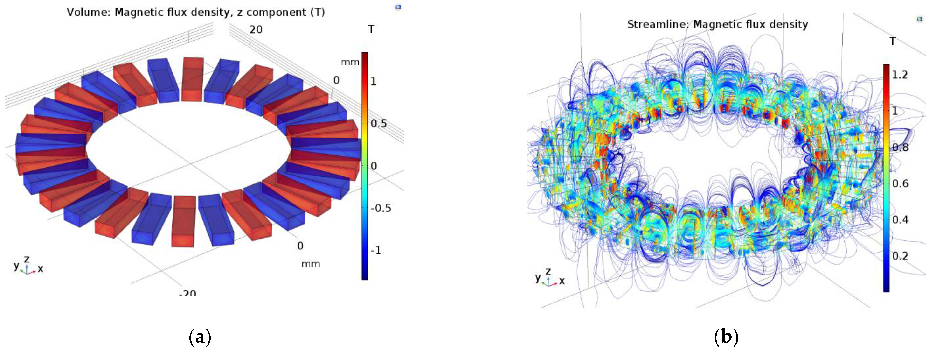
Figure 4a shows an example of a magnetic configuration in which the magnetic flux density propagates through the magnet’s volume in only one direction (z component). However,
Figure 4b presents magnetic flux density lines in the close surroundings of the magnets.
3. Results
COMSOL Multiphysics software allows simulation of physical phenomena using finite element analysis for this purpose. Due to its high level of sophistication and its ability to simulate magnetic fields, it was chosen as the main tool for the following study. Four-disc configurations were used in the simulations, differing in the shape and dimensions of the magnets used, marked as follows: MP—small magnets in the shape of rectangular prisms 10 × 2 × 1.5 mm
3 (length–width–thickness); DP—large magnets in the shape of rectangular prisms 10 × 3 × 1.5 mm
3; MT—small magnets in the shape of trapezoidal prisms 10 × 2.7 × 1.5 × 1.5 mm
3; DT—large magnets in the shape of trapezoidal prisms 10 × 5.3 × 3 × 1.5 mm
3 (length–width 1–width 2–thickness). In the simulations, the rare-earth element sintered NdFeB magnet (neodymium) N38 [
29] was adopted as the magnetic material with a remanence value of 1.21–1.25 T.
Figure 5 shows the configurations studied.
The first stage of the work was to study the magnetic flux density at several selected points around the disc for each configuration. Five lines (arcs) were selected at distances of 16, 18, 20, 22, and 24 mm from the center of the disc (50 mm in diameter). Simulations were carried out at heights equal to 0.25, 0.7, and 1.5 mm above the surface of the disc. Due to the periodicity of the structure, the results presented below were analyzed for an area defined by an angle of 12.85°. This is the area representing 1/28th of the disk (intended for one magnet).
Figure 6 shows the locations (points) where magnetic field simulations were performed for magnetic shields. The area defined by the previously specified angle is also marked.
Figure 7,
Figure 8,
Figure 9 and
Figure 10 show the results for all configurations presented in
Figure 5. In the characteristics, the dashed line indicates the area occupied by the magnet’s geometry, and the dots indicate the area defined by an angle equal to 12.85°.
It can be seen from the above characteristics that, as the distance from the magnet’s surface increases, the value of magnetic flux density decreases. Additionally, this value is not constant along the entire length of the magnets (it changes slightly with the distance from the center of the disc), so average values were determined. For the MP configuration, the highest average value of the magnetic flux density obtained at a distance of 0.25 mm is 386 mT and at a distance of 1.5 mm–122 mT. Very similar values are presented for the MT configuration, with 387 mT and 120 mT, respectively. The distributions for these configurations are also very similar (
Figure 7 and
Figure 9). For the DP configuration (magnets in the shape of rectangular prisms with dimensions of 10 × 3 × 1.5 mm
3), the value of the average magnetic flux density is as follows: 374 mT at a distance of 0.25 mm above the surface and 149 mT at a distance of 1.5 mm. The highest value is observed in the DT configuration, with 389 mT and 160 mT, respectively.
In order to determine the magnetic field distribution over the magnets, many such simulations should be performed for different distances from the center of the disc, and the results should be summed for the entire defined area. Such analysis would be significantly time consuming. Therefore, it was decided to determine approximate values of magnetic flux density for the area on the basis of the above results. For the simulations performed earlier, the value of magnetic flux density occurring over a single area (different colors in
Figure 11 and
Figure 12) was assumed to be constant over a belt with the width of 2 mm (respectively, these are belts with distances from the center of the disc between 15 mm and 17 mm, 17 mm and 19 mm, 19 mm and 21 mm, 21 mm and 23 mm, as well as 23 mm and 25 mm). First, the area defined by the given angle—12.85° (
Figure 11)—was taken for analysis, and then, the area was defined only by the shape of the magnets (
Figure 12).
The summary results are shown in
Table 1.
The value of magnetic flux density over the area defined by the angle of 12.85° is greater than that over the area defined only by the shape of the magnets. In both cases, the smallest value is presented by the MP and MT configurations. On the other hand, the highest value of the magnetic flux density over the given area is represented by the DT configuration, for which the values determined for both areas are also very similar. Finally, the ratio of the magnetic flux density over the area defined by the shape of the magnets to the area defined by the angle of 12.85° was determined. The results are presented in
Table 2. As can be seen from the results presented in
Table 1 and
Table 2, for the same thickness of the magnets, the magnetic field density is proportional to their area. Moreover, the smaller the distance from the target, the greater part of this field is concentrated in the area directly above the surface of the magnet.
The ratio of magnetic flux density over the area defined by the shape of the magnets to the area defined by the angle of 12.85° decreases with the distance increase from the magnet’s disk surface. The DT magnetic configuration is the only instance for which this is not true. As can be observed from the simulations, the configuration of the magnets has a great influence on the shape and value of the magnetic field over the surface of the magnets, in addition to greatly affecting the area surrounding the magnets.
It should be noted that in many papers [
1,
4,
30,
31,
32], authors show that the voltage generated in the coils by a rotating disc with magnets is proportional to the density of magnetic flux. However, in the case of a multilayer coil, the magnetic induction in the various layers of the coil depends on the distance of this layer from the surface of the magnetic disc. It should also be noted that for multilayer coils made of LTCC ceramics, each layer of inductors is separated from the next by 128 µm [
25]. Thus, with eight layers, the difference in distance between the first and eighth layers is approximately equal to 900 µm, i.e., 0.9 mm.
4. Discussion and Conclusions
A magnetic disc is one of the basic components of an electromagnetic microgenerator. When optimizing the device, both components—the coil structure and the magnetic disk—must be considered. The COMSOL Multiphysics program allowed simulation of the magnetic field surrounding the selected magnetic disks. Based on the simulation results, the following conclusions are drawn:
The total magnetic field in a single segment with a magnet is proportional to the area of the magnet;
For magnets in the shape of a rectangular prism, the distances between adjacent magnets increase along with the distance of the analyzed point from the center of the target. At a low height above the disc, the magnetic flux density is approximately constant above the center of the magnet and decreases to zero for approximately 1 mm. For a small rectangle, it is held at this level for about 1 mm in the areas of the magnet closest to the center of the target and 2 mm at the other end of the magnet;
For large magnets in the shape of a rectangular prism, the zero level of magnetic flux density is maintained for about 0–1 mm. There are no sections with zero magnetic induction for magnets in the shape of a trapezoidal prism;
As a result of the rotation of the disc with magnets of various shapes over the spatially set of coils, most uniform changes in the magnetic flux density occur for large magnets in the shape of a trapezoidal prism;
The magnetic flux density decreases non-linearly with increasing distance from the disc with magnets.
Therefore, when designing a disc with magnets, it is necessary to refer to the geometry of the coils so that the surface of the magnets covers as much of the single coil as possible. The presented results of magnetic field distribution are very useful because they show how quickly the magnetic field density in an electromagnetic microgenerator is changed, both depending on the magnetic configuration (their surface area) and the distance from the disc with magnets (very important for the stator made as a multilayer structure with built-in coils).
The coil structure is also a very important parameter. Therefore, further research on electromagnetic generators will focus on coils. They will be simulated on surfaces comparable to those of magnets. The influence of the width of the tracks, the distance between them, and the number of turns on the self- and mutual inductance of a single coil and their set, as well as the series resistance of the coil, will be analyzed. This will allow us to determine the influence of these parameters on the output voltage of the generator and its available power.


