Abstract
This article proposes a model-based method for the detection and phase location of interturn short fault (ISF) in the permanent magnet synchronous generator (PMSG). The simplified mathematical model of PMSG with ISF on dq-axis is established to analyze the fault signature. The current residuals are accurately estimated through Luenberger observer based on the expanded mathematical model of PMSG. In current residuals, the second harmonics are extracted using negative sequence park transform and angular integral filtering to construct the fault detection index. In addition, the unbalance characteristics of three-phase current after ISF can reflect the location of the fault phase, based on which the location indexes are defined. Simulation results for various operating and fault severity conditions primarily validate the effectiveness and robustness of diagnosis method in this paper.
1. Introduction
Permanent magnet synchronous machines (PMSMs) have the advantages of high power density, high efficiency and stability, so it has a wide range of applications in aerospace, electric automobile and new energy power generation [1,2]. In terms of wind power generation, permanent magnet synchronous generators (PMSGs) are currently used extensively compared to doubly fed induction generators (DFIGs), especially in direct-driven power generation systems (PGs) for low weight and volume and the capability of multipole design of PMSGs [3,4,5].
Interturn short faults (ISFs), demagnetization faults, rotor eccentricity and other faults are common faults during the operation of PMSGs, among which ISFs occur most frequently [6]. Due to the damp environment, mechanical vibration, instantaneous overvoltage and other reasons, the winding insulation of PMSGs may be damaged, resulting in the occurrence of ISFs [7]. ISFs will produce large fault current both in the short circuit and fault phase winding, which may cause serious secondary faults such as open circuit, interphase short circuit, and grounding fault [8]. In addition, short-circuited coils will generate magnetomotive force opposite to other coils. The direction of the magnetic field generated by the short-circuited coil is opposite to the direction of the air gap composite magnetic field, which will create the irreversible demagnetization of permanent magnets [9]. Thus, prompt and reliable detection and location algorithms will help in early fault diagnosis to conduct repair and maintenance as soon as possible.
At present, most of the research objects of fault detection technology, at home and abroad, are induction motors (IMs). Due to the relatively short time of appearance, the fault detection technology of PMSMs or PMSGs is still in the development stage. The existing fault detection methods for PMSMs can be roughly divided into the following three types: the method based on analytical model; the method based on knowledge; and the method based on signal processing [10,11]. The first method constructs an accurate mathematical model of the motor through the logical relationships between the parameters of the system, so the model can predict the output under healthy conditions. This method judges the occurrence of the fault by comparing the residuals between the predicted output and the actual output of the motor [12]. The main advantage of this approach is that no additional hardware is required to implement fault detection and isolation algorithms. In reference [13], an efficient, simplified physical faulty model considering the disposition of coils under the same or different pole-pair is proposed, which can simulate different types of stator faults. In reference [14], model predictive control (MPC) is used in the PMSM control system and detection is acquired by analyzing the dc component and the second harmonic in the cost function.
The knowledge-based method can be divided into model-based reasoning, neural network based and fuzzy logic based fault diagnosis methods, based on different sources of knowledge learning [15,16]. Common diagnosis methods include artificial neural network, fuzzy logic diagnosis, expert system and information fusion diagnosis, etc. [17]. The method avoids the high dependence on the machine model, and can introduce many aspects of motor information, which opens up a new path for research of fault detection. In reference [18], a diagnostic system based on convolutional neural network (CNN) is proposed to detect the PM damages using raw phase current signals. However, the complexity of the algorithm reduces the possibility of real-time diagnosis. To detect and locate the open-circuit of PWM-VSI in the PMSM drive, the fuzzy logic method is used to process fault diagnosis variables from the average current Park’s vector in reference [19], but the problem of poor self-learning still exists. In reference [20], the vibrations and currents of the fault machine are calculated using a multidimensional diagnosis methodology, and support vector machine (SVM) is used to classify single and combined fault scenarios under different speed and torque conditions.
The signal processing method collects the voltage, current, output torque, back electromotive force (EMF) and other signals of the fault machine, then uses various signal processing methods to extract and analyze the time-frequency domain characteristics of the fault signal for fault diagnosis [21,22]. Common signal processing methods include fast Fourier transform (FFT), Hilbert-Huang transform (HHT), wavelet transform (WT) and empirical mode decomposition (EMD). The method does not need accurate motor analytical model and related parameters, and has strong adaptability, which is a mature and widely used method in motor fault detection. In reference [23], HF rotating square-waveform voltages are injected to detect and classify the turn fault and high-resistance connection (HRC) fault of PMSM, by extracting HF currents consisting of fault characteristics. Reference [24] proposes a diagnosis algorithm based on discrete wavelet transform (DWT) and SVM, and designs an adaptive filter to address the problem of harmonic removal. Reference [25] uses EMD energy entropy and normalized average current to diagnose open-circuit faults of one or more phases in the PMSM drive circuit, which can also be used for interturn fault detection.
In addition, the fast location of the fault phase ensures the efficiency and accuracy of the overall fault diagnosis algorithm of PMSMs. Common fault location algorithms, on the one hand, use the amplitude and phase difference of fault phase current or voltage as the diagnosis basis [26], or acquire the waveform distortion of the magnetomotive force under fault conditions, which require additional equipment investment [27]. Thus, there are still a lack of clear indexes for fault location under variable conditions and the accuracy of the location algorithm needs to be further improved.
The accuracy of residual-based fault diagnosis methods depends on how accurately the residual is measured. The residuals (current, voltage, EMF) can be obtained by building an accurate model of the normal machine, which can be established from lumped parameters and finite element (FE) analysis [28], or using a virtual observer such as the Luenberger observer, sliding mode observer (SMO) and extended state observer. Since data in a healthy state are generally obtained from steady-state conditions, the effects of transient speed and load conditions on the detection performance cannot be neglected. However, the measurement method based on a virtual observer can be applied to variable operating conditions without additional equipment investment.
The paper proposes a new detection and location strategy for ISF in PMSGs based on extracting and analyzing the negative sequence residuals. The current residuals are accurately measured by the Luenberger observer. The defined fault diagnosis and phase location indexes can be extracted from the residuals through negative sequence park transform and angular integral filtering. The indexes have good robustness to speed and load fluctuation, which can adapt to the speed variations of wind turbine under the maximum power point tracking (MPPT) or limited power state.
The paper consists of five essential parts. In Section 2, a simplified ISF model of PMSG on dq-axis is established to analyze the fault components on dq-axis. In Section 3, the Luenberger observer based on expanded mathematical model on dq-axis is designed to accurately measure current residuals under fault conditions. Section 4 defines the fault detection and fault phase location indexes, which consider speed and load fluctuation during operation of PMSG. Finally, simulation results in Matlab/Simulink are given in Section 5.
2. Mathematical Model of PMSG with ISF
2.1. Wind Turbine Aerodynamic Model
According to Baez theory and aerodynamics, the mechanical power Pw captured by wind turbines from wind energy are expressed as [29]:
where ρ is the air density, R is the wind turbine radius, λ = ωmR/v is the tip speed ratio, v is the wind speed, ωm is the mechanical speed of the wind turbine; Cp is the power coefficient, β is the blade pitch.
Figure 1 shows the wind turbine power-rotor speed characteristic curves at different wind speeds, the maximum power points (MPPs) under different wind speeds forms the optimal power curve. PMSGs usually operates under maximum power point tracking (MPPT) control, where there is a optimal value λopt at which the PMSGs can extracts the maximum power Pw_opt from wind given by:
where Cpmax is the maximum power coefficient, k is the optimal power constant, which is only related to the characteristic parameters of the wind turbine. Accordingly, the optimal torque at MPPs is expressed as:
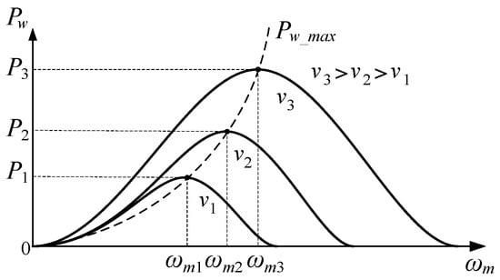
Figure 1.
Wind turbine power-rotor speed characteristic curves at different wind speeds.
2.2. Modeling of the PMSG with ISF
Considering there is only one branch in each phase winding, the electrical model of PMSG with ISF in phase a is shown in Figure 2. The faulty winding a is divided into the healthy and faulted parts. The faulted part is represented by a winding with resistance Raf, inductance Laf, and back EMF eaf, and the current flow through it is defined as faulted current iaf. The contract resistance in shorted path is defined as Rf, with the short-circuit current if flowing through it. The ratio of number of turns in faulted winding to the total number of turns per phase is defined as μ, which ranges from 0 to 1. The ratio μ and Rf collectively represent the fault severity of the ISF. Under ideal conditions, the resistance and back EMF can be considered proportional to number of turns, and the inductance is proportional to the square of turns. Thus, the parameters both in the healthy and faulted parts can be calculated accordingly.

Figure 2.
Electrical model of PMSG with ISF in phase a.
From reference [30], the mathematical model of PMSG with ISF can be expressed in (4), where Rs is stator resistance, θe is electrical angle. L and M are self and mutual inductance of stator winding respectively, λPM is the PM flux linkages.
Considering the voltage in the faulty phase can be written as:
The current and voltage of faulted portion have relations as follows:
Using (5) and (6) in (4), the three-phase voltages equations under turn fault conditions can be rewritten as:
By Park transformation, the voltage equations of PMSG with ISF in dq coordinate can be written as:
where ωe is the electrical angular speed, udf and uqf are dq-axis voltages in ISF condition, id and iq are dq-axis currents in normal condition, and Ld and Lq are dq-axis inductance. The angle θe will be replaced with (θe − 2π/3) or (θe + 2π/3) when ISF occurs in phase b or c.
Rearrange the voltage Equation (8) as:
where idf and iqf are dq-axis current in ISF situation, which can be written as:
Equation (9) has the same form as the normal voltage equations. It means if the same voltage udf and uqf in (8) are applied in the normal model conditions, the fault current with ISF can be extracted and expressed in (10). The Δid and Δiq are defined as current residuals, whose magnitude only depends on μ and if. Since the residuals equal to zero under normal conditions and can indicate the severity of the ISF, it is a stable and robust signature for ISF detection.
From reference [31], the electromagnetic torque of the PMSG with ISF is expressed as:
where eabc are the back electromotive force, the mechanical torque of the wind turbine is the load torque of PMSG, so the mechanical part of PMSG can be described as:
where J is the rotor inertia, B is the damping coefficient, which characterizes the combined viscous friction of rotor and load.
3. Estimation of Current Residuals
3.1. Design of State Observer
As expressed in (10), the current residuals can be obtained by measuring the difference between currents in ISF and healthy conditions. However, the healthy model needs to be accurate enough to meet diagnostic needs, and this measuring method need to store and invoke voltage and current data under different operating conditions. In contrast, the flexibility of the virtual observer and the need for no additional equipment investment make up for this defect. The paper use the Luenberger observer for the estimation of current residuals for its dynamic response performance and estimation accuracy.
According to (9) and (10), the current residuals can be defined as state variables, and the expanded mathematical model of PMSG with ISF can be written as:
where
and are the state variables, are the output variables, are the control variables, A is the state matrix, B is the input matrix, and C is the output matrix.
In order to measure the current residuals, the classical Luenberger observer can be designed as:
where superscript ‘^’ indicates the estimated value. is the observation matrix. Figure 3 shows the structure diagram of the Luenberger observer.
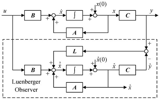
Figure 3.
Structure diagram of the Luenberger observer.
The Luenberger observer reflects the error between the observation state and the actual state to the observation output through the observation matrix L. Therefore, the selection of the parameter L will affect the convergence and accuracy of the observer.
3.2. Stability Aanlysis
As mentioned above, the parameter design of observation matrix L is crucial, to simplify the parameter design process, it is set that l2 = l3 = l6 = l7 = 0. The state error equation of the observer can be obtained by making a difference between Equations (13) and (17) above:
where (A − LC) is the system state matrix of the observer, whose eigenvalue is called system poles of the observer. When the poles of the system are all located in the left half plane of the s-domain, or the real components of the eigenvalues of state matrix (A − LC) are all negative, the system response will decay and tend to be stable. The characteristic equation for (A − LC) can be written as:
where
For the observer system, the commonly used stability judgment methods include Routh criterion, Hurwitz criterion, Nyquist criterion and Root Locus method, etc. The Hurwitz criterion is more suitable for the stability analysis of the fourth order system for its simple rules and convenient use. Therefore, the Hurwitz determinant of characteristic Equation (21) can be written as:
According to the Hurwitz criterion, the Luenberger observer of PMSG designed above has global stability only when the principal determinant of each order of D4 is greater than zero. In order to ensure that the observer system has a higher bandwidth than the original system without observer, the larger the parameters of the L are, the better the dynamic characteristics of the observer. However, the parameters of L are firstly limited by the saturation characteristics of the devices in actual system. Secondly, there are usually interference and measurement noise in the measured output y of the actual system. Excessive parameter setting will amplify system interference and noise. Considering the level of noise measured by the actual system, in order to avoid the pulsation caused by amplified noise, the observer poles are generally 2~10 times of the original system poles [32]. How to select the gain parameters according to the working conditions is still a key issue.
4. Detection and Location Strategy of ISF
4.1. Fault Detection
Without considering high-order harmonics, the short-circuit current if can be expressed as:
where If and θF are the amplitude and initial phase angle of short-circuit current. The amplitude is mainly affected by shorted turn ratio μ and fault resistance Rf, but also related to speed and load condition of PMSG. While the phase angle θF is associate with the location of the fault, which is synchronized with the initial phase angle of the fault phase.
By substituting (22) into (10), it has:
It can be concluded from (23) that the current residuals on dq-axis contain dc components and second harmonics. The amplitudes of both are related to the amplitude of short-circuit current and shorted turn ratio, both can be used as index parameters to characterize the severity of ISF. However, the dc component is also affected by the θF. When the θF approaches a certain value, the dc component residuals on axis d or q may decrease to zero, thus affecting fault judgment. In addition, when the actual parameters of the generator do not match the theoretical parameters, or when the sudden change of the speed or load torque of the motor causes the offset of the fault angle, these will introduce the dc component into the current differential Equation (9) without affecting the higher harmonic component. Therefore, this paper selects the second harmonics of current residuals on dq-axis to construct the fault index.
From reference [33], the amplitude of short-circuit current If is approximately proportional to the speed of the motor. Therefore, the above-mentioned index FIsum will fluctuate when the motor speed changes or the outside wind speed changes for wind turbines, which is not conducive to the determination of the fault detection threshold. In order to eliminate the influence of the speed on the fault index, the fault index need to be reconstructed into the following form:
The above index is only proportional to the ratio μ, but not to other factors such as speed. The construction of FI needs to extract the second harmonics of current residuals. A common frequency domain analysis algorithm, such as FFT, HHT and WT, decompose and reconstruct signals in frequency domain or time-frequency domain. However, these algorithms need to track the frequency of the motor in real time, which will fluctuate under ISF, thus resulting in the final measurement bias. To avoid this, extraction of second harmonic residuals can be indirectly accomplished by negative sequence Park transformation as follows:
where superscript ‘n’ indicates the value in negative sequence. Through the above transformation, the second harmonics of the current residuals in the positive sequence coordinates are the dc components in the negative sequence coordinates. Thus, only the high-order harmonic components other than the dc component need to be filtered out, which does not need to reselect the cut-off frequency of filters due to the change of motor operating frequency during ISF.
Traditional researches generally employ low pass filter or notch filter to filter out high-order harmonic components and preserve dc components. However, when the operating frequency changes, the parameters of the filter need to be adjusted accordingly, resulting in the detection error. To solve this, the paper presents a method based on angle integral filter to accurately measure the dc components of negative sequence current residuals, which can be incorporated into the original measurement algorithm. The principle of angular integral filtering can be expressed as:
where θn is a complete electrical angle cycle, generally 2π. Therefore, the above fault index for ISF can be redefined as:
4.2. Fault Location
When the ISF occurs in PMSGs, the three-phase current will no longer maintain phase symmetry, and the phase angle difference between non-fault phases will decrease with the severity of fault. Figure 4 shows the phase angle change with ISF in phase a.

Figure 4.
Phase angle changes with ISF in phase a.
Under the premise of ignoring the influence of higher harmonics, the stator three-phase current of PMSG can be expressed as:
where Ij and θj (j = a, b, c) are the amplitude and initial phase of phase current, respectively. The phase angle differences between phase currents can be defined as:
When the PMSG operates normally, there is θab = θbc = θac = π/3. While the phase angle differences between the fault phase and the non-fault phases will increase (>π/3), and the phase angle difference between the non-fault phases will decrease (<π/3) when ISF occurs. Based on the above signature, the fault phase location indexes can be defined as follows:
The theoretical value of fault location indexes when ISF occurs in different phases is shown in Table 1. There is a clear boundary between the location indexes of the fault phase and non-fault phases, which can be used to locate the fault phase. Under the same operating condition, the degree of deviation of the location indexes from 1 can reflect the severity of the fault to some extent.

Table 1.
Theoretical value of fault location indexes with ISF.
For phase angle measurement of three-phase current, the currents can be projected to a rotating coordinate system, which can be expressed as:
where j = a, b, c. Subscripts ‘2nd’ and ‘dc’ are the second harmonic and dc component respectively. According to Equation (32), the dc component in the rotating coordinate systems contains the initial phase angle of the three-phase current. Therefore, the angular integral filtering method mentioned above can be used to extract the dc components first, and then the reconstruction can be carried out as follows:
4.3. Overall Process of Fault Detection and Location
The overall process of ISF detection and location in PMSG in this paper is shown in Figure 5. Firstly, the residual currents on dq-axis in the ISF state is observed by the Luenberger observer. Secondly, the dc components in the negative sequence current residuals are extracted by negative sequence Park transformation and angular integral filter to construct fault detection index, and the initial phase angle of three-phase currents are calculated by the method of rotating coordinate projection, on which the fault location indexes are constructed. Finally, the measured parameters are compared with the normal conditions to determine whether the ISF occurs in PMSG, thus send out alarm signal or trip the circuit breaker according to the severity of the fault.
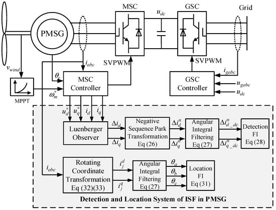
Figure 5.
Overall process of ISF detection and location in PMSG.
5. Simulation Verification
In order to verify the effectiveness and rationality of the ISF detection and location strategy proposed in this paper, the ISF model of PMSG is built in Matlab/Simulink for simulation testing. The parameters of PMSG used in the simulation are shown in Table 2. Before the simulation time t = 1.3 s, the PMSG is in a healthy state. When t = 1.3 s, the ISF occurs in phase a by closing the breaker of the short circuit. The short circuit parameters are set to μ = 0.15, Rf = 0.002.
Table 2.
Parameters of the PMSG based wind power system.
5.1. ISF Detection under Steady Wind Speed
The simulated wind speed vwind is set as 10 m/s. Figure 6 shows the simulation waveforms of three-phase current, rotation speed and electromagnetic torque of the PMSG in healthy and failure states. The three-phase current will lose symmetry after ISF, and harmonic components appear in the speed and electromagnetic torque, which conforms to the basic characteristics of the fault.

Figure 6.
Simulation results. (a) Three-phase current of stator; (b) speed; (c) electromagnetic torque.
The waveforms of current residuals on dq-axis are shown in Figure 7a–c is the spectrum of current residuals after the fault. Under normal conditions, the current residuals are almost equal to zero, so the spectrum analysis of the signal before the fault is not very meaningful. After the fault, obvious dc component and second harmonics appear in the residuals. The second harmonic on d-axis and q-axis have almost the same amplitude, while the difference between dc components is mainly related to the fault location, which is consistent with the theoretical analysis result of Equation (23) above.

Figure 7.
Simulation results of current residuals. (a) d-axis current residual; (b) q-axis current residual; (c) spectrum of current residuals after ISF.
Figure 8 shows the simulation results of fault detection and phase location indexes under health and fault conditions. When the PMSG is in a healthy state, the fault detection index is close to 0, and the three-phase location indexes are all close to 1. After the ISF occurs, the detection index mutates and stabilizes to 1.044 within 0.05 s. The location indexes show a difference after 0.1 s, ka > 1, and it is significantly greater than indexes of other two phases, which corresponds to the occurrence of ISF in phase a.

Figure 8.
Simulation results of fault detection and fault location indexes. (a) Fault detection index; (b) fault phase location indexes.
Considering that the interturn fault are not handled in time, which may lead to further failures, it is necessary to study the universality of fault indexes in continuous state. The degree of failure is mainly determined by the shorted turn ratio μ and fault resistance Rf. Figure 9 shows the influence of different μ and Rf on fault indexes under continuous operation state. In Figure 9a,b, the fault resistance Rf is set to 0.02, the ratio μ increases by 0.05 every 0.5 s after 1 s. With the increase of shorted turn ratio μ, both detection index FI and fault phase location indexes kabc increase proportionally. In Figure 9c,d, the shorted turn ratio μ is set to 0.15, the fault resistance Rf rises from 0.005 to 0.04. As the fault resistance Rf increases, the detection index FI and fault phase location indexes kabc decrease inversely. When Rf > 0.03, kabc has almost become stable with little change. Therefore, the proposed fault detection index and fault phase location indexes can reflect the severity of the ISF.

Figure 9.
Fault detection index and fault phase location indexes under different fault severity. (a) Detection index with different μ when Rf = 0.02; (b) location indexes with different μ when Rf = 0.02; (c) detection index with different Rf when μ = 0.15; (d) location indexes with different Rf when μ = 0.15.
Figure 10 shows the changes of detection index and location index under different wind speeds. Since the wind generator work under MPPT mode, different wind speeds mean that the PMSG will track the maximum power point at different optimal speeds. In Figure 10a,c, the changes of wind speed has little impact on the detection index FI under the same fault severity. Therefore, the threshold of fault detection index is almost universal for different working wind speeds. In Figure 10b,d, the location index of fault phase ka decreases with the increase of wind speed, but the decrease is not large, and is obviously larger than that of healthy state, so the indexes are still effective in the location of the ISF.

Figure 10.
Fault detection index and fault phase location index under different wind speeds. (a) Detection index FI with different μ; (b) location index ka with different μ; (c) detection index FI with different Rf; (d) location index ka with different Rf.
5.2. ISF Detection under Variable Wind Speed
In the above, the fault detection is carried out under the steady state of a specific wind speed, while the PMSG mostly works under continuously changing wind speed, so the following will discuss the ISF detection under variable wind speed. Figure 11a shows the stepped wind speed input. The optimum, and actual speed, of PMSG are shown in Figure 11b. Under MPPT control mode, the speed of PMSG can still track the basic trajectory of the optimum speed, but there is obvious fluctuation caused by ISF. In Figure 11c, the fault detection index of the same fault severity is almost the same at different wind speeds. At the moment of step change of wind speed, the index value will fluctuate, but the fluctuation is limited, which needs to be considered when selecting the fault threshold. However, the fault phase location index may change suddenly when the wind speed surges, and the indexes of non-fault phases may be greater than 1, thus affecting the location results. Therefore, the fault phase location can be carried out after the fault detection index is stable.

Figure 11.
Fault detection results under stepped wind speed. (a) Stepped wind speed; (b) pptimum and actual speeds of PMSG; (c) fault detection index; (d) fault phase location indexes.
Under the stepped wind speed in Figure 11a, the fault detection index curves of different fault severity are shown in Figure 12. From the simulation results, the sudden change of the wind speed will cause the fluctuation of detection indexes under different fault severity, but the overall trend is stable, which will not have a great impact on the final fault diagnosis.

Figure 12.
Fault detection results under stepped wind speed with different μ.
On the basis of above simulation under stepped wind speed, when the wind generator operates at random wind speed as shown in Figure 13a, the simulation results are shown in Figure 13. The speed and electromagnetic torque of the PMSG have obvious harmonics after ISF. Under the continuously changing wind speed, the detection index cannot reach a relatively stable state due to the measurement error caused by the low frequency of the PMSG, but it is obviously larger than the index curve under the healthy state, so it is still effective for ISF diagnosis.

Figure 13.
Fault detection results at random wind speed. (a) Random wind speed; (b) optimum and actual speeds of PMSG; (c) electromagnetic torque; (d) fault detection index.
Under the random wind speed in Figure 13a, the fault detection index curves of different fault severity are shown in Figure 14. Compared with stepped wind speed, the fluctuation of detection index is more intense with the deepening of fault severity, but there are still clear boundaries between different curves. If subsequent fault severity prediction is required after diagnosis, it can be distinguished by calculating the energy spectrum or power spectrum of the curves.

Figure 14.
Fault detection results at random wind speed with different μ.
6. Conclusions
A robust fault detection and location strategy for ISF in PMSGs based on negative sequence current residuals is presented in this paper. The proposed method utilizes the second harmonics in the residuals as a reliable fault signature rather than the dc components since the dc components are not only related to the severity of the ISF, but also affected by the short circuit location and errors of the motor parameters. The current residuals on dq-axis are acquired by the Luenberger observer based on the expanded mathematical model of PMSG. The second harmonics are extracted through negative sequence park transform and angular integral filtering equivalently. By reconstructing the negative sequence current residuals, the defined fault detection index has great robustness to the normal speed fluctuation of wind generator. In addition, the unbalance characteristics of three-phase current after ISF can reflect the location of the fault phase, which is the basis for the definition of location indexes. However, there are mutations in location indexes, so the location of fault phase can be done after detection index is stable. The extensive simulation results in Matlab/Simulink validated the effectiveness and stability of fault detection and fault phase location method proposed in this paper.
Author Contributions
Conceptualization, T.W. and S.C.; methodology, W.D. and X.L. (Xindong Li); software, W.D.; validation, Y.Z., X.L. (Xiaobao Liu) and X.L. (Xindong Li).; formal analysis, S.C.; investigation, T.W.; resources, T.W.; data curation, T.W. and W.D.; writing—original draft preparation, S.C.; writing—review and editing, S.C.; visualization, X.L. (Xiaobao Liu); supervision, T.W.; project administration, T.W.; funding acquisition, T.W. All authors have read and agreed to the published version of the manuscript.
Funding
This work was supported by State Key Laboratory of Smart Grid Protection and Control, Nari Group Corporation, Nanjing, Jiangsu, 211106, China. (Project No. SGNR0000KJJS2200310).
Data Availability Statement
Not applicable.
Conflicts of Interest
The authors declare no conflict of interest.
References
- Lee, H.; Jeong, H.; Kim, S.W. Diagnosis of Interturn Short-Circuit Fault in PMSM by Residual Voltage Analysis. In Proceedings of the 2018 International Symposium on Power Electronics, Electrical Drives, Automation and Motion (SPEEDAM), Amalfi, Italy, 20–22 June 2018; pp. 160–164. [Google Scholar]
- Moosavi, S.S.; Djerdir, A.; Amirat, Y.; Khaburi, D.A. Demagnetization fault diagnosis in permanent magnet synchronous motors: A review of the state-of-the-art. J. Magn. Magn. Mater. 2015, 391, 203–212. [Google Scholar] [CrossRef]
- Yao, J.; Pei, J.; Xu, D.; Liu, R.; Wang, X.; Wang, C.; Li, Y. Coordinated control of a hybrid wind farm with DFIG-based and PMSG-based wind power generation systems under asymmetrical grid faults. Renew. Energy 2018, 127, 613–629. [Google Scholar] [CrossRef]
- Yao, J.; Liu, R.; Zhou, T.; Hu, W.; Chen, Z. Coordinated control strategy for hybrid wind farms with DFIG-based and PMSG-based wind farms during network unbalance. Renew. Energy 2017, 105, 748–763. [Google Scholar] [CrossRef]
- Yaramasu, V.; Wu, B.; Alepuz, S.; Kouro, S. Predictive Control for Low-Voltage Ride-Through Enhancement of Three-Level-Boost and NPC-Converter-Based PMSG Wind Turbine. IEEE Trans. Ind. Electron. 2014, 61, 6832–6843. [Google Scholar] [CrossRef]
- Zafarani, M.; Bostanci, E.; Qi, Y.; Goktas, T.; Akin, B. Interturn Short-Circuit Faults in Permanent Magnet Synchronous Machines: An Extended Review and Comprehensive Analysis. IEEE J. Emerg. Sel. Top. Power Electron. 2018, 6, 2173–2191. [Google Scholar] [CrossRef]
- Cintron-Rivera, J.G.; Foster, S.N.; Strangas, E.G. Mitigation of turn-to-turn faults in fault tolerant permanent magnet synchronous motors. IEEE Trans. Energy Convers. 2015, 30, 465–475. [Google Scholar] [CrossRef]
- Gandhi, A.; Corrigan, T.; Parsa, L. Recent Advances in Modeling and Online Detection of Stator Interturn Faults in Electrical Motors. IEEE Trans. Ind. Electron. 2011, 58, 1564–1575. [Google Scholar] [CrossRef]
- Moon, S.; Lee, J.; Jeong, H.; Kim, S.W. Demagnetization Fault Diagnosis of a PMSM Based on Structure Analysis of Motor Inductance. IEEE Trans. Ind. Electron. 2016, 63, 3795–3803. [Google Scholar] [CrossRef]
- Chen, Y.; Liang, S.; Li, W.; Liang, H.; Wang, C. Faults and Diagnosis Methods of Permanent Magnet Synchronous Motors: A Review. Appl. Sci. 2019, 9, 2116. [Google Scholar] [CrossRef]
- Bhuiyan, E.A.; Akhand, M.M.A.; Das, S.K.; AliMd, F.; Tasneem, Z.; Islam, Md.R.; Saha, D.K.; Badal, F.R.; Ahamed, Md.H.; Moyeen, S.I. A Survey on Fault Diagnosis and Fault Tolerant Methodologies for Permanent Magnet Synchronous Machines. Int. J. Autom. Comput. 2020, 17, 763–787. [Google Scholar] [CrossRef]
- Qian, H.; Guo, H.; Ding, X. Modeling and Analysis of Interturn Short Fault in Permanent Magnet Synchronous Motors With Multistrands Windings. IEEE Trans. Power Electron. 2016, 31, 2496–2509. [Google Scholar] [CrossRef]
- Ben Khader Bouzid, M.; Champenois, G.; Maalaoui, A.; Tnani, S. Efficient Simplified Physical Faulty Model of a Permanent Magnet Synchronous Generator Dedicated to the Stator Fault Diagnosis Part I: Faulty Model Conception. IEEE Trans. Ind. Appl. 2017, 53, 2752–2761. [Google Scholar] [CrossRef]
- Hang, J.; Zhang, J.; Xia, M.; Ding, S.; Hua, W. Interturn Fault Diagnosis for Model-Predictive-Controlled-PMSM Based on Cost Function and Wavelet Transform. IEEE Trans. Power Electron. 2020, 35, 6405–6418. [Google Scholar] [CrossRef]
- Yang, Z.; Wang, Y.; Lv, J. Survey of modern Fault Diagnosis methods in networks. In Proceedings of the 2012 International Conference on Systems and Informatics (ICSAI2012), Yantai, China, 19–20 May 2012; pp. 1640–1643. [Google Scholar]
- Fu, X. Statistical machine learning model for capacitor planning considering uncertainties in photovoltaic power. Prot. Control Mod. Power Syst. 2022, 7, 51–63. [Google Scholar] [CrossRef]
- Tang, S.; Yuan, S.; Zhu, Y. Deep Learning-Based Intelligent Fault Diagnosis Methods Toward Rotating Machinery. IEEE Access 2020, 8, 9335–9346. [Google Scholar] [CrossRef]
- Skowron, M.; Orlowska-Kowalska, T.; Kowalski, C.T. Detection of Permanent Magnet Damage of PMSM Drive Based on Direct Analysis of the Stator Phase Currents Using Convolutional Neural Network. IEEE Trans. Ind. Electron. 2022, 69, 13665–13675. [Google Scholar] [CrossRef]
- Yan, H.; Xu, Y.; Cai, F.; Zhang, H.; Zhao, W.; Gerada, C. PWM-VSI Fault Diagnosis for a PMSM Drive Based on the Fuzzy Logic Approach. IEEE Trans. Power Electron. 2019, 34, 759–768. [Google Scholar] [CrossRef]
- Delgado, M.; García, A.; Ortega, J.A.; Cárdenas, J.J.; Romeral, L. Multidimensional intelligent diagnosis system based on Support Vector Machine Classifier. In Proceedings of the 2011 IEEE International Symposium on Industrial Electronics, Gdansk, Poland, 27–30 June 2011; pp. 2124–2131. [Google Scholar]
- Haje Obeid, N.; Battiston, A.; Boileau, T.; Nahid-Mobarakeh, B. Early Intermittent Interturn Fault Detection and Localization for a Permanent Magnet Synchronous Motor of Electrical Vehicles Using Wavelet Transform. IEEE Trans. Transp. Electrif. 2017, 3, 694–702. [Google Scholar] [CrossRef]
- Wang, B.; Wang, J.; Griffo, A.; Sen, B. Stator Turn Fault Detection by Second Harmonic in Instantaneous Power for a Triple-Redundant Fault-Tolerant PM Drive. IEEE Trans. Ind. Electron. 2018, 65, 7279–7289. [Google Scholar] [CrossRef]
- Hu, R.; Wang, J.; Mills, A.R.; Chong, E.; Sun, Z. High-Frequency Voltage Injection Based Stator Interturn Fault Detection in Permanent Magnet Machines. IEEE Trans. Power Electron. 2021, 36, 785–794. [Google Scholar] [CrossRef]
- Heydarzadeh, M.; Zafarani, M.; Akin, B.; Nourani, M. Automatic fault diagnosis in PMSM using adaptive filtering and wavelet transform. In Proceedings of the 2017 IEEE International Electric Machines and Drives Conference (IEMDC), Miami, FL, USA, 21–24 May 2017; pp. 1–7. [Google Scholar]
- Wu, Y.; Zhang, Z.; Li, Y.; Sun, Q. Open-Circuit Fault Diagnosis of Six-Phase Permanent Magnet Synchronous Motor Drive System Based on Empirical Mode Decomposition Energy Entropy. IEEE Access 2021, 9, 91137–91147. [Google Scholar] [CrossRef]
- He, S.; Shen, X.; Jiang, Z. Detection and Location of Stator Winding Interturn Fault at Different Slots of DFIG. IEEE Access 2019, 7, 89342–89353. [Google Scholar] [CrossRef]
- Yin, Z.; Sui, Y.; Zheng, P.; Yang, S.; Zheng, Z.; Huang, J. Short-Circuit Fault-Tolerant Control Without Constraint on the D-Axis Armature Magnetomotive Force for Five-Phase PMSM. IEEE Trans. Ind. Electron. 2022, 69, 4472–4483. [Google Scholar] [CrossRef]
- Moon, S.; Jeong, H.; Lee, H.; Kim, S.W. Interturn Short Fault Diagnosis in a PMSM by Voltage and Current Residual Analysis With the Faulty Winding Model. IEEE Trans. Energy Convers. 2018, 33, 190–198. [Google Scholar] [CrossRef]
- Yin, X.X.; Lin, Y.G.; Li, W.; Liu, H.W.; Gu, Y.J. Fuzzy-Logic Sliding-Mode Control Strategy for Extracting Maximum Wind Power. IEEE Trans. Energy Convers. 2015, 30, 1267–1278. [Google Scholar] [CrossRef]
- Romeral, L.; Urresty, J.C.; Riba Ruiz, J.R.; Garcia Espinosa, A. Modeling of Surface-Mounted Permanent Magnet Synchronous Motors with Stator Winding Interturn Faults. IEEE Trans. Ind. Electron. 2011, 5, 1576–1585. [Google Scholar] [CrossRef]
- Otava, L.; Buchta, L. PMSM stator winding faults modelling and measurement. In Proceedings of the 2015 7th International Congress on Ultra Modern Telecommunications and Control Systems and Workshops (ICUMT), Brno, Czech Republic, 6–8 October 2015; pp. 138–143. [Google Scholar]
- Andersson, A.; Thiringer, T. Motion Sensorless IPMSM Control Using Linear Moving Horizon Estimation with Luenberger Observer State Feedback. IEEE Trans. Transp. Electrif. 2018, 4, 464–473. [Google Scholar] [CrossRef]
- Gurusamy, V.; Bostanci, E.; Li, C.; Qi, Y.; Akin, B. A Stray Magnetic Flux-Based Robust Diagnosis Method for Detection and Location of Interturn Short Circuit Fault in PMSM. IEEE Trans. Instrum. Meas. 2021, 70, 1–11. [Google Scholar] [CrossRef]


Publisher’s Note: MDPI stays neutral with regard to jurisdictional claims in published maps and institutional affiliations. |
© 2022 by the authors. Licensee MDPI, Basel, Switzerland. This article is an open access article distributed under the terms and conditions of the Creative Commons Attribution (CC BY) license (https://creativecommons.org/licenses/by/4.0/).