Optimal Control of the Diesel–Electric Propulsion in a Ship with PMSM

Abstract

The article presents and compares two different control methods for a permanent magnet synchronous motor (PMSM) for diesel–electric ship propulsion. The main focus of the article is on control optimization, which allows improving energy efficiency by reducing reactive power in the mechatronic propulsion system. The first method consists in modifying the commonly used field-oriented control (FOC) strategy to ensure zero reactive power in the inverter–PMSM system. Since a characteristic of ship propulsion systems, unlike those used on land, is the step load on the propulsion motor, the system’s performance in dynamic states is particularly important. Unfortunately, control strategies based on FOC do not take into account the dynamics of the system, since they apply only to steady states. Therefore, the authors of this paper, based on control theory methods, proposed an approach that also optimizes control in dynamic states, while minimizing reactive power in the steady state. The analytical studies were confirmed in simulation studies using the MATLAB Simulink package.

1. Introduction

Due to the fact that approximately 80% of world trade is carried out by sea [1], maritime organizations and designers of ship systems are looking for solutions limiting the negative effects of ships on the environment. In this context, the International Maritime Organization (IMO) has presented rigorous regulations concerning the design of ship systems by introducing the Energy Efficiency Design Index (EEDI) [2,3,4,5]. The introduced regulations pose a great challenge for engineers, who (at every stage of ship design) are looking for solutions to improve the EEDI by applying new technologies or increasing the efficiency of currently applied systems.

The most frequently used ship propulsion system is an internal combustion engine mechanically connected to a propeller with a constant pitch or with a variable pitch (less frequently). The main disadvantage of internal combustion engines is their low efficiency—especially at low engine loads. The typically used low-speed diesel engines show up to 50% efficiency at optimal load [6]. It should be stressed that ships with combustion engines and fixed propellers have maneuvering limitations.

Nowadays, this propulsion is a solution commonly used for ships, which move at design speed [7] for most of their operation.

For ships that require high flexibility of the propulsion system, e.g., cruise ships, ferries, pleasure vessels, and offshore ships (anchor handling tug vessels, accommodation ships, supply vessels), thanks to the development of power electronics technologies, diesel–electric propulsion systems have been an alternative solution to internal combustion engines. In addition, this drive is characterized, among other things, by high reliability and overall cost reduction (investment and exploitation) [7,8].

The traditionally used power generation system and the ship propulsion in the diesel–electric system are presented in Figure 1 [7,9,10,11,12,13].

Compared to the propulsion of a ship with an internal combustion engine, the efficiency of the diesel–electric propulsion at full load is lower due to additional losses of the power electronics system and the electric motor (approximately 4% [7,14]). However, with a reduced load, the efficiency of the diesel–electric system is greater. This is due to the operation of a smaller number of generating sets, and thus the optimal operation of the remaining generating sets. In ships with AC grids, all generating units operate at a constant speed in order to ensure the stability and safety of the ship’s power grid.

Increasing the efficiency of the diesel–electric system and therefore increasing the efficiency of the drive can be achieved by using the topology shown in Figure 2.

The ship propulsion system with optimized operation of generator propulsion engines is also known (Figure 2) [7,15,16,17,18,19,20].

In the DC grid, it is possible to optimize the operation of generator propulsion engines. Each diesel engine can run independently in the DC grid at optimal speed. Therefore, compared to the traditional diesel–electric propulsion system with AC grid technology (Figure 1), the ship’s propulsion system with DC grid technology (Figure 2) shows greater efficiency.

The use of different types of electric motors in the diesel–electric system is also associated with obtaining different levels of efficiency of the propulsion system.

The most commonly used motor in the ship’s electric propulsion is the externally excited synchronous motor (EESM). Asynchronous AC motors and DC motors, despite attempts to use them in the electric propulsion of ships, were not widely used due to technological (design) limitations—especially for very high-power propulsion systems. The continuous development in the technology of producing permanent magnets and the huge progress in power electronics technology made it possible to use PMSM in the electric propulsion of the ship. In addition to the well-known advantages of using PMSM motors (e.g., higher power density, high reliability, lower weight and dimensions), these motors are mainly characterized by higher efficiency (especially when the motor is underloaded) due mainly to the elimination of excitation losses (from 3 to 6%, depending on the load). Thanks to the possibility of using a large number of pairs of poles, the lack of a need for gears (gear losses of about 2%, depending on the number of gears used) also increases efficiency [21,22].

Currently, the main problem for designers of ship systems is the increase in the energy efficiency of systems. Engineers are faced with the difficult task of limiting the ship’s energy efficiency design index (EEDI), which is stipulated by regulations. It is very difficult to achieve.

However, the presented above-selected methods of increasing the efficiency of diesel–electric propulsion of the ship, and thus increasing energy efficiency, do not completely solve the problem.

There are known methods of improving the energy efficiency of control of a PMSM propulsion system by expanding the topology of the power electronic system [23] or complex control algorithms [24,25,26] in which the response of the system to abrupt (rapid) large changes in the load and speed of the motor, which occur on the ship, is omitted.

Therefore the authors in this article propose two new methods of controlling the PMSM motor in the diesel–electric propulsion system of a ship, increasing the propulsion efficiency by reducing the reactive power in the inverter–PMSM system. The first method presented in the article is based on steady-state analysis, the effectiveness of which was confirmed by comparison with the classical FOC method of PMSM control. The second method of control is based on the output feedback linearization [27] and LQR optimal control [28] methods. This approach, in addition to reducing reactive power in the steady state, also makes it possible to reduce torque oscillations in dynamic states (which is the case with the first method presented).

The paper is organized as follows:

Section 2.1 presents the steady-state PMSM control method based on the use of the physical properties of the system with energy optimization and presents the results of the study.

Section 2.2 discusses the details of the analysis of the I/O linearization method providing energy optimization and further ensuring optimal steady-state behavior of the system.

The article concludes in Section 3 with comments on the results.

Section 4 summarized the effectiveness of the two methods in terms of energy efficiency and the second method of optimization in the dynamic state.

2. Methods and Results

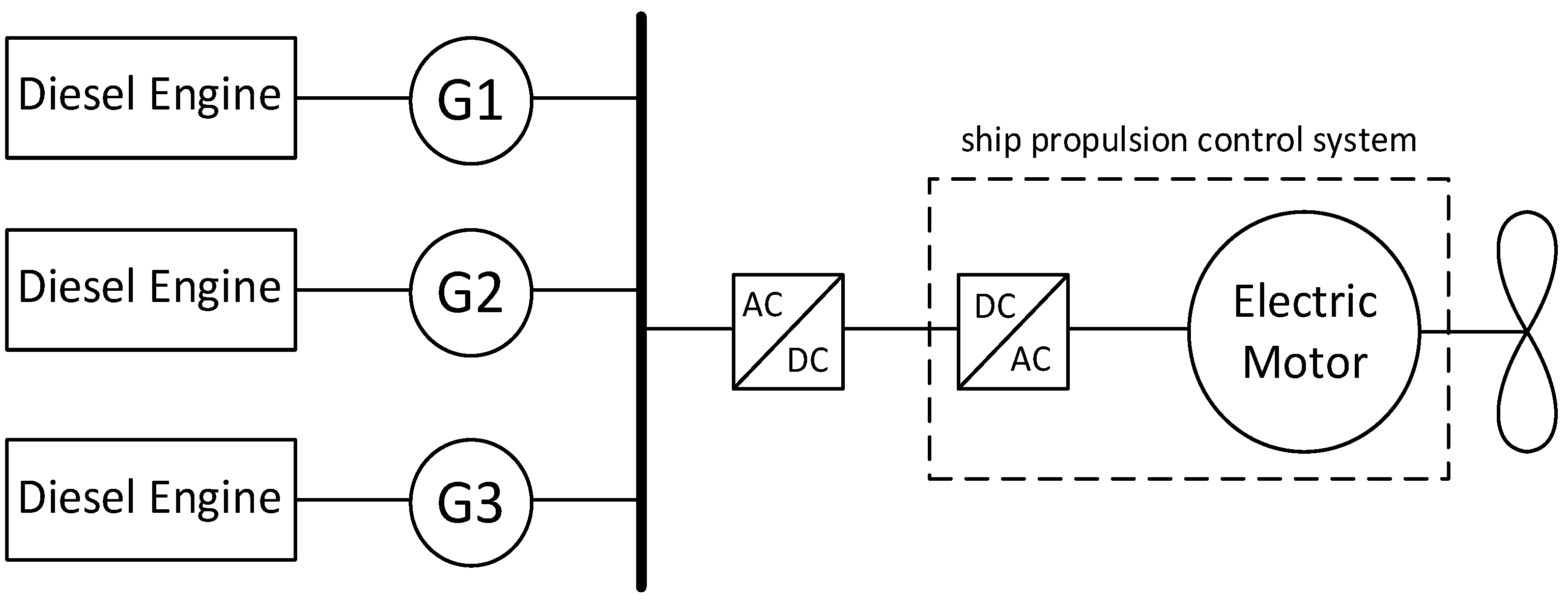
2.1. Energy Optimization of the PMSM Propulsion System in a Steady State Based on the Use of the Physical Properties of the System

This subsection will present an energy optimization method based on the analysis of steady-state electromagnetic processes, which was compared to the classic FOC control method. Analysis and simulation studies confirming the effectiveness of the method were carried out using the MATLAB Simulink program.

The equivalent electrical diagram of the PMSM propulsion system is presented in Figure 3.

The PMSM control system is based on the selection of a coordination system in such a way that variables defining its dynamics are constant in a steady state.

The UM mathematical description is conducted in the synchronously rotating system of d, q coordinates, which are closely connected with the PMSM magnetic field. The d axis coincides with the magnetic field vector. Then the electromagnetic force E will coincide with the q axis. The nonlinear model of the PMSM machine can be written in the form of a system of differential Equation (1).

$$\begin{array}{l}{U}_{acd}(t)=r_1{I}_d(t)+L_1\frac{d{I}_d(t)}{dt}-\omega L_1{I}_q(t),\\ U_{acq}(t)=r_1{I}_q(t)+L_1\frac{d{I}_q(t)}{dt}+\omega L_1{I}_d(t)+{\psi }_0\omega ,\\ T_e=1.5p{\psi }_0{I}_q(t),\\ J\frac{d{\omega }_m}{dt}=T_e-T_L.\end{array}$$

(1)

where:

U_acd(t), U_acq(t), I_d(t), I_q(t)—the inverter output voltage and stator currents (PMSM) on the d and q axes;

ω = pω_m—voltage pulsation at the inverter output;

ω_m—angular speed of the machine’s rotor;

J—inertia;

p—number of machine’s pole pairs;

T_e—electromagnetic moment of the machine;

T_L—load torque;

r₁—stator winding phase resistance;

x₁ = ωL₁ = p ω_mL₁—inductive reactance of the stator winding phase (L₁—inductance of the stator winding phase).

By analyzing the system (1), it is easy to notice that for specified ω_m and T_L there are an infinite number of equilibrium points (steady states) of the system, associated with input pairs (U_acd, U_acq).

Therefore, there is a natural problem of selecting a pair of inputs (controls) U_acd* and U_acq* in such a way as to ensure the reset of the system’s reactive power (Q_ac = 0), which we will refer to as energy optimization [21,29,30].

For this purpose, we conduct the following analysis:

In the steady state, electromagnetic processes presented by Equation (1), describing the propulsion, take the following form:

$$\begin{array}{l}{U}_{acd}=r_1{I}_d-x_1{I}_q,\\ U_{acq}=r_1{I}_q+x_1{I}_d+E_q.\end{array}$$

(2)

where:

$E_q=p{\omega }_m{\psi }_0=\omega {\psi }_0$—electromotive force of the PMSM stator.

The Equation (2) can be presented in a vector form as follows:

$${\overline{U}}_{ac}=\overline{E}+r_1{\overline{I}}_1+j{x}_1{\overline{I}}_1$$

(3)

where:

${\overline{U}}_{ac},{\overline{I}}_1,{\overline{\psi }}_0$, $\overline{E}=j\omega {\overline{\psi }}_0$—resultant (spatial) vector of variable electromagnetic states of the system.

In the mathematical description, the variables in Equation (3) are vector values. This enables building a vector diagram and evaluating the physical properties of the system. Figure 4 shows the vector diagram for the inverter–PMSM system with energy optimization.

By performing the energy optimization (Figure 4), U_acd, U_acq control signals in d, q coordinates are set in such a way that the phase shift between the voltage vector ${\overline{U}}_{ac}$ and the current vector ${\overline{I}}_1$ at the inverter output is equal to zero (φ = 0) (Figure 4). This is equivalent to resetting the reactive power Q_ac = 0.

In the optimal mode of operation, the modulation phase can be determined on the basis of the geometric relations of the vector diagram:

$${\phi }_{m.opt}=arcsin\frac{x_1{I}_1}{E}=arc\sin \frac{L_1{I}_1}{{\psi }_0}$$

(4)

In order to obtain energy optimization in the inverter–PMSM system, a pair of control inputs ought to be selected in accordance with the following equations:

$$\begin{array}{l}{U}_{acd}^{*}=-U_{ac}\sin {\phi }_{m.opt},\\ U_{acq}^{*}=U_{ac}\cos {\phi }_{m.opt}.\end{array}$$

(5)

Currents in longitudinal (d) and transverse (q) axes can be determined on the basis of the following relations:

$$\begin{array}{l}{I}_d=-I_1\sin {\phi }_{m.opt},\\ I_q=I_1\cos {\phi }_{m.opt}.\end{array}$$

(6)

from which it is easy to determine the current $I_1$ defining the angle ${\phi }_{m.opt}$ on the basis of Equation (4).

Now, having ${\phi }_{m.opt}$ and generating voltages $U_{ac}$ as an output from the PID controller (driven by the error $\Delta {\omega }_m={\omega }_m-{\omega }_m^{*}$), Equation (5) determines the desired pair of controls U_acd* and U_acq* ensuring energy optimization in a steady state.

Note that in the dynamic (transition) states, the adopted PID-type control is far from optimal, and it is even difficult to achieve any desired specifications here.

Formally, the inverter output voltage is determined from the geometric relations of the vector diagram:

$$U_{ac}=p{\omega }_m^{\ast }{\psi }_0\cos {\phi }_{m.opt}+r_1{I}_1^{\ast }$$

(7)

Due to the fact that energy characteristics of the PMSM propulsion can be determined from the following equations:

$$\begin{array}{l}{P}_{ac}=1.5(U_{acd}{I}_d+U_{acq}{I}_q),\\ Q_{ac}=1.5(U_{acq}{I}_d-U_{acd}{I}_q).\end{array}$$

(8)

it is easy to check (by simple substitution) that the initial assumption (phase shift between the voltage vector ${\overline{U}}_{ac}$ and the current vector ${\overline{I}}_1$ at the inverter output is equal to zero) leads to the reset of reactive power, i.e., $Q_{ac}=1.5(U_{acq}^{\ast }{I}_d^{}-U_{acd}^{\ast }{I}_q^{})=0$. The electromagnetic moment (T_e) in the steady state is equal to

$$T_e=\frac{2}{3}p{\psi }_0{I}_q$$

(9)

The calculations were based on the data of an exemplary PMSM used in the ship’s propulsion (

Table 1. Data of an exemplary PMSM used in the ship’s propulsion.

Parameter	Volume (Nominal Units)	Volume (Per Unit)
Rated Mechanical Power	2.0 MW	1
Rated Apparent Power	2.2419 MVA	1
Rated Line-to-Line Voltage	690 V (rms)	1
Rated Phase Voltage	398.4 V (rms)	1
Rated Stator Current	1867.76 A (rms)	1
Rated Stator Frequency	9.75 Hz	1
Rated Power Factor	0.8921	1
Rated Rotor Speed	22.5 rpm	1
Number of Pole Pairs	26	1
Rated Mechanical Torque	848.826 kNm	1
Rated Rotor Flux Linkage	5.8264 Wb (rms)	0.896
Stator Winding Resistance, R1	0.821 mΩ	0.00387
Moment of Inertia, J	6 kgm2	1
d-Axis Synchronous Inductance, Ld	1.5731 mH	0.4538
q-Axis Synchronous Inductance, Lq	1.5731 mH	0.4538

) [31].

Energy processes (dependencies: P_ac and Q_ac to ω_m and T_e) calculated with the use of Equations (4)–(8) are presented in Figure 5.

Analytical results of PMSM control with energy optimization shown in Figure 5 confirm the effectiveness of the proposed method. The reactive power Q_ac over the entire range of speed ω_m and electromagnetic torque T_e variation is zero (Figure 5b).

The electric propulsion system with PMSM, realizing energy optimization in the steady state (Q_ac = 0), is presented in Figure 6. The system includes the following:

• Voltage inverter composed of transistors (VT1–VT6) and diodes;
• Synchronous machine (PMSM);
• Rotor condition sensor (SPS);
• Coordinate transformation module (abc/d,q—Park–Gorev transformation);
• Coordinate transformation module (d,q/abc—Park–Gorev inverse transformation);
• Pulse width modulator (PWM);
• Speed controller (SC);
• Optimization block (OB).

In order to compare the control results of the PMSM system without and with energy optimization, the commonly used field-oriented control (FOC) method was implemented in MATLAB Simulink [32,33]. Figure 7 shows the energy processes in the inverter–PMSM drive system during speed and torque changes without energy optimization.

The test results of the commonly used PMSM control method (FOC), shown in Figure 7, prove that although the system responds correctly to the changes in the set speed ω*_m and torque T_e*, the presence of non-zero reactive power Q_ac in the inverter–PMSM system causes additional losses (losses in the inverter, in the connecting wires, and in the machine).

The preset load torque T_L (T_e*) and the preset angular velocity are assumed to be constant only during the design process. In fact, T_L is a disturbance, acting on the system, which can be realized in different ways (it may, e.g., depend on angular velocity). All changes in T_L (or ω*_m) can be interpreted as changes in the system equilibrium point. As the designed closed-loop system is stable, the system state just tracks the varying equilibrium point. Note that the step change of T_L (as in the paper) can be considered the strongest (worst) impact on the system.

The adopted PMSM propulsion system control strategy with energy optimization (Q_ac = 0) in the steady state was implemented in the MATLAB Simulink program on the basis of the model (Figure 6). PMSM parameters are shown in Table 1. During the tests, torque, rotational speed, stator currents in the d, q system, and active and reactive power during the operation of the propulsion system with energy optimization were compared. Figure 8 present the results of simulation tests. The waveforms indicate the behavior of electromagnetic torque (T_e) in relation to the set load torque T_L*, speed ω_m in relation to the set speed ω_m*, active power (P_ac), reactive power (Q_ac), and stator currents (on d and q axes) I_d and I_q in the inverter–PMSM system.

The test results of the proposed PMSM control method, shown in Figure 8, based on the analysis of steady-state electromagnetic processes, show the correct response of the system to changes in the set speed and torque (similar to the classical control method (Figure 7)) while reducing the reactive power to zero at the same time. Additional losses in the inverter–PMSM system associated with reactive power do not occur. Simulation studies confirmed the analytical research presented earlier. The proposed control method enabled energy optimization in a steady state to be obtained. In the dynamic state (t = 2 s), during the change (reduction tests) in speed, there are oscillations in the electromagnetic torque Te. This is connected with the fact that the synthesis of the speed controller in the classic system is conducted in accordance with the criteria of the so-called “technical optimum” [34].

2.2. Synthesis and Optimization of Dynamic and Static Control of a Propulsion System with PMSM

An alternative approach to the issue, having the advantage that we can additionally obtain optimal control in dynamic (transient) states, is the use of control theory methods [35,36,37,38,39].

In order to optimize the operation of the propulsion system in a dynamic state, taking into account energy optimization (Q_ac = 0), an analysis with the use of input–output (I/O) linearization and optimal control techniques was carried out.

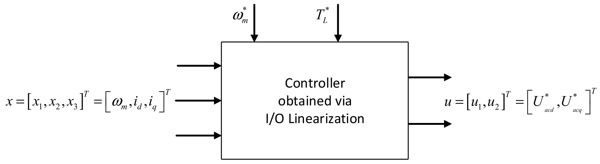
2.2.1. Design of the Main Controller via I/O Linearization Method

To facilitate the analysis and for the sake of clarity, the traditional notations in the control theory have been adopted. Let us first write Model (1) in the following state-space form:

$$\begin{array}{l}\frac{d{x}_1}{dt}=-\frac{r_1}{L_1}{x}_1+p{x}_3{x}_2+\frac{1}{L_1}{u}_1\\ \frac{d{x}_2}{dt}=-p{x}_3{x}_1-\frac{r_1}{L_1}{x}_2-\frac{p{\psi }_0}{L_1}{x}_3+\frac{1}{L_1}{u}_2\\ \frac{d{x}_3}{dt}=\frac{1.5p{\psi }_0}{J}{x}_2-\frac{1}{J}{T}_L\end{array}$$

(10)

where:

• x₁ = I_d, x₂ = I_q, x₃ = ω_m;
• u₁ = U_acd, u₂ = U_acq.

In addition, the model parameters are the same as in Table 1; i.e., r₁ = 0.821 mΩ, L₁ = 1.5731 mH, p = 26, Y₀ = 5.8264 Wb, J = 6 kgm², T_L = 848.826 kNm.

The considered control problem is to stabilize the state variable $x_3$ on the desired $x_3^{\ast }$ value, i.e., bring the system output

$$y=x_3-x_3^{*}$$

(11)

to zero, by using control variables u₁ and u₂, where $x_3^{*}={\omega }_m^{*}$ denotes the desired value of ω_m.

Analyzing the form of the above nonlinear system (10), one can observe that for controlling the output y it is enough to manipulate only the control variable u₂ while u₁ may serve us as an extra (constant) control parameter which will be then used for the system energetic optimization.

The synthesis of control u₂ can be performed by the input–output (I/O) feedback linearization, a method well known in the field of nonlinear control system engineering [27].

Based on this method, we transform Models (10) and (11) to the canonical form suitable for the direct derivation of the control law u₂.

However, to avoid the formalism of Lie derivatives, characteristic here, we repeatedly differentiate the output (11) with respect to time until the appearance of control u₂.

First we denote $y_1=y$.

Hence, using (10), we obtain the following:

$${\dot{y}}_1=\frac{1.5p{\psi }_0}{J}{x}_2-\frac{T_L}{J}\triangleq y_2$$

(12)

Differentiating (12) once more (and again using (10)), we obtain the following:

$${\dot{y}}_2=\frac{1.5p{\psi }_0}{J{L}_1}\left(-p{L}_1{x}_3{x}_1-r_1{x}_2-p{\psi }_0{x}_3+u_2\right)$$

(13)

Thus, we obtain the canonical form of some (sub)system of (10):

$$\begin{array}{l}{\dot{y}}_1=y_2\\ {\dot{y}}_2=f(x)+g(x)u_2\end{array}$$

(14)

where:

$$\begin{array}{l}{y}_1=y=x_3-x_3^{*},\\ y_2={\dot{y}}_1=\frac{1.5p{\psi }_0}{J}{x}_2-\frac{T_L}{J}.\end{array}$$

and

$$\begin{array}{l}f(\mathit{x})=\frac{1.5p{\psi }_0}{J{L}_1}\left(-p{L}_1{x}_3{x}_1-r_1{x}_2-p{\psi }_0{x}_3\right),\\ g(\mathit{x})=\frac{1.5p{\psi }_0}{J{L}_1}.\end{array}$$

(15)

As the control we are looking for has the following general form:

$$u_2=\frac{-f(x)+k_1{y}_1+k_2{y}_2}{g(x)}$$

(16)

we obtain the following specific formula:

$$u_2=(r_1{x}_2+p{\psi }_0{x}_3+p{L}_1{x}_3{x}_1)+\frac{J{L}_1}{1.5p{\psi }_0}(k_1{y}_1+k_2{y}_2)$$

(17)

which, to be implemented, requires measuring access to the whole system state components x₁, x₂, and x₃.

The resulting feedback system for the transformed system (10) is therefore of the following form:

$$\begin{array}{l}{\dot{y}}_1=y_2\\ {\dot{y}}_2=k_1{y}_1+k_2{y}_2\end{array}$$

Writing the last system in the matrix form

$$\left[\begin{array}{c}{\dot{y}}_1\\ {\dot{y}}_2\end{array}\right]=\left[\begin{array}{cc}0& 1\\ 0& 0\end{array}\right]\left[\begin{array}{c}{y}_1\\ y_2\end{array}\right]+\left[\begin{array}{c}0\\ 1\end{array}\right]u$$

(18)

where:

$$u=\left[\begin{array}{cc}{k}_1& k_2\end{array}\right]\left[\begin{array}{c}{y}_1\\ y_2\end{array}\right]=k_1{y}_1+k_2{y}_2$$

and selecting the standard quadratic optimality criterion

$$J(u)={\displaystyle {\int }_0^{\infty }(y^{T}Cy+uDu})dt\to \text{min}$$

where C and D are criterial matrices of proper dimensions, we can see that this controllable system can be appropriately (optimally) stabilized by the right selection of the gains k₁ and k₂ via, e.g., the LQR technique. In other words, the proper choice of these gains can ensure the required transient process of the system after a step change of certain quantities, e.g., the desired value of ω_m or the load torque T_L.

2.2.2. Analysis of the System Zero Dynamics

The partial transformation of the coordinates from x to y is defined by Equation (15). After this transformation, we have obtained a new system (14) of the second order, representing the external dynamics. As the original systems (10) and (11) are of the third order, the missing part of the dynamics should be completed with the internal (zero) dynamics (of the first order). The proof of the stability of the internal dynamics plays a key role in the successful application of the I/O linearization method, as it guarantees the stability of the whole (original) system (10).

To analyze the system zero dynamics, it is enough to examine the original systems (10) and (11) assuming that their outputs are identically equal to zero. This leads to the system’s restricted motion [27] being confined to the following set:

$$\begin{array}{l}{Z}^{\ast }=\left\{x:h(x)=L_{f}h(x)=0\right\}=\left\{x:x_3-x_3^{\ast }=0;\frac{1.5p{\psi }_0}{J}{x}_2-\frac{T_L}{J}=0\right\}\\ =\left\{x:x_3={\omega }_m;x_2=\frac{T_L}{1.5p{\psi }_0}\right\}\end{array}$$

(19)

where:

$$y=h(x)=x_3-x_3^{\ast }$$

The motion of the original systems (10) and (11) on $Z^{\ast }$, with the input [35]

$$u_2^{*}={\frac{-f(x)}{g(x)}}_{\left|x\in Z^{\ast }\right.}=-p{L}_1{x}_3{x}_1-r_1{x}_2-p{\psi }_0{x}_3$$

represents the system zero dynamics:

$$\frac{d{x}_1}{dt}=-\frac{r_1}{L_1}{x}_1+p{x}_3{x}_2+\frac{1}{L_1}{u}_1$$

(20)

As the term $p{x}_3{x}_2$ is constant (see (19)) and $u_1$ is also taken as a constant parameter, this dynamics takes the form of a stable linear system:

$$\frac{d{x}_1}{dt}=-\frac{r_1}{L_1}{x}_1+const$$

(21)

By choosing $u_1$ so that $-p{x}_3{x}_2=\frac{1}{L_1}{u}_1$, we can make the above system also asymptotically stable.

In this way, we have proved that the control (16) found above stabilizes the whole nonlinear system (10) regardless of the choice of the control u₁ (in the form of some constant parameter; compare (22)).

2.2.3. Energetic Optimization of the System Operation in Steady State

By choosing the control parameter $u_1$ appropriately, we may achieve some extra properties of the system (10) in the steady state. We can, e.g., perform an energetic optimization of the system operation by guaranteeing that the system reactive power is equal to zero.

Observe that by applying saturating control of the following form:

$$u_1=a\cdot sat\left(\frac{-p{L}_1{x}_3{x}_2}{a}\right)$$

(22)

where:

• a > 0—control parameter
• we have a chance (by an appropriate choice of the parameter a) to influence the value of variable x₁ (in the steady state) without affecting the evolution (transient process) of the variables x₁ and x₂.

This way, we have the possibility to perform some steady-state system optimization.

At this point, it seems reasonable to perform an energetic optimization of the system operation in the steady state, i.e., to guarantee that the system reactive power (cf. (8)) equals zero:

$$Q_{ac}=1.5(U_q{I}_d-U_d{I}_q)=1.5(u_2{x}_1-u_1{x}_2)=0$$

(23)

To analyze the system (11) in the steady state, we assume that the derivatives on the left-hand side are equal to zero.

Having access to the system state components x₁, x₂, and x₃, we can see (from the first equation of (10)) that $u_1=r_1{x}_1-p{L}_1{x}_2{x}_3$.

Since, in the steady state, u₁ = a (cf. (22)), we have the following:

$$x_1(a)=(p{L}_1{x}_2{x}_3+a)/r_1$$

(24)

Now, from the second equation of (11), we obtain the following:

$$u_2(a)=p{L}_1{x}_1(a)x_3+r_1{x}_2+p{\psi }_0{x}_3$$

(25)

In summary, the reactive power in the steady state is as follows:

$$Q_{ac}(a)=1.5(u_2{x}_1-u_1{x}_2)=1.5(u_2(a)x_1(a)-a{x}_2)$$

(26)

To obtain Q_ac(a) = 0, we have to just solve simple quadratic Equation (26) with respect to parameter a.

On the other hand, we can also influence the quality of the system transient process (e.g., during a load T_L step change) by appropriate selection of the gains k₁ and k₂ (cf. (18)). It should be noted that for the implementation of the controller (17) and (22), the value of the load T_L need not be known.

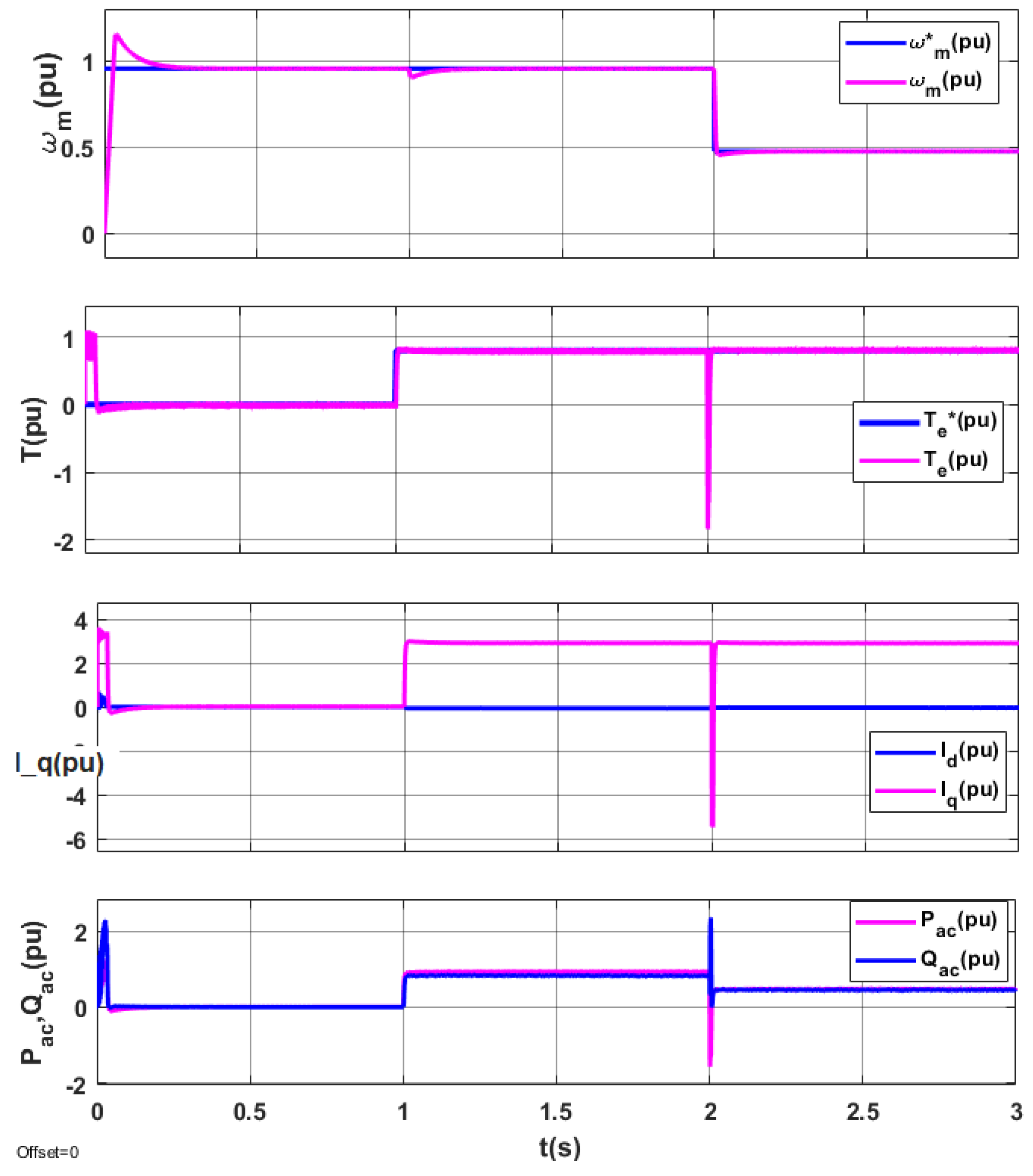
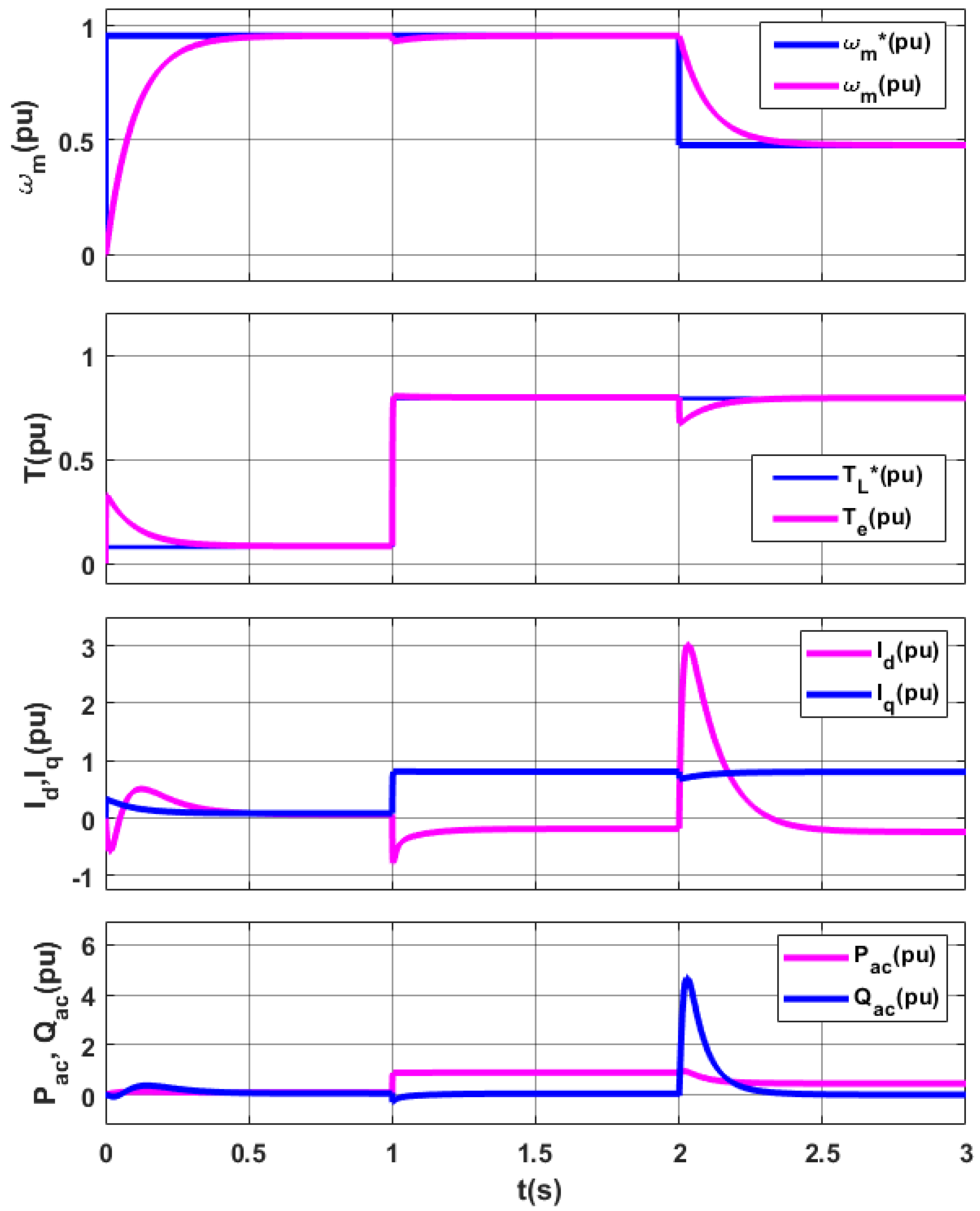
2.2.4. Tests of the Propulsion System with PMSM Using Synthesized Control

Based on the above-mentioned analysis, tests with the use of the MATLAB Simulink program for the DE propulsion control system of the ship (with synthesized control) were carried out. A block diagram of the linearized I/O system with energy optimization (Q_ac) is presented in Figure 9.

Control signals U_acd and U_acq, worked out by the controller system in accordance with the strategy presented above, are setpoints for the Park–Gorev inverse transformation in the PMSM control system (Figure 6).

Simulation tests of the PMSM propulsion system with the use of the I/O linearization method allowing for dynamic optimization and energy optimization (Q_ac) in steady state were conducted on the basis of the model implemented in the MATLAB Simulink program. Figure 10 presents the behavior of the electromagnetic torque (T_e) in relation to the set load torque T_L*, speed ω_m in relation to the set speed ω_m*, active power (P_ac) and reactive power (Q_ac), and stator currents I_d and I_q (d and q axes) in the inverter–PMSM system.

The test results of the proposed PMSM control method shown in Figure 10 show energy optimization (Q_ac = 0) of the inverter–PMSM system in the steady state similarly to the first proposed method (Figure 8). At the same time, the correct response of the system in dynamic states should be noted. There is no oscillation of the moment when the speed is changed, as was the case with the first method.

3. Discussion

The article presents two methods of controlling the ship’s electric propulsion. They enable obtaining energy optimization of the system by reducing the reactive power in the inverter–PMSM system (Q_ac = 0).

The results of analytical tests (Figure 5) confirmed in the simulation tests (Figure 8) of the modified classic method regarding the PMSM control, based on the analysis in the steady state, enabled optimizing the mechatronic propulsion system of the ship in terms of the energy criterion. Reactive power in the inverter–PMSM system has been (practically) reduced to zero. Therefore, the currents and losses in transmission lines (in the inverter and in PMSM) were limited.

The simulation results of the modified classic method of PMSM propulsion control (Figure 8) indicate the appropriate reaction of the system to the change of the set parameters (T_L*, ω_m*) in the steady state. This results from the assumptions of the method. Oscillations in the electromagnetic torque T_e (t = 2 s), when changing the set speed, are connected with the lack of proper control of the system operation in the dynamic (transient) mode.

To cope with this problem, this article also proposes an alternative approach based on the methods of control theory (Section 2.2). The I/O linearization technique associated with the LQR method, from the area of optimal control, was used for a nonlinear PMSM model with energy optimization (Q_ac = 0).

The results of simulation tests for this control method, presented in Figure 10, demonstrate the same reaction of the system in the steady state as in the classic method (Figure 8). In the steady state, the reactive power Q_ac in the inverter–PMSM system is equal to zero (energy optimization). Note however that in the dynamic mode (at the change of a set speed, t = 2 s), there are no oscillations in the electromagnetic torque (T_e), as was observed in the classic control method (which copes only in the steady state).

The paper does not address the problem of knowledge of the model parameters and their errors. However, the influence of disturbances in the form of variable (step change) T_L (or ω*_m) has been considered. It should be noted that the approach presented in Section 2.2 allows for straightforward generalization to the adaptive version (cf. [40]) which is in preparation.

4. Conclusions

Methods of reactive power compensation based on instantaneous power analysis [41,42] in electrical systems and reactive power reduction in drive systems with PMSMs based on steady-state analysis (e.g., [43,44,45,46]) are known. Most of these methods are characterized by a complex control algorithm or a complicated system topology.

The first method proposed in the article (Section 2.1), whose simple control algorithm is based on steady-state analysis, is an effective energy optimization without significantly burdening the processor unit in the control system. The disadvantage of this method, as demonstrated by tests, is torque oscillations when dynamic changes in torque or speed occur.

The ship propulsion PMSM control strategy proposed in Section 2.2 (the second method), based on the I/O linearization technique associated with the LQR method, is effective for steady-state energy optimization. In addition, it eliminates the disadvantage of the first method by optimizing the system in transients, as studies have shown. The authors recommend this control method in ship propulsion systems where rapid changes in propulsion load occur (especially in bad weather conditions). The authors have not found a control method in the literature that integrates these two functions (steady-state energy optimization and transient optimization).

The optimal control system synthesis of the PMSM electric drive can also be used in other PMSM drives, especially in high-power drives, where it is important to reduce reactive power in the inverter–PMSM system. For drives used on land, where there are no dynamic changes in load and speed (e.g., fans in industry), the first method is recommended because the control algorithm is simple (no load on the processor unit).

References

1. UNCTAD. Review of Maritime Transport 2018; United Nations Publication: New York, NY, USA, 2018; pp. 23–26. Available online: https://unctad.org/system/files/official-document/rmt2018_en.pdf (accessed on 5 May 2022).
2. IMO RESOLUTION MEPC.203(62) Adopted on 15 July 2011. Available online: https://wwwcdn.imo.org/localresources/en/KnowledgeCentre/IndexofIMOResolutions/MEPCDocuments/MEPC.203(62).pdf (accessed on 5 May 2022).
3. Polakis, M.; Zachariadis, P.; Kat, J.O. The Energy Efficiency Design Index (EEDI). In Sustainable Shipping; Springer: New York, NY, USA, 2019; pp. 93–135. [Google Scholar] [CrossRef]
4. International Maritime Organization. IMO Train the Trainer (TTT) Course on Energy Efficiency Ship Operation. In Module 2—Ship Energy Efficiency Regulations and Related Guidelines; International Maritime Organization: London, UK, 2016; Available online: https://wwwcdn.imo.org/localresources/en/OurWork/Environment/Documents/Air%20pollution/TTT%20trainers%20manual%20final2.pdf (accessed on 5 May 2022).
5. Grljušić, M.; Medica, V.; Radica, G. Calculation of Efficiencies of a Ship Power Plant Operating with Waste Heat Recovery through Combined Heat and Power Production. Energies 2015, 8, 4273–4299. [Google Scholar] [CrossRef] [Green Version]
6. Mrzljak, V.; Zarkovic, B.; Prpic-Orsic, J. Marine slow speed two-stroke diesel engine—Numerical analysis of efficiencies and im-portant operating parameters. Mach. Technol. Mater. 2017, 11, 481–484. [Google Scholar]
7. Zaccone, R.; Campora, U.; Martelli, M. Optimization of a diesel-electric ship propulsion and power generation system using a genetic algorithm. J. Mar. Sci. Eng. 2021, 9, 587. [Google Scholar] [CrossRef]
8. Hansen, J.F.; Wendt, F. History and State of the Art in Commercial Electric Ship Propulsion, Integrated Power Systems, and Future Trends. Proc. IEEE 2015, 103, 2229–2242. [Google Scholar] [CrossRef]
9. Vossen, C. Diesel electric propulsion on ∑IGMA class corvettes. In Proceedings of the 2011 IEEE Electric Ship Technologies Symposium, Alexandria, VA, USA, 10–13 April 2011; pp. 288–291. [Google Scholar] [CrossRef]
10. Acanfora, M.; Balsamo, F.; Fantauzzi, M.; Lauria, D.; Proto, D. Load levelling through Storage System for Hybrid Diesel Electric Ship Propulsion in Irregular Wave Conditions. In Proceedings of the 2022 International Symposium on Power Electronics, Electrical Drives, Automation and Motion (SPEEDAM), Sorrento, Italy, 22–24 June 2022; pp. 640–644. [Google Scholar] [CrossRef]
11. Fan, Z.; Liang, C.; Dong, Y.; Chang, G.; Pan, W.; Shao, S. Control of the Diesel-Electric Hybrid Propulsion in a Practical Cruise Vessel. In Proceedings of the 2021 IEEE International Conference on Power, Intelligent Computing and Systems (ICPICS), Shenyang, China, 29–31 July 2021; pp. 311–316. [Google Scholar] [CrossRef]
12. Veksler, A.; Johansen, T.J.; Skjetne, R.; Mathiesen, E. Thrust Allocation With Dynamic Power Consumption Modulation for Diesel-Electric Ships. IEEE Trans. Control Syst. Technol. 2016, 24, 578–593. [Google Scholar] [CrossRef] [Green Version]
13. Zhu, H.H.; Dong, Z. Modeling and Simulation of Hybrid Electric Ships with AC Power Bus—A Case Study. In Proceedings of the 2018 14th IEEE/ASME International Conference on Mechatronic and Embedded Systems and Applications (MESA), Oulu, Finland, 2–4 July 2018; pp. 1–8. [Google Scholar] [CrossRef]
14. WARTSILA. Improving Efficiency. Available online: https://www.wartsila.com/sustainability/innovating-for-sustainability/improving-efficiency (accessed on 5 May 2022).
15. Kozak, M. Alternating Current Electric Generator Machine Inverters in a Parallel Power Sharing Connection. IEEE Access 2019, 7, 32154–32165. [Google Scholar] [CrossRef]
16. Kozak, M. New concept of ship’s power plant system with varying rotational speed gensets. In Proceedings of the 58th international conference of machine design departments (ICMD 2017), Prague, Czech Republic, 6–8 September 2017; pp. 170–175. [Google Scholar]
17. Choi, I.C.; Jeung, Y.-C.; Lee, D.-C. Variable speed control of diesel engine-generator using sliding mode control. In Proceedings of the 2017 IEEE Transportation Electrification Conference and Expo, Asia-Pacific (ITEC Asia-Pacific), Harbin, China, 7–10 August 2017; pp. 1–5. [Google Scholar] [CrossRef]
18. Rezkallah, M.; Dubuisson, F.; Singh, S.; Singh, B.; Chandra, A.; Ibrahim, H.; Ghandour, M. Coordinated Control Strategy for Hybrid off-Grid System Based on Variable Speed Diesel Generator. IEEE Trans. Ind. Appl. 2022, 58, 4411–4423. [Google Scholar] [CrossRef]
19. Hu, Y.; Cirstea, M.; McCormick, M.; Haydock, L. Modelling and simulation of a variable speed stand-alone generator system. In Proceedings of the 2000 Eighth International Conference on Power Electronics and Variable Speed Drives (IEE Conf. Publ. No. 475), London, UK, 18–19 September 2000; pp. 372–377. [Google Scholar] [CrossRef]
20. Zhou, Z.; Camara, M.B.; Dakyo, B. Coordinated Power Control of Variable-Speed Diesel Generators and Lithium-Battery on a Hybrid Electric Boat. IEEE Trans. Veh. Technol. 2017, 66, 5775–5784. [Google Scholar] [CrossRef]
21. German-Galkin, S.; Tarnapowicz, D. Energy Optimization of Ship’s Shaft Generator with Permanent Magnet Synchronous Generator. Nase More 2020, 67, 138–145. [Google Scholar] [CrossRef]
22. Jamieson, P. Innovation in Wind Turbine Design, 2nd ed.; John Wiley & Sons, Ltd.: Hoboken, NJ, USA, 2018; ISBN 978-1-119-13790-0. [Google Scholar]
23. Ludwig, F.; Möckel, A. Operation method for AC grid powered PMSM with open-end winding in dual-inverter topology for power factor maximization. In Proceedings of the 8th IET International Conference on Power Electronics, Machines and Drives (PEMD 2016), Glasgow, UK, 19–21 April 2016; pp. 1–5. [Google Scholar] [CrossRef]
24. Jianbo, C.; Yuwen, H.; Wenxin, H.; Yong, L.; Jianfei, Y.; Mingjin, W. Direct active and reactive power control of PMSM. In Proceedings of the 2009 IEEE 6th International Power Electronics and Motion Control Conference, Wuhan, China, 17–20 May 2009; pp. 1808–1812. [Google Scholar] [CrossRef]
25. Lei, J.; Zhou, B.; Bian, J.; Qin Jiangsu, X. Unit power factor control of PMSM fed by indirect matrix converter. In Proceedings of the 2014 17th International Conference on Electrical Machines and Systems (ICEMS), Hangzhou, China, 22–25 October 2014; pp. 926–930. [Google Scholar] [CrossRef]
26. Cimini, G.; Ippoliti, G.; Orlando, G.; Pirro, M. PMSM control with power factor correction: Rapid prototyping scenario. In Proceedings of the 4th International Conference on Power Engineering, Energy and Electrical Drives, Istanbul, Turkey, 13–17 May 2013; pp. 688–693. [Google Scholar] [CrossRef]
27. Khalil, H.K. Nonlinear Systems, 3rd ed.; Prentice Hall: Upper Saddle River, NJ, USA, 2002; pp. 509–521. ISBN 978-0130673893. [Google Scholar]
28. Lewis, F.L.; Draguna Vrabie, D.; Syrmos, V.L. Optimal Control, 3rd ed.; John Wiley & Sons, Inc.: Hoboken, NJ, USA, 2012; ISBN 978-0470633496. [Google Scholar]
29. German-Galkin, S.; Tarnapowicz, D. Energy Optimization of the ‘Shore to Ship’ System-A Universal Power System for Ships at Berth in a Port. Sensors 2020, 20, 3815. [Google Scholar] [CrossRef] [PubMed]
30. German-Galkin, S.; Tarnapowicz, D. Optimization of the electric car’s drive system with PMSM. In Proceedings of the 12th International Science-Technical Conference AUTOMOTIVE SAFETY, Kielce, Poland, 21–23 October 2020. [Google Scholar] [CrossRef]
31. Wu, B.; Lang, Y.; Zargari, N.; Kouro, S. Appendix B: Generator Parameters. In Power Conversion and Control of Wind Energy Systems; IEEE: Manhattan, NY, USA, 2011; pp. 319–326. [Google Scholar] [CrossRef]
32. Zawirski, K. Permanent Magnet Synchronous Motor Control; Poznan University of Technology Publishing House: Poznań, Poland, 2005; ISBN 83-7143-337-9. [Google Scholar]
33. Kaczmarek, T.; Zawirski, K. Drive Systems with Synchronous Motor; Poznan University of Technology Publishing House: Poznań, Poland, 2000; ISBN 978-83-7348-401-6. [Google Scholar]
34. Kazmierkowski, M.P.; Tunia, H. Automatic Control of Converter-Fed Drives. In Studies in Electrical and Electronic Engineering, 1st ed.; PWN-Elsevier Science Publishers: Warsaw, Polland; Amsterdam, The Netherlands; New York, NY, USA; Tokyo, Japan, 1994; ISBN 13-978-0444986603. (In English) [Google Scholar]
35. Aghili, F. Optimal Feedback Linearization Control of Interior PM Synchronous Motors Subject to Time-Varying Operation Conditions Minimizing Power Loss. IEEE Trans. Ind. Electron. 2018, 65, 5414–5421. [Google Scholar] [CrossRef]
36. Fraga, R.; Sheng, L. Non linear and intelligent controllers for the ship rudder control. In Proceedings of the 2011 Saudi International Electronics, Communications and Photonics Conference (SIECPC), Riyadh, Saudi Arabia, 24–26 April 2011; pp. 1–5. [Google Scholar] [CrossRef]
37. Parvathy, A.K.; Devanathan, R.; Kamaraj, V. Application of quadratic linearization to control of Permanent Magnet synchronous motor. In Proceedings of the 2011 1st International Conference on Electrical Energy Systems, Chennai, India, 3–5 January 2011; pp. 158–163. [Google Scholar] [CrossRef]
38. Do, T.D.; Kwak, S.; Choi, H.H.; Jung, J.-W. Suboptimal Control Scheme Design for Interior Permanent-Magnet Synchronous Motors: An SDRE-Based Approach. IEEE Trans. Power Electron. 2014, 29, 3020–3031. [Google Scholar] [CrossRef]
39. Cheema, M.A.M.; Fletcher, J.E.; Xiao, D.; Rahman, M.F. A Linear Quadratic Regulator-Based Optimal Direct Thrust Force Control of Linear Permanent-Magnet Synchronous Motor. IEEE Trans. Ind. Electron. 2016, 63, 2722–2733. [Google Scholar] [CrossRef]
40. Zwierzewicz, Z. Robust and Adaptive Path-Following Control of an Underactuated Ship. IEEE Access 2020, 8, 120198–120207. [Google Scholar] [CrossRef]
41. Wang, F.; Mi, Z.; Yang, Q. Comparison between Periodic Function space based power theory and traditional power theory. In Proceedings of the 2008 International Conference on Electrical Machines and Systems, Wuhan, China, 17–20 October 2008; pp. 2212–2216. [Google Scholar]
42. Akagi, H.; Hirokazu-Watanabe, E.; Aredes, M. The Instantaneous Power Theory. In Instantaneous Power Theory and Applications to Power Conditioning; IEEE: Manhattan, NY, USA, 2017; pp. 37–109. [Google Scholar] [CrossRef]
43. Ho, T.-Y.; Chen, M.-S.; Chen, L.-Y.; Yang, L.-H. The design of a PMSM motor drive with active power factor correction. In Proceedings of the 2011 2nd International Conference on Artificial Intelligence, Management Science and Electronic Commerce (AIMSEC), Dengfeng, China, 8–10 August 2011; pp. 4447–4450. [Google Scholar] [CrossRef]
44. Tau, J.-H.; Tzou, Y.-Y. PFC control of electrolytic capacitor-less PMSM drives for home appliances. In Proceedings of the 2017 IEEE 26th International Symposium on Industrial Electronics (ISIE), Edinburgh, UK, 19–21 June 2017; pp. 335–341. [Google Scholar] [CrossRef]
45. Gokulapriya, R.; Pradeep, J. Shunt based active power factor correction circuit for direct torque controlled PMSM drive. In Proceedings of the 2017 Third International Conference on Science Technology Engineering & Management (ICONSTEM), Chennai, India, 23–24 March 2017; pp. 517–521. [Google Scholar] [CrossRef]
46. Vimal, M.; Sojan, V. Vector controlled PMSM drive with power factor correction using zeta converter. In Proceedings of the 2017 International Conference on Energy, Communication, Data Analytics and Soft Computing (ICECDS), Chennai, India, 1–2 August 2017; pp. 289–295. [Google Scholar] [CrossRef]
Figure 1. Traditionally used ship propulsion system in the diesel–electric system (AC grid).
Energies 15 09390 g001
Figure 2. Ship propulsion system in the diesel–electric system with optimization of the operation of generator propulsion engines (DC grid).
Energies 15 09390 g002
Figure 3. Equivalent diagram of the propulsion system with PMSM.
Energies 15 09390 g003
Figure 4. Vector diagram of inverter–PMSM system during energy optimization.
Energies 15 09390 g004
Figure 5. Energy characteristics: (a) active power Pac and (b) reactive power Qac with optimization.
Energies 15 09390 g005
Figure 6. PMSM control system with PWM and speed regulator with energy optimization (Qac = 0).
Energies 15 09390 g006
Figure 7. Energy processes (Pac, Qac) in inverter-PMSM drive system during speed and torque changes without energy optimization (FOC method).
Energies 15 09390 g007
Figure 8. Energy processes (Pac, Qac) in the inverter-PMSM propulsion system during changes in speed and torque with energy optimization.
Energies 15 09390 g008
Figure 9. Block diagram of I/O linearized system with energy optimization (Qac).
Energies 15 09390 g009
Figure 10. Energy processes (Pac, Qac) in the inverter-PMSM propulsion system during changes in speed and torque with energy optimization using the I/O linearization method.
Energies 15 09390 g010