Deep Learning with Dipper Throated Optimization Algorithm for Energy Consumption Forecasting in Smart Households

Abstract

One of the relevant factors in smart energy management is the ability to predict the consumption of energy in smart households and use the resulting data for planning and operating energy generation. For the utility to save money on energy generation, it must be able to forecast electrical demands and schedule generation resources to meet the demand. In this paper, we propose an optimized deep network model for predicting future consumption of energy in smart households based on the Dipper Throated Optimization (DTO) algorithm and Long Short-Term Memory (LSTM). The proposed deep network consists of three parts, the first part contains a single layer of bidirectional LSTM, the second part contains a set of stacked unidirectional LSTM, and the third part contains a single layer of fully connected neurons. The design of the proposed deep network targets represents the temporal dependencies of energy consumption for boosting prediction accuracy. The parameters of the proposed deep network are optimized using the DTO algorithm. The proposed model is validated using the publicly available UCI household energy dataset. In comparison to the other competing machine learning models, such as Random Forest (RF), Support Vector Machine (SVM), K-Nearest Neighbor (KNN), Multi-Layer Perceptron (MLP), Sequence-to-Sequence (Seq2Seq), and standard LSTM, the performance of the proposed model shows promising effectiveness and superiority when evaluated using eight evaluation criteria including Root Mean Square Error (RMSE) and $R^2$. Experimental results show that the proposed optimized deep model achieved an RMSE of (0.0047) and $R^2$ of (0.998), which outperform those values achieved by the other models. In addition, a sensitivity analysis is performed to study the stability and significance of the proposed approach. The recorded results confirm the effectiveness, superiority, and stability of the proposed approach in predicting the future consumption of energy in smart households.

1. Introduction

Building energy use is a major factor in the need for energy efficiency projects in many countries [1,2]. Inefficient regulation of thermal comfort, improper electrical equipment sequencing and start-up time, and overuse of appliances consuming energy, such as air conditioning systems, ventilation, heating, and exhaust fans, all contribute significantly to the waste of energy within buildings. To this end, the development of smart households equipped with a variety of control methods, measuring devices, and sensors [3] is crucial for the efficient management of building energy use. Predicting the energy consumption of individual homes is a crucial part of the management process required to actualize the response of the demand side. To better manage the operation and maintenance of electrical systems, utilities need accurate and precise forecasting of energy load in the short term at the household level. This would allow utilities to better plan and schedule their energy resources to coordinate power generation with load demand.

At the building level, the energy consumption profile [4] is made up of the following elements. There are three types of energy usage patterns: (1) variable consumption due to changes to the weather that may occur daily; (2) noise, which is hard to be physically represented; and (3) predictable consumption based on the building’s historical load patterns. Energy usage at the residential level is very variable and erratic because of the varying nature of the weather. Customers’ spending patterns may also shift due to other causes, such as the weather. Therefore, consumption is very unpredictable because it is based on the choices of individual consumers. Predicting the unpredictable patterns while also considering the stochastic nature of the behavior of customer consumption and the weather changes, is difficult in forecasting household-level energy consumption in the short term. For this reason, it is simpler to make very accurate predictions when looking at aggregated short-term load forecasts, as the overwhelming component corresponds to standard consumption patterns.

Since building energy usage is notoriously difficult to anticipate, cutting-edge deep learning algorithms have emerged as the method of choice for creating reliable forecasting tools. Recently, Much work has gone into developing strategies for aggregative load forecasting [5,6,7]. In [5], the historical yearly energy consumption estimates are used to distinguish aggregate sub-zones into clusters. Households were grouped, aggregate estimates were calculated for each cluster independently, and then the projections were aggregated in [6] to account for differences in household consumption patterns. In [7], a method for residential load aggregation was developed, and it was established what fraction of a cluster’s customers would benefit most from having smart meters with sub metering capacity installed. Nonetheless, there has been little progress in energy forecasting for the short term at the level of individual households. Time series analysis, ensemble and deep learning models, machine learning approaches, binary backtracking search algorithms, and metaheuristic optimization algorithms are all practical tools for forecasting and managing energy consumption in smart households [8,9,10,11,12]. Convolutional Neural Networks (CNNs) and Recurrent Neural Networks (RNNs) are two common models in the deep learning field that are usually employed for forecasting energy consumption. CNN is denoted by a neural network with feed-forward connections, whereas the time series RNN is denoted by cells in which the changing behavior of the feature across time is illustrated by its internal states. The RNN type known as Long Short Term Memory (LSTM) uses three gates to determine which inputs should be used in further processing and which should be discarded. Researchers have discovered that RNN models are less precise than LSTM models [13,14,15,16]. To achieve exact performance without a feature extraction step, CNNs have been used in early iterations of hybrid models [17,18]. However, the convolution procedure, the number of kernels, and the amount of memory used all have a role in the overall difficulty of CNN models. LSTM networks, on the other hand, are spatial and temporal, and their resource needs do not increase exponentially as the input size grows. As a result of these considerations, we employ a bidirectional LSTM layer to extract information from features rather than a sophisticated CNN layer, and we estimate energy usage by stacking LSTM layers atop dense layers. The proposed model is compared to another ensemble model and other popular hybrid models based on LSTM, ConvLSTM, and CNN-LSTM, to assess the overall performance.

A smart household consumes energy actively and is fitted with a sophisticated home energy management system [10]. Energy companies and homeowners alike can keep tabs on energy use with the help of smart meters that update in real-time. Using an ideal consumption plan, users may lower their energy bill with the help of a smart metering system and Home Energy Management Systems (HEMS) [9]. The HEMS can plan the consumption of household-controlled loads and storage units to achieve maximum efficiency. In addition, it may calculate the amount of excess energy generated by customers’ Distributed Generation (DG) units that can be sold back to the grid. The architecture of a typical household is depicted in Figure 1.

Nature frequently serves as an inspiration for metaheuristic optimization techniques. Different types of metaheuristic algorithms can be identified based on their respective inspirations. Primarily, we may classify algorithms that take cues from biological processes, such as evolution or animal social behavior. Many of the metaheuristics ideas come from scientific research. Physicists and chemists often provide inspiration for these algorithms. Additionally, artistically-motivated algorithms have proven effective in global optimization. They get inspiration for their own artistic endeavors mainly from the ways in which artists act (such as architects and musicians). Another type of algorithm that draws its motivation from social phenomena is one whose solutions to optimization problems are based on a simulation of collective behavior.

It is essential to consider the potential effects of the so-called “No free lunch theorems” while working with optimization problems. According to one of the theories, some optimization functions may be better served by Algorithm A than by Algorithm B. Algorithms A and B will, on average, yield the same result throughout the whole function space. Thus, there are no unquestionably superior algorithms. On the other hand, one may argue that averaging across all feasible functions is unnecessary for a particular optimization issue. The primary goal here is to identify optimal solutions that have nothing to do with arithmetically averaging across the range of feasible functions. While some scientists insist on a single, all-encompassing method, others argue that different optimization problems call for different approaches and that specific algorithms are more effective than others. Therefore, the primary goal would be to select the optimal algorithm for a particular problem or improve algorithms for most situations.

Among this work’s most significant contributions are understanding the correlations, complex patterns, and the high non-linearity in data that are inaccessible to traditional unidirectional architectures, a unique model based on hybrid deep learning is developed by stacking bidirectional and unidirectional LSTM models. A real-world case study shows how well the proposed model can predict appliance energy consumption in smart households. The performance of the proposed model is shown in contrast to the other recent methodologies via quantitative evaluations performed via score metrics. The impact of including lag energy aspects is analyzed, along with the architecture of the proposed model, the implications of the hyperparameters of the developed model, and the overall perception of doing so. Additionally, competing deep learning models are compared to the proposed model across the dataset to prove its superiority.

What follows is the outline for the rest of the paper. The literature overview on the machine learning applications and bidirectional LSTM models in residential energy forecasting are discussed in Section 2. The methods and materials utilized in this work are explained in Section 3. The details of the proposed optimized deep learning approach come in Section 4. Section 5 compares the results achieved by the proposed technique to those obtained by the baseline models. Section 6 concludes the findings of this work and presents the potential perspectives for future work.

2. Literature Review

Scientific interest in short-term load forecasting at the residential level has increased significantly due to the introduction of renewable energy sources to smart households [19]. It is crucial to properly assess the unexpected patterns of load demand at the consumer level to effectively balance loads and make optimal use of renewable energy sources. Initially, efforts to forecast short-term residential loads relied on standard statistical approaches and time series research. As curiosity in Artificial Intelligence (AI) has increased, several machines and deep learning methodologies have been introduced to forecasting households’ energy usage. Support Vector Regression (SVR) models and Multilayer Perceptron (MLP) trained with data on the structural features and elements of households are recommended by the authors of [20] for predicting cooling and heating loads in dwellings. A correlation of 0.99 was discovered between their proposed models and the data. The authors of [16] presented a two-stage forecasting technique. Initial procedures involved making load forecasts for the following day using standard time forecasting techniques. In the second step, they used quadratic models, linear regression, and Support Vector Machines (SVMs) to predict outliers, increasing our forecasts’ precision. When the estimates from the second stage were added to these outliers, the MAPE of the resulting projected values was 5.21%. A significant drawback of the SVM model is that its training time scales linearly with the number of data records, making it inappropriate for large datasets.

In [21], the authors proposed several methods for improving training data analysis, including generalized Extreme Learning Machines (ELMs) and improved wavelet neural networks. In these methods, predicted loads were presented as intervals due to the uncertainties inherent in the forecasting algorithms and the underlying data. ELMs are just neural networks with one hidden layer. Since ELMs’ generalization is poor and their reliance on prediction accuracy is improved, their activation function is generally ineffective. Wavelets, utilized as activation functions in their method, helped overcome these limitations. However, ELM-based techniques are limited in their ability to deeply extract the underlying information and features associated with data on energy use because they rely on a single layer of modeling.

Models of Elman and backpropagation neural networks were developed mathematically in [22]. The models were employed to handle the energy consumption time-varying aspects, and they learned at slow rates and store internal states through the model layers. Based on their findings, Elman neural networks are superior to backpropagation neural networks for predicting future dynamic loads. These neural network-based models, however, will invariably gravitate to suboptimal solutions. Consequences include vague generalization and overfitting.

Deep learning models have recently been the topic of extensive study because of their potential to rapidly and accurately identify patterns in data relating to energy consumption and make predictions about future usage. In most cases, deep learning models experience either bursting gradients or disappearing gradients. LSTM networks, which implement memory cells and computation gates, solve this issue. LSTMs have been used for load forecasting and time series analysis. Recent research in [23,24] employed extreme learning machines, ensemble models, LSTM networks, dimensionality reduction approaches, and deep neural networks to create a suite of energy consumption forecasting models that are both efficient and accurate.

Following the deep learning methodology, the authors of [25] developed hybrid sequential learning. CNNs are used to extract features from a dataset of energy consumption records, and subsequently, Gated Recurrent Units (GRUs) are used for the gated structure in making predictions. While LSTM-based models tend to be more unstable than GRU-based ones because of their complexity, the former is more stable because of their intrinsic simplicity and fewer gates for the gradient flow. Using Discrete Wavelet Transforms (DWT) and LSTM layers, in [12], the authors presented a CNN-based domain fusion strategy that could construct features in the frequency and time domains as a reflective of dynamic energy consumption patterns. The authors calculated a Mean Absolute Percentage Error (MAPE) of about 1% based on datasets of two case studies that contain aggregated data on energy usage measured in Megawatts (MW). No evaluation of the method’s efficacy was performed on the amount of use by particular families or the energy consumption of specific equipment.

Short-term household energy forecasting was proposed using an LSTM memory-based architecture by the authors of [13]. As an example of how effective their deep learning architecture is, they used data on the energy use of a Canadian family’s appliances. Although data at the minute level were accessible, they averaged results over a duration of 30 min. However, only data on the energy use of six different appliances were included in the analysis. As a means to enhance the precision of predictions, the current study uses a hybrid model based on a bidirectional LSTM. KNN models and Feed Forward Neural Networks (FFNN) served as benchmarks against which their findings were evaluated (k-NN). The LSTM-based model demonstrated its better performance, with a MAPE of 21.99%.

The use of hybrid models for accurate energy forecasting has been the subject of much research because they may leverage the best features of various models and the knowledge representations they use. To predict power consumption at the distribution transformer level, Ref.  [26] proposes an ensemble model based on four learning algorithms: the k-NN regressor, the support vector regression, the XGBoost, and the Genetic Algorithm (GA). Using an LSTM and auto-encoder persistence model to account for uncertainties and make predictions for complicated meteorological variables [27], successfully forecasted photovoltaic electricity for the following day. To enhance prosumer energy management, an air conditioner’s energy usage was estimated using a machine learning model with meta-ensemble and stacked auto-encoders [28,29]. Using a mixed ensemble deep learning model based on a deep belief network, the authors of [30] could predict low-voltage loads with high certainty and uncertainty. When doing so, we employed the KNN method to determine an accurate estimate for the ensemble’s sub-model weights and the bagging and boosting methods to improve the networks’ regression performance.

Recent papers have employed LSTM models that were trained using historical data. These invariants are concerned with previous inputs, whereas other LSTM invariants also consider future context values [31,32]. In the proposed approach, bidirectional LSTMs convey the results of several hidden layers through connections to the same layer in both directions. A bidirectional LSTM may utilize the features of the data and remember previous and hidden states’ future inputs to help extract the bidirectional temporal connections from the data. The proposed model in this work forecasts future energy use better than the model provided in [33]. This article and the referenced study [33] employ the same dataset. Models for multiple linear regression, radial basis functions, support vector machines, random forests, and gradient boosting machines were developed by the authors of [33]. Model predictions were shown to be most accurate when using random forests, as discovered by the authors (with a MAPE of 13.43%). Despite the widespread development of deep learning and hybrid models for estimating residential energy use, the error rate is still relatively high. Therefore, to boost the overall performance of the prediction models, we propose in this work a hybrid model consisting of bidirectional and unidirectional LSTMs in a stacked topology along with completely connected dense layers to increase the models’ predicting accuracy with the minimum error rates.

3. Backgound

This work is based on a set of methods that are introduced in this section. These methods include unidirectional and bidirectional LSTM topologies and the Dipper Throated Optimization (DTO) algorithm.

3.1. Unidirectional Long Short-Term Memory (LSTM)

In machine learning modeling, Long Short-Term Memory (LSTM) networks are a form of Recurrent Neural Network (RNN) traditionally developed to process, evaluate, and predict sequential data [34,35]. RNN models make predictions using data from both prior and current time steps as input. LSTMs can solve the vanishing gradients problem since they have gates and complicated units of a recurrent structure, allowing them to regulate the data fed through [36]. When it comes to long-term dependence tasks such as forecasting energy consumption, LSTMs are superior because they include memory cells that aggregate steps throughout prediction sequences and can use the outputs of the recurrent connections from earlier time steps.

Each time step t in an LSTM network results in a set of vectors in the space $R_d$. Figure 2 illustrates the LSTM cell architecture. Based on the following formulas, the memory cell ($m_t$) is defined [37,38].

$$m_t=i_t.c_t+f_t.m_{t-1}$$

(1)

where the value of $c_t$ is defined as follows.

$$c_t=\mathit{Tanh}(W_m.[b_m+h_{t-1},y_t])$$

(2)

where the previous and current time steps are denoted by $t-1$ and t. The weight matrix for neurons that $W_m$ denotes store memories, and $h_{t-1}$ stands for the state which is hidden at step $t-1$. For step t, the input is referred to as $y_t$, and $b_m$ stands for the bias for memory cell units. The following equation describes the input gate $i_t$:

$$i_t=\sigma (b_i+w_h^i.h_{t-1}+w_1^i.x_t+)$$

(3)

The old memory is reset using the forget gate $f_t$, and it is defined as follows.

$$f_t=\sigma (b_f+w_h^f.h_{t-1}+w_1^f.x_t)$$

(4)

The LSTM unit output $o_t$ is defined as:

$$o_t=\sigma (b_o+w_h^o.h_{t-1}+w_1^o.x_t)$$

(5)

The following equation describes the hidden state $h_t$ of LSTM.

$$h_t=\mathit{Tanh}\left(m_t\right)\times o_t$$

(6)

Based on the previous formulation, at each time step, an input is received, the cell’s internal state is updated based on the new information and the previous input, and the cell’s outputs are used as inputs for the following time step.

3.2. Bidirectional LSTMS

A step forward from traditional one-way LSTM models, bidirectional LSTM allows for two-way communication between hidden layers. The inputs are processed in two directions by the bidirectional LSTMs: forward direction, in which the signal moves from the past to the future nodes, and backward direction, in which the signal moves from the future to the past nodes. Both past and future inputs may be preserved via two hidden layers thanks to the fusion of forwarding pass and backward pass hidden states. There is only one output layer, and it receives all the data from the concealed levels. As a result, the bidirectional LSTMs can better retain data patterns along with the context from past and future inputs. In several applications, such as voice recognition, bidirectional LSTMs have been shown to outperform their unidirectional counterparts in terms of accuracy of predictions and accuracy of classifications [39,40]. In the context of smart grids, energy consumption forecasting is a relatively new area; hence, little research has been conducted on the benefits of bidirectional LSTMs.

Figure 3 shows the LSTM units of forward and backward navigation that make up the bidirectional LSTM model’s architecture when it is unfurled. Inputs in the positive time sequence from $T-k$ to $T-1$ are used to successfully identify the forward pass output ($\overrightarrow{h}$). In contrast, the output ($\overleftarrow{h}$) of the backward pass may be computed with accuracy from inputs in the opposite temporal order, from $T+k$ to $T+1$. Forward LSTM units are not connected to backward LSTM units via the connections from the hidden layer to another hidden layer. The output from the pass of forward to backward propagation is computed using the standard LSTM functions. $Z_T=[z_{T-k},z_{T-k+1},\dots ,z_{T-1}]$ representing the output from the bidirectional LSTM layer. The following expressions describe each component of the final output vector:

$$z_t=\sigma ({\overrightarrow{h}}_t,{\overleftarrow{h}}_t)$$

(7)

where $\sigma$ is an integration function between forward pass and backward pass results. These operations, plus addition and multiplication, may be performed using the $\sigma$ function. What follows is the output from the forward pass ($\overrightarrow{h}$) and the output from the backward pass ($\overleftarrow{h}$).

$$\overrightarrow{h}=H\left(W_{y\overrightarrow{h}}{y}_t+W_{\overrightarrow{h}\overrightarrow{h}}{\overrightarrow{h}}_{t-1}+b_{\overrightarrow{h}}\right)$$

(8)

$$\overleftarrow{h}=H\left(W_{y\overleftarrow{h}}{y}_t+W_{\overleftarrow{h}\overleftarrow{h}}{\overleftarrow{h}}_{t-1}+b_{\overleftarrow{h}}\right)$$

(9)

where $y_t$ represents the input sequence and H represents the hidden layer function.

3.3. Dipper Throated Optimization (DTO)

The Dipper Throated Optimization (DTO) algorithm is based on a novel assumption in which there are two groups of birds, the first group contains the swimming birds and the second group contains the flying birds. These two groups cooperate to search for food. This assumption is mapped to exploration and exploitation groups for searching the search space to find the best solution. The birds in these groups are characterized by positions and velocities. The following matrices can be used to depict the birds’ positions (P) and velocities (V).

$$P=\left[\begin{array}{ccccc}{P}_{1,1}& P_{1,2}& P_{1,3}& \dots & P_{1,d}\\ P_{2,1}& P_{2,2}& P_{2,3}& \dots & P_{2,d}\\ P_{3,1}& P_{3,2}& P_{3,3}& \dots & P_{3,d}\\ \dots & \dots & \dots & \dots & \dots \\ P_{m,1}& P_{m,2}& P_{m,3}& \dots & P_{m,d}\end{array}\right]$$

(10)

$$V=\left[\begin{array}{ccccc}{V}_{1,1}& V_{1,2}& V_{1,3}& \dots & V_{1,d}\\ V_{2,1}& V_{2,2}& V_{2,3}& \dots & V_{2,d}\\ V_{3,1}& V_{3,2}& V_{3,3}& \dots & V_{3,d}\\ \dots & \dots & \dots & \dots & \dots \\ V_{m,1}& V_{m,2}& V_{m,3}& \dots & V_{m,d}\end{array}\right]$$

(11)

where $P_{i,j}$, refers to the jth dimension and the ith position of the bird, for $i\in [1,2,3,\dots ,m]$ and $j\in [1,2,3,\dots ,d]$, and its velocity in the jth dimension is indicated by $V_{i,j}$. The fitness functions for birds in the search space in terms of their positions are determined by $f=f_1,f_2,f_3,\dots ,f_n$, which is defined using the following matrix.

$$f=\left[\begin{array}{c}{f}_1(P_{1,1},P_{1,2},P_{1,3},\dots ,P_{1,d})\\ f_2(P_{2,1},P_{2,2},P_{2,3},\dots ,P_{2,d})\\ f_3(P_{3,1},P_{3,2},P_{3,3},\dots ,P_{3,d})\\ \dots \\ f_m(P_{m,1},P_{m,2},P_{m,3},\dots ,P_{m,d})\end{array}\right]$$

(12)

In a fitness evaluation where the success rate of each bird in finding food is considered, the fitness score of the mother bird is the highest possible. When sorting, numbers are placed in descending order. We now know that $P_{\mathit{best}}$ is the best possible answer. Common birds $P_{\mathit{nd}}$ are ideal for the role of followers. The $P_{\mathit{Gbest}}$ solution has been recognized as the best in the world. The first DTO approach used by the optimizer to track the swimming bird relies on the following equations to account for changes in the location and velocity of the population’s members:

$$X=P_{\mathit{best}}\left(i\right)-K_1.|K_2.P_{\mathit{best}}\left(i\right)-P\left(i\right)|$$

(13)

$$Y=V(i+1)+P\left(i\right)$$

(14)

$$\begin{array}{c}\hfill P(i+1)=\left\{\begin{array}{cc}X\hfill & \mathrm{if}R<0.5\hfill \\ Y\hfill & \mathit{otherwise}\hfill \end{array}\right.,\end{array}$$

(15)

$$\begin{array}{cc}\hfill V(i+1)=K_{3}V\left(i\right)& +K_4{r}_1(P_{\mathit{best}}\left(i\right)-P\left(i\right))\hfill \\ \hfill & +K_5{r}_2(P_{\mathit{Gbest}}-P\left(i\right))\hfill \end{array}$$

(16)

where the index of the current iteration is denoted by i and the index of the next iteration is denoted by $i+1$. The best bird’s position is denoted by $P_{\mathit{best}}\left(i\right)$. $V(i+1)$ is the velocities of birds at iteration $i+1$. The $K_1$, $K_2$, and $K_3$ are weight values and, $K_4$, and $K_5$ are constants. The values of R, $r_1$, and $r_2$, are selected randomly from the range $[0,1]$. The DTO algorithm (Algorithm 1) is used to optimize the parameters of the long short-term memory for boosting the prediction accuracy of energy consumption in smart households.

Algorithm 1 The dipper throated optimization (DTO) algorithm.

1: Initialize birds positions $P_i(i=1,2,\dots ,n)$ with n birds, birds’ velocity $V_i(i=1,2,\dots ,n)$, objective function $f_n$, iterations $T_{\mathit{max}}$, parameters of $t=1$, $r_1$, $r_2$, R, $K_1$, $K_2$, $K_3$, $K_4$, $K_5$   2: Calculate$f_n$ for each bird $P_i$   3: Find best bird position $P_{\mathit{best}}$   4: while$t\le T_{\mathit{max}}$do   5:  for ($i=1:i<n+1$) do   6:   if ($R<0.5$) then   7:    Update the position of the swimming bird as:    $P(i+1)=P_{\mathit{best}}\left(i\right)-K_1.|K_2.P_{\mathit{best}}\left(i\right)-P\left(i\right)|$   8:   else   9:    Update the velocity of the flying bird as:    $V(i+1)=K_{3}V\left(i\right)+K_4{r}_1(P_{\mathit{best}}\left(i\right)-P\left(i\right))+K_5{r}_2(P_{\mathit{Gbest}}-P\left(i\right))$ 10:    Update the current flying bird’s position as:    $P(i+1)=V(i+1)+P\left(i\right)$ 11:   end if 12:  end for 13:  Calculate $f_n$ for each bird $P_i$ 14:  Set $t=t+1$ 15:  Update R, $K_2$, $K_1$ 16:  Find the best position $P_{\mathit{best}}$ 17:  Set $P_{\mathit{Gbest}}$ = $P_{\mathit{best}}$ 18: end while 19: Return the best solution $P_{\mathit{Gbest}}$

4. The Proposed Methodology

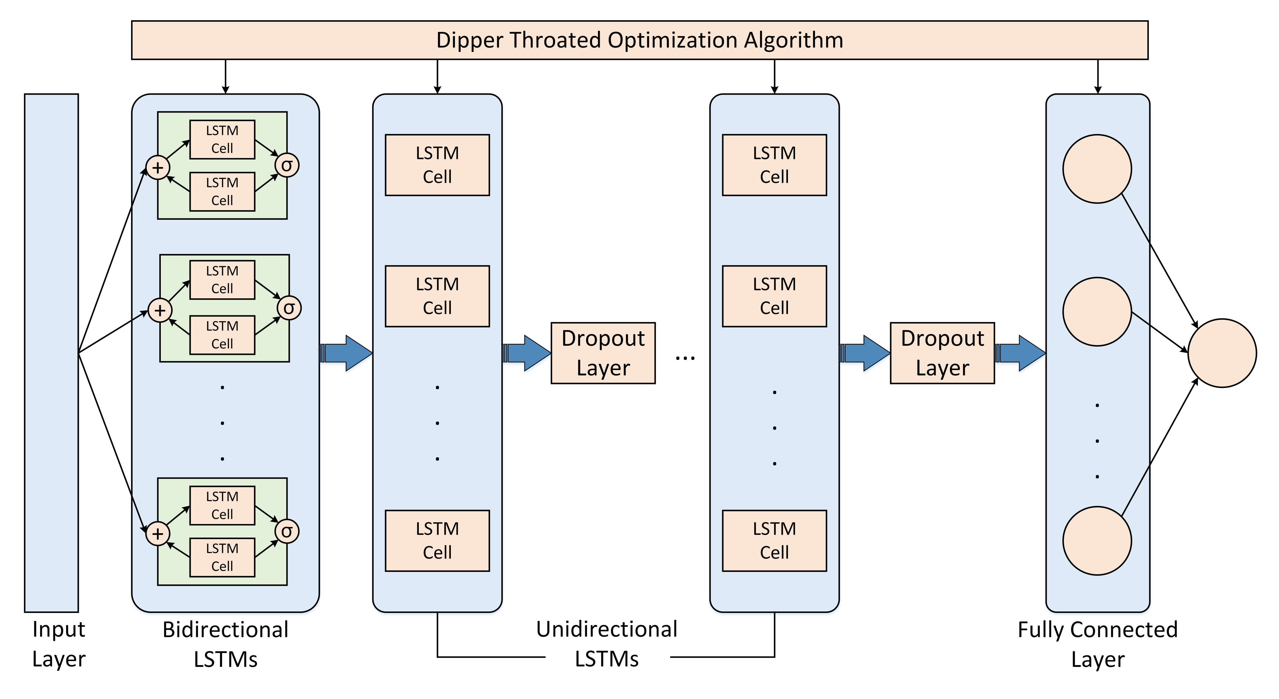
The overall architecture of the proposed optimized hybrid bidirectional and unidirectional LSTM model with fully linked dense layers is shown in Figure 4. The layers in this model fall into three categories: First, a layer composed of bidirectional LSTMs; second, layers composed of stacked unidirectional LSTMs; and third, layers composed of fully linked nodes or dense nodes. Bidirectional LSTMs, as was said before, may leverage dependencies in both directions. During the feature learning procedure, the first layer of bidirectional LSTM extracts the temporal long-term relationships of the energy consumption numbers. After gaining knowledge from the extracted all-encompassing and complicated characteristics, the next layer incorporates LSTM layers, which are effective in the forward dependencies and receives the outputs from the bottom layer. One of the most effective methods is regularizing and preventing overfitting in neural network designs by the dropout mechanism [41,42]. A dropout occurs when a portion of the neuron units are removed, along with their associated incoming and outgoing connections, resulting in a weaker network. The hybrid model has dropout layers within its stack of unidirectional LSTM layers to mitigate overfitting. Avoiding overfitting is made more accessible by early halting, leading to improved model generalization. As the last phase, we use fully connected dense layers to learn the representations retrieved up to that point, and this dense layer predicts energy use at future time steps. To effectively learn long-term dependencies and model implicit representation hidden in the sequential input, the amalgam model uses a bidirectional LSTM layer and stacks of unidirectional LSTM layers. Applications that require predictions of future energy use or loads can immediately obtain the necessary past consumption data. Therefore, there is no need to separate the use of future and historical dependencies simultaneously at any moment in time while training machine learning models.

The number of neurons of the hidden layer, the number of stacked layers, the optimization technique, the number of training iterations, and other parameters and hyperparameters of the model are all subject to optimization using the DTO algorithm. Using predefined parameters in a dictionary and their allowed values range, cross-validation with randomized search is used to conduct a search for optimal values of the parameters. In addition, the batch size refers to the total number of training samples used in a single training cycle. Batch size optimization is very important for recurrent networks such as CNN, LSTM, etc. In addition, low value to batch size has its benefits and drawbacks. Traditionally, networks can be trained more quickly using mini-batches, and a low batch size number uses less memory. However, the accuracy of the gradient estimate degrades as the batch size decreases. Initial training was carried out with a significant number for the maximum number of epochs and early stopping with the patience of 10 epochs in order to optimize the number of epochs. This approach produced a model free of overfitting and gave a rough range for the initial number of epochs.

Data Acquisition

The efficiency of the proposed model is measured by its ability to predict future electric energy usage for a collection of unique residential households. The dataset may be found in the dataset archive of the UCI Machine Learning repository [43,44]. There are 2,075,259 records in the database, and they are organized into 9 different qualities. From December 2006 to November 2010, a total of 4 years’ worth of measurements are taken at minute-by-minute intervals.

Table 1. Description of the dataset features.

No.	Features	Units	Description
1	Global active power	kW	global minute-averaged active power of a household
2	Global reactive power	kW	global minute-averaged reactive power of a household
3	Voltage	V	minute-average voltage
4	Global recurrent intensity	amps	household global minute-average current intensity
5	Sub metering 1	Wh of active energy	energy consumed by devices in the kitchen
6	Sub metering 2	Wh of active energy	energy consumed by the laundry room devices
7	Sub metering 3	Wh of active energy	energy consumed by other devices

lists the varied characteristics of the energy usage statistics. Sub metering values, active power, reactive power, and minute-average voltage and current readings are all obtainable electrical numbers. A total of 1.25% of the measurement records had no values. To account for the missing values, imputation techniques have been applied [45,46]. When feeding the raw data into the proposed model, it was first scaled using a minimum-maximum scaler, as per the following equation [47]. Scale values were set to a range from [0, 1] that covers both ends of the spectrum.

$${\widehat{x}}_m^j=\frac{x_m^j-x_{m,\mathit{min}}}{x_{m,\mathit{max}}-x_{m,\mathit{min}}}$$

(17)

where ${\widehat{x}}_m^j$ and $x_m^j$ are the normalized and raw values for feature m at time j. Maximum and lowest values for feature m that can be seen are also indicated by the notation $x_{m,\mathit{max}}$ and $x_{m,\mathit{min}}$.

It is assumed in regression models that the values for the following time step’s temperature and humidity will be available, and use these values to make predictions. Additionally, modern weather predictions have a remarkable track record of precision.

Table 2. Descriptive statistics of the dataset features.

Features	Mean	Std. Dev.	Min	Max
Global active power	1.091	1.057	0.076	11.12
Global reactive power	0.123	0.112	0.000	1.39
Voltage	240.8	3.239	223.2	254.1
Global recurrent intensity	4.627	4.444	0.200	48.40
Sub metering 1	1.121	6.153	0.000	88.00
Sub metering 2	1.298	5.822	0.000	80.00
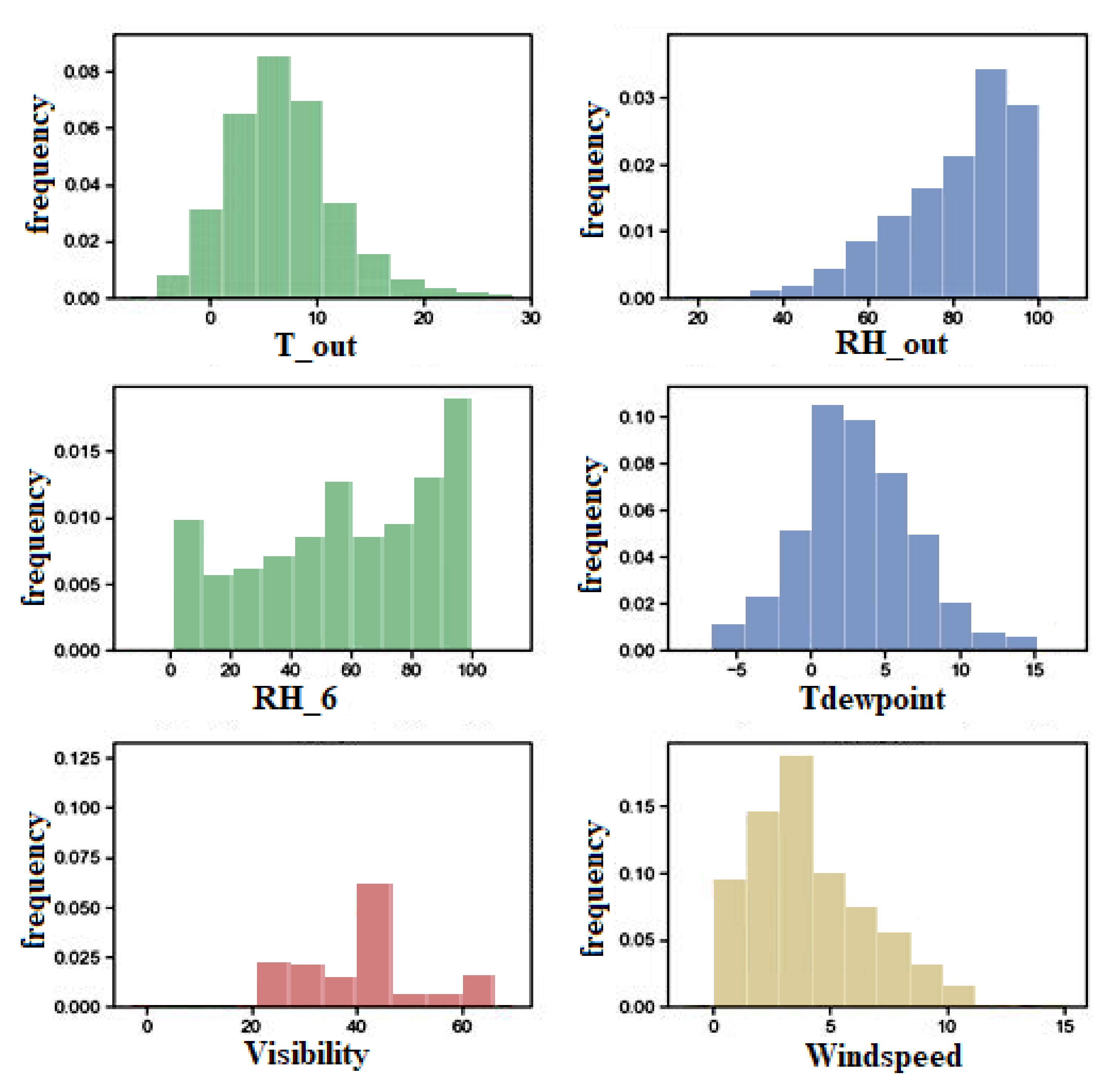
Sub metering 3	6.458	8.437	0.000	31.00

provides a summary of the descriptive statistics for the various data aspects. Variables are measured and summarized for their standard deviation, mean, maximum, and lowest values. The significant standard deviation in appliance energy use in the table further proves that energy usage in the home is very variable. Data distribution of the desired attribute, appliance energy usage, is shown in Figure 5. A long tail is a visible sign of the distribution’s significant variance. Outdoor conditions (such as wind speed, temperature, relative humidity, etc.) significantly impact the energy consumption of inside appliances. These meteorological phenomena also tend to appear in unexpected places. This is demonstrated in the plots of Figure 5 which shows the distribution of various features of the dataset.

The formulation of the forecasting of short-term energy is represented by the following formulas. Assume that the time series E provides the measurements of the energy consumption values for j time steps in the past.

$$E=e_1,e_2,e_3,\dots ,e_t,\dots ,e_j,1\le t\le j$$

(18)

Using a machine learning model denoted by f, we may predict our energy consumption at time step $t+1$ based on past consumption at time steps $t-l$ and other outdoor and interior environment variables. $e_t$ stands for the energy used during time interval t. The maximum number of time steps is j, and each time step lasts k minutes.

$$e_t=f\left(e_{1+t-l},e_{2+t-l},e_{3+t-l},\dots ,e_t,M^{t+1}\right)$$

(19)

where $M^{t+1}$ is the feature value at the $t+1$ time step (representing both the outdoor and interior environment variables).

5. Experimental Results

In this section, we provide the results of a series of experiments designed to test the efficacy of the proposed model in predicting future energy consumption in smart households and to compare the model’s results to those of several industry standards and popular machine learning approaches. SVR, KNN, Random Forest (RF), MLP, Sequence-to-Sequence (Seq2Seq), and LSTM are considered as base models in the conducted experiments. Furthermore, four optimization methods are tested and compared to the proposed approach to validate its superiority.

The experimental results were generated by running the conducted experiments on a computer with the following specifications: Core i7, 16 GB of RAM, 8 GB Nvidia RTX2070, and a Python development environment. For the training dataset, we utilized 80%, and for the test dataset, we used 20% of the full dataset. Using a k-fold cross-validation re-sampling process, we created the training and testing datasets. The value of k was determined to be 5 since this has been shown empirically to prevent excessive model bias and variation while yet providing adequate generalization [48]. Energy consumption lag values are introduced as additional features to the dataset before k-fold cross-validation is performed to account for the temporal dependencies of energy consumption on the DateTime feature. Keras (version 2.4.3), a deep learning framework, is used to configure models, with Tensor-Flow (2.2.0), an open-source software library, serving as the backend. The Keras functional Application Programming Interface (API) is used to construct the proposed model architecture.

5.1. Metrics for Performance Evaluation

The proposed approach’s performance is evaluated in terms of the metrics listed in

Table 3. List of metrics used in performance evaluation.

Metric	Value
RMSE	= $\sqrt{\frac{1}{N}{\sum }_{n=1}^N{(\widehat{V_n}-V_n)}^2}$
RRMSE	= $\frac{\mathit{RMSE}}{{\sum }_{n=1}^N\widehat{V_n}}\times 100$
MAE	= $\frac{1}{N}{\sum }_{n=1}^N|\widehat{V_n}-V_n|$
MBE	= $\frac{1}{N}{\sum }_{n=1}^N(\widehat{V_n}-V_n)$
NSE	= $1-\frac{{\sum }_{n=1}^N{(V_n-\widehat{V_n})}^2}{{\sum }_{n=1}^N{(V_n-\overline{\widehat{V_n}})}^2}$
WI	= $1-\frac{{\sum }_{n=1}^N|\widehat{V_n}-V_n|}{{\sum }_{n=1}^N|V_n-\overline{V_n}|+|\widehat{V_n}-\overline{\widehat{V_n}}|}$
$R^2$	= $1-\frac{{\sum }_{n=1}^N{(V_n-\widehat{V_n})}^2}{{\sum }_{n=1}^N{\left({\sum }_{n=1}^N{V}_n)-V_n\right)}^2}$
r	= $\frac{{\sum }_{n=1}^N(\widehat{V_n}-\overline{\widehat{V_n}})(V_n-\overline{V_n})}{\sqrt{\left({\sum }_{n=1}^N{(\widehat{V_n}-\overline{\widehat{V_n}})}^2\right)\left({\sum }_{n=1}^N{(V_n-\overline{V_n})}^2\right)}}$

. In these metrics, ($V_n$) and (${\widehat{V}}_n$) refer to the observed and estimated energy consumption. In addition, ($\overline{\widehat{V_n}}$) and ($V_n$) refer to corresponding mean values. N refers to the data points count in the dataset. The evaluation metrics employed in this work include the mean coefficient of determination ($R^2$), Mean Bias Error (MBE), Determine Agreement (WI), Root Mean Error (RMSE), Absolute Error (MAE), Pearson’s correlation coefficient (r), Relative RMSE (RRMSE), and Nash Sutcliffe Efficiency (NSE).

After preprocessing, the dataset is split into training (80%) and testing (20%). The training set is used to train the parameter optimization of the LSTM using the DTO algorithm. The parameters of the training process are set as follows. The number of populations is set to 30, the maximum number of iterations is set to 20, and the number of runs is set to 20. In addition, the same training set is used to train the other six base models for comparison purposes.

5.2. Evaluation Results

To assess the proposed approach, the criteria presented in the previous section are employed, and the results recorded by the proposed methodology are compared to those achieved by the six base models. The results and comparison are listed in

Table 4. Comparison between the proposed approach and other regression models based on the adopted evaluation criteria.

	SVR	KNN	RF	MLP	Seq2Seq	LSTM	DTO + LSTM
RMSE	0.053	0.017	0.031	0.014	0.009	0.008	0.005
RRMSE	70.56	22.05	41.01	11.19	12.59	11.19	6.232
MAE	0.053	0.011	0.026	0.013	0.008	0.006	0.003
MBE	−0.053	−0.004	−0.011	−0.012	0.001	−0.003	−0.002
NSE	0.651	0.966	0.882	0.975	0.989	0.991	0.997
WI	0.609	0.918	0.806	0.906	0.943	0.959	0.976
$R^2$	0.995	0.968	0.904	0.993	0.991	0.993	0.998
r	0.998	0.984	0.951	0.997	0.996	0.996	0.999

. In this table, the results of the proposed approach denoted by DTO + LSTM outperform those of the other models. For example, the value of the RMSE criterion achieved by the proposed approach is ($0.005$), and the value of WI is ($0.976$), which is lower than the corresponding values achieved by the other methods. Similarly, the measured criteria of the achieved results confirm the superiority of the proposed optimized model.

From the optimization algorithms perspective, the proposed approach based on the DTO algorithm is compared to four other optimization approaches. The four optimization algorithms incorporated in the conducted experiments are Particle Swarm Optimizer (PSO) [49], Genetic Algorithm (GA) [50], Grey Wolf Optimizer (GWO) [51], and Whale Optimization Algorithm (WOA) [52]. These optimizers are used to optimize the parameters of the proposed hybrid LSTM model. The statistical difference between every two methods is measured to find the p-values between the proposed DTO + LSTM method and the other methods to prove that the proposed method has a significant difference. To realize this test, Wilcoxon signed-rank test is employed. Two main hypotheses are set in this test, namely the alternate hypothesis and the null hypothesis. For the null hypothesis denoted by H0, the mean values of the algorithm are set equal ($\mu \mathit{DTO}+\mathit{LSTM}$ = $\mu \mathit{GWO}+\mathit{LSTM}$, $\mu \mathit{DTO}+\mathit{LSTM}$ = $\mu \mathit{PSO}+\mathit{LSTM}$, $\mu \mathit{DTO}+\mathit{LSTM}$ = $\mu \mathit{WOA}+\mathit{LSTM}$, $\mu \mathit{DTO}+\mathit{LSTM}$ = $\mu \mathit{GA}+\mathit{LSTM}$). Whereas in the alternate hypothesis denoted by H1, the means of the algorithms are not equal. The results of Wilcoxon’s rank-sum test are presented in

Table 5. Results of the Wilcoxon signed-rank test.

	DTO + LSTM	GWO + LSTM	PSO + LSTM	WOA + LSTM	GA + LSTM
Number of values	17	17	17	17	17
Theoretical median	0	0	0	0	0
Actual median	0.004698	0.005842	0.007731	0.008	0.006345
Sum of negative ranks	0	0	0	0	0
Sum of signed ranks (W)	153	153	153	153	153
Sum of positive ranks	153	153	153	153	153
p value (two-tailed)	<0.0001	<0.0001	<0.0001	<0.0001	<0.0001
Exact or estimate?	Exact	Exact	Exact	Exact	Exact
How big is the discrepancy?
Discrepancy	0.004698	0.005842	0.007731	0.008	0.006345
Significant (alpha = 0.05)?	Yes	Yes	Yes	Yes	Yes

. As shown in the table, the p-values are less than 0.05 when the proposed method is compared to other methods. These results confirm the superiority and statistical significance of the proposed methodology.

In addition, the one-way Analysis-of-Variance (ANOVA) test is performed to study the effectiveness of the proposed method. Similar to the Wilcoxon signed-rank test, two main hypotheses are set in this test, namely null and alternate hypotheses. For the null hypothesis denoted by H0, the mean values of the algorithm is set equal, $\mu \mathit{DTO}+\mathit{LSTM}$ = $\mu \mathit{GWO}+\mathit{LSTM}$ = $\mu \mathit{PSO}+\mathit{LSTM}$ = $\mu \mathit{WOA}+\mathit{LSTM}$ = $\mu \mathit{GA}+\mathit{LSTM}$). Whereas in the alternate hypothesis denoted by H1, the means of the algorithms are not equal. The results of the ANOVA test are listed in

Table 6. Analysis-of-variance (ANOVA) test results.

	SS	DF	MS	F (DFn, DFd)	p Value
Treatment	0.0001133	4	0.00002834	F (4, 80) = 188.6	p < 0.0001
Residual	0.00001202	80	$1.5\times {10}^{-7}$
Total	0.0001254	84

. The expected effectiveness of the proposed algorithm s confirmed when compared to the other methods based on the results of this table.

One of the first steps in doing an ANOVA is establishing the null and alternate hypotheses. Assuming there is no discernible distinction between the groups is what the null hypothesis is testing for. A significant dissimilarity between the groups is the premise of the competing hypothesis. Once the data has been cleaned, the data is checked to verify if it meets the conditions. To determine the F-ratio, they must perform the appropriate math. After this, the researcher checks the p-value against the predetermined alpha or compares the crucial value of the F-ratio with the table value. We reject the null hypothesis and accept the alternative if the estimated critical value is larger than the value in the table. In this case, we will infer that the means of the groups are unequal and reject the null hypothesis.

The descriptive analysis of the proposed approach’s prediction results of energy consumption is presented in

Table 7. Descriptive analysis of the proposed and other competing methods results.

	DTO + LSTM	GWO + LSTM	PSO + LSTM	WOA + LSTM	GA + LSTM
Number of values	17	17	17	17	17
Maximum	0.004698	0.006784	0.008731	0.008	0.007345
Median	0.004698	0.005842	0.007731	0.008	0.006345
Minimum	0.004698	0.004984	0.006731	0.006	0.005345
Mean	0.004698	0.005847	0.007672	0.00777	0.00641
Std. Error of Mean	0	0.00007725	0.000104	0.0001345	0.00009661
Std. Deviation	0	0.0003185	0.0004287	0.0005544	0.0003983
25% Percentile	0.004698	0.005842	0.007731	0.008	0.006345
75% Percentile	0.004698	0.005842	0.007731	0.008	0.006345
Range	0	0.0018	0.002	0.002	0.002
Geometric SD factor	1	1.056	1.059	1.081	1.065
Coefficient of variation	0.000%	5.447%	5.588%	7.135%	6.215%
Geometric mean	0.004698	0.005839	0.007661	0.007749	0.006398
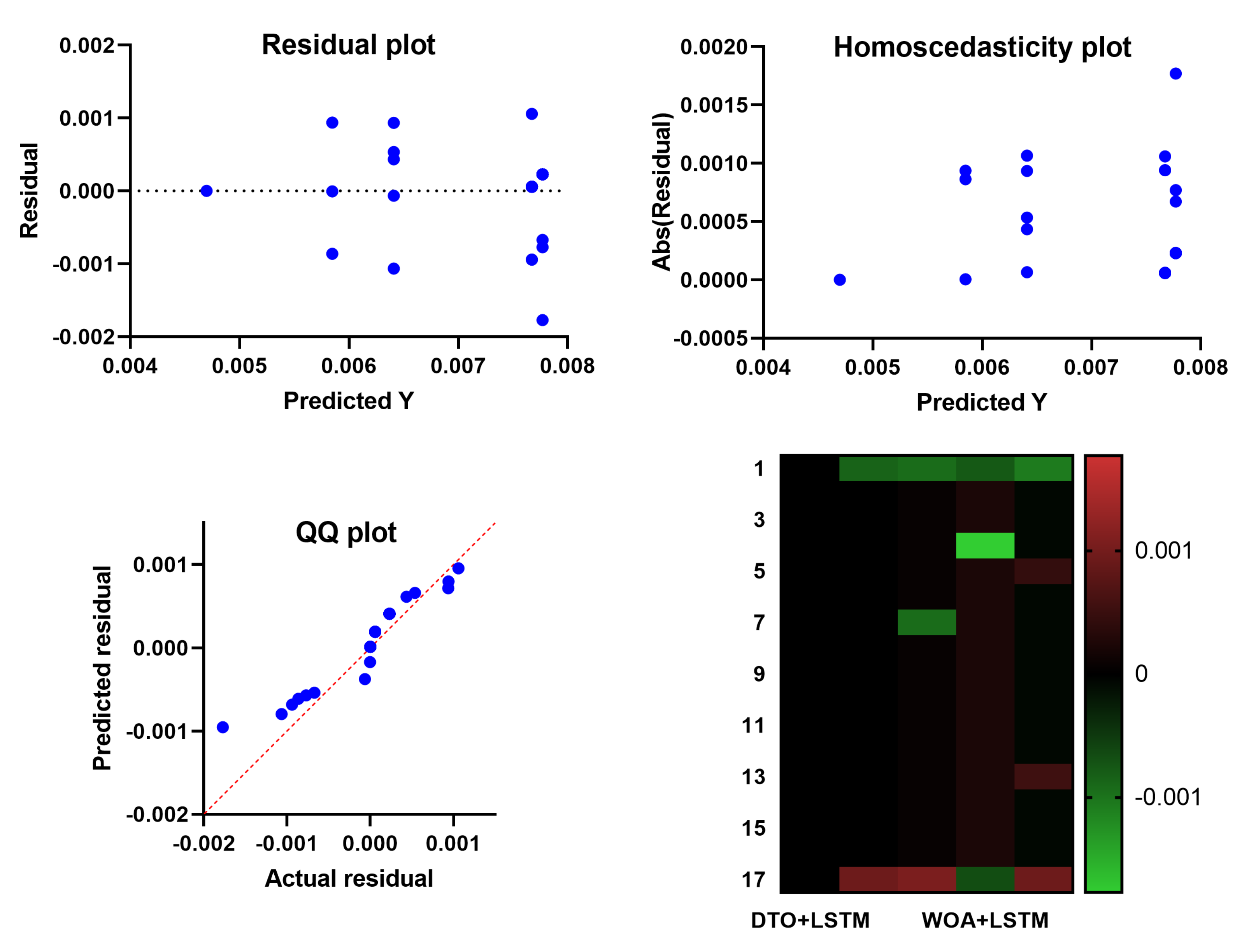
Sum	0.07987	0.0994	0.1304	0.1321	0.109

. There are 17 samples total in this table’s analysis. The proposed method is superior to the alternatives as shown by the table’s lowest, mean, maximum, and standard deviation of recorded error values. From the perspective of visual representation of the prediction results using the proposed method, Figure 6 shows four plots to illustrate the model performance. The residual plot and the homoscedasticity show the mapping between the predicted energy consumption versus the residual error. It can be noted in these plots that the residual errors are minor, which indicates the robustness of the predicted values. The QQ plot shows the fitness of the actual and predicted values. In this plot, it can be noted that the results approximately fit a straight line, proving the proposed model’s accuracy. The heatmap presented in the figure is used to show the prediction errors. In this heatmap, the proposed model gives the minimum error compared to the other approaches.

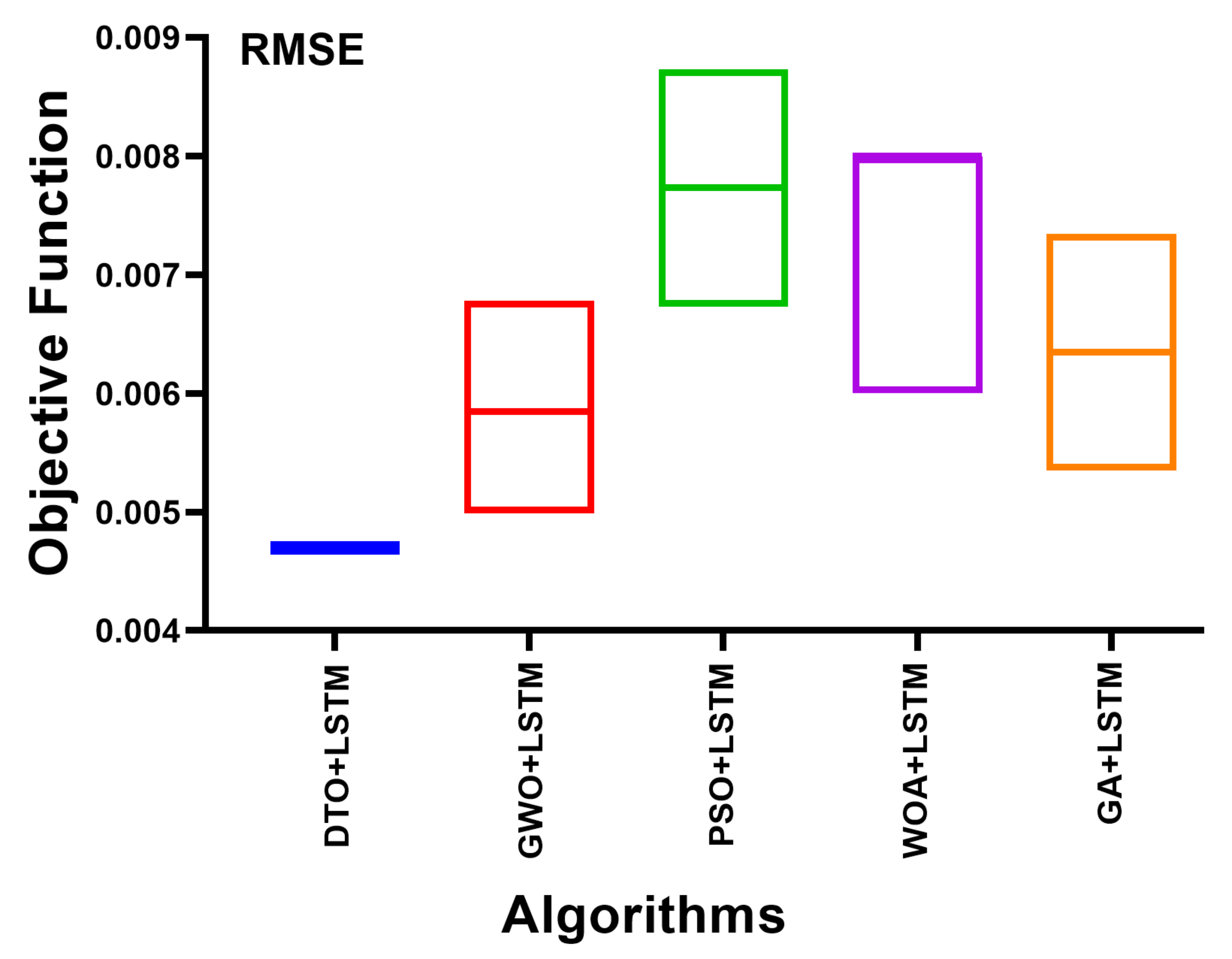
The accuracy of the power consumption forecast using the suggested method is reflected by the minimum value of Root-Mean-Square-Error (RMSE). A comparison of the RMSE between the suggested approach and the other methods is shown in Figure 7. The suggested model has the lowest RMSE values, as seen in the image. The distribution of the mistakes in the predictions is shown in a histogram in Figure 8. Compared to the other techniques, the error values of the predictions provided by the proposed model are the least, as shown in the picture. These numbers highlight the excellence of the suggested strategy in accurately estimating energy use. Figure 9 also displays the correlation between actual and expected energy usage. An illustration of the suggested method’s reliability, whereby anticipated energy usage is superimposed over observed use.

5.3. Sensitivity Analysis

Sensitivity Analysis (SA) determines how much of an impact each model parameter has on the overall system behavior. There are two types of SA, namely global and local SA. In contrast to a global analysis, which looks at sensitivity concerning the complete distribution of parameters, the local SA deals with sensitivity concerning the change of a particular parameter value. Global SA, on the other hand, analyzes the impact of input parameters on model outputs by focusing on the variance of those results. As it gives a quantitative and thorough picture of how many inputs impact the result, it is an essential tool in SA. While global SA is frequently preferable when available because of its higher information, running it on a big system is quite computationally costly. The local SA approach should be chosen when possible because it uses less processing time. In this section, we conducted a parameter-based sensitivity analysis of some parameters of the proposed DTO, namely R-parameters, exploration percentage, and C-parameters. These features are used to determine how much an algorithm can predict future energy consumption. A change can influence the optimization process in a single parameter. Therefore, a sensitivity analysis of these parameters is carried out to obtain the data that can be used to make the algorithm more effective in future iterations. The following sections present and discuss the results of three types of experiments. These experiments are one-at-a-time SA, regression analysis, and statistical significance analysis.

5.3.1. One-at-a-Time Sensitivity Analysis

We used the One-at-a-Time (OAT) sensitivity measure to carry out the sensitivity analysis [53]. The OAT method is widely regarded as one of the simplest ways to perform a sensitivity analysis. When conducting OAT, one parameter is adjusted while the others remain fixed, and the algorithm’s performance is measured in real-time. The fitness values of DTO and how they changed over time when their settings were adjusted are shown in

Table 8. Results of convergence time (in seconds) for different values of DTO’s parameters.

R-Parameter		Exploration Percentage		C-Parameter
Values	Time	Values	Time	Values	Time
0.05	6.683	5	6.587	0.1	6.701
0.10	6.475	10	7.047	0.2	6.658
0.15	6.348	15	6.772	0.3	6.592
0.20	6.833	20	6.579	0.4	6.576
0.25	6.581	25	6.378	0.5	6.632
0.30	6.444	30	6.379	0.6	6.589
0.35	6.401	35	6.374	0.7	6.619
0.40	6.390	40	6.411	0.8	6.55
0.45	6.367	45	6.369	0.9	6.615
0.50	6.371	50	6.369	1.0	6.634
0.55	6.358	55	6.389	1.1	6.589
0.60	6.367	60	6.397	1.2	6.538
0.65	6.459	65	6.388	1.3	6.608
0.70	9.671	70	6.364	1.4	6.607
0.75	9.602	75	6.371	1.5	6.556
0.80	9.412	80	6.378	1.6	6.543
0.85	7.609	85	6.372	1.7	6.548
0.90	7.900	90	6.390	1.8	6.541
0.95	6.670	95	6.388	1.9	6.525
1.00	7.124	95	6.372	2.0	6.516

and

Table 9. Results of minimization process for different values of DTO’s parameters.

R-Parameter		Exploration Percentage		C-Parameter
Values	Fitness	Values	Fitness	Values	Fitness
0.05	−18.7216	5	−16.5786	0.1	−15.5056
0.10	−18.7216	10	−16.5776	0.2	−15.5056
0.15	−19.2586	15	−18.7246	0.3	−14.4326
0.20	−19.2606	20	−18.1886	0.4	−15.5026
0.25	−18.7236	25	−18.7206	0.5	−15.5056
0.30	−18.7246	30	−18.1886	0.6	−14.4326
0.35	−18.1876	35	−18.1886	0.7	−15.5056
0.40	−18.7256	40	−18.7256	0.8	−15.5016
0.45	−18.1886	45	−18.7246	0.9	−14.4326
0.50	−18.7246	50	−17.6526	1.0	−15.5056
0.55	−18.7246	55	−18.7256	1.1	−15.5056
0.60	−19.7956	60	−19.2606	1.2	−15.5056
0.65	−18.7246	65	−18.7236	1.3	−16.5786
0.70	−18.1876	70	−18.7246	1.4	−17.6516
0.75	−18.1866	75	−18.7256	1.5	−18.7236
0.80	−19.7946	80	−18.1876	1.6	−16.5786
0.85	−18.6766	85	−19.7956	1.7	−17.6516
0.90	−19.2496	90	−18.7116	1.8	−19.7976
0.95	−19.7596	95	−18.7146	1.9	−18.7246
1.00	−19.7706	95	−19.2496	2.0	−19.7986

. Twenty values within the interval of each parameter were chosen for analysis, with additional values obtained by adding 5% to the existing interval. The algorithm was run 10 times for each variable, and the average running time and fitness are shown in the tables. The DTO algorithm is run 200 times with each parameter setting. Figure 10 shows convergent time and fitness curves for all parameters. Convergence time and fitness curves for each parameter are displayed in the figure. In terms of influencing the algorithm’s convergence time, the number of iterations and the population size were shown to be the most influential parameters. This is demonstrated by the fact that a larger population size or more iterations will result in more frequent calls to the objective function, raising the convergence time and the overall computing cost. However, with increasing vector K, the time required to converge decreases little. In addition, the algorithm’s convergence time is improved with exploration percentages over 20.

5.3.2. Regression Analysis

To learn more about how the algorithm’s parameters might account for its varying performance, a regression analysis was conducted. When we want to base our prediction of a dependent variable (the algorithm’s output) on the value of a known independent variable, regression analysis is a suitable tool (parameter). The parameters of DTO + LSTM, convergence time, and fitness were subjected to regression analysis, the results of which are presented in

Table 10. Regression analysis results for convergence time and fitness of the DTO algorithm.

	Convergence Time		Minimum Fitness
Parameters	R Square	Significance F	R Square	Significance F
R-Parameter	$5.04\times {10}^{-1}$	$2.56\times {10}^{-3}$	$8.85\times {10}^{-1}$	$6.33\times {10}^{-4}$
Exploration Percentage	$3.24\times {10}^{-1}$	$7.25\times {10}^{-5}$	$6.40\times {10}^{-1}$	$5.73\times {10}^{-3}$
C-Parameter	$2.94\times {10}^{-1}$	$4.18\times {10}^{-6}$	$6.81\times {10}^{-1}$	$6.33\times {10}^{-4}$

. How much of the overall variation in time or fitness can be accounted for by the values of the parameter is represented by the value of R Square. The greatest R Square value for convergence time is found for R-Parameter in Table 10. This suggests that this variable adequately describes the wide range of convergence times. Results from the regression model are statistically significant in predicting the algorithm’s performance, as shown in Table 10 significance F column, where values below $0.05$ indicate significance.

5.3.3. Statistical Significance Analysis

When comparing the data in Table 8 and Table 9, we wanted to see if there was a discernible difference in their respective means, so we ran an analysis of variance. Two independent analyses of variance tests were performed on the system’s convergence time and fitness values as we tweaked DTO’s parameters.

Table 11. Results of the ANOVA test for time and fitness convergence analysis of the parameters of DTO algorithm.

	SS	DF	MS	F (DFn, DFd)	p Value
Treatment	6.57	5	1.314	F (5, 114) = 24.10	p < 0.0001
Residual	6.216	114	0.05452
Total	12.79	119

shows the outcomes of an ANOVA test for the least fitness of DTO and the convergence time. p-values are less than 0.05, and F is more than F-critical, as shown in Table 11. To infer that there is a statistically significant difference between the five groups of convergence periods, we note that their averages change dramatically when the values of the parameters are changed. In addition, exploring a range of parameter values discovered a statistically significant difference in the mean values of the five subsets of least fitness. The ANOVA analysis shows no statistically significant differences between the groups. Thus, a post hoc test is executed after data from all feasible groupings have been collected. For this reason, we relied on a one-tailed t-Test with a significance level of 0.05.

Table 12. Statistical analysis of the results achieved by sensitivity analysis of DTO parameters, part 1.

	Minimum Fitness Exploration%	Convergence Time C-Parameter	Minimum Fitness C-Parameter
Actual mean	0.1705	0.3326	0.3204
Number of values	20	20	20
95% confidence interval	0.03315 to 0.3078	0.3026 to 0.3626	0.1101 to 0.5306
t, df	t = 2.598, df = 19	t = 23.24, df = 19	t = 3.189, df = 19
p value (two-tailed)	0.0177	<0.0001	0.0048
SEM of discrepancy	0.06562	0.01431	0.1004
SD of discrepancy	0.2935	0.06402	0.4492
R squared (partial eta squared)	0.2621	0.966	0.3487
Discrepancy	0.1705	0.3326	0.3204

and

Table 13. Statistical analysis of the results achieved by sensitivity analysis of DTO parameters, part 2.

	Convergence Time R-Parameter	Min. Fitness R-Parameter	Convergence Time Exploration%
Actual mean	0.5998	0.89	0.3888
Number of values	20	20	20
95% confidence interval	0.5355 to 0.6641	0.8795 to 0.9005	0.3300 to 0.4475
t, df	t = 19.54, df = 19	t = 178.0, df = 19	t = 13.85, df = 19
p value (two-tailed)	<0.0001	<0.0001	<0.0001
SEM of discrepancy	0.0307	0.005	0.02808
SD of discrepancy	0.1373	0.02236	0.1256
R squared (partial eta squared)	0.9526	0.9994	0.9098
Discrepancy	0.5998	0.89	0.3888

illustrate the outcomes of a t-Test conducted on each set of parameters, including the convergence time and minimal fitness of DTO, respectively. In the table, p-values below 0.05 indicate statistically significant differences between the groups. The p-value for convergence time is greater than 0.05 according to the t-Test comparing the proportion of time spent investigating and the percentage of time spent evolving. The sensitivity analysis, however, is graphically shown in Figure 11. The residual and homoscedasticity plots, as well as the QQ and heatmap plots, all exhibit minimum values between the residual and the projected values, demonstrating the stability of the proposed methodology. The proposed approach is shown to be resilient via the QQ and heatmap plots, which remain accurate even after varying some of the input values.

5.4. Linear Regression Analysis

The standardized residual quantifies the extent to which actual data deviates from predicted results. In relation to the chi-square value, it indicates the relative importance of the results. Using the standardized residual, it can be easily shown which results are making the most and smallest contributions to the total value. In this work, linear regression analysis is used to compare the results of the proposed approach and the other approaches to detect the outliers. Figure 12 shows the regression analysis plot. In this plot, it can be noted that the residual values are tiny, and thus indicates no outliers. In addition,

Table 14. Results of the linear regression analysis applied to the proposed approach records and compared to the other four competing approaches.

Linear Regression	GWO + LSTM	PSO + LSTM	WOA + LSTM	GA + LSTM
Std. Error
Slope	0.01644	0.02213	0.02862	0.02056
Best-fit values
Slope	1.245	1.633	1.654	1.364
1/slope	0.8035	0.6123	0.6046	0.733
Y-intercept
95% Confidence Intervals
Slope	1.210 to 1.279	1.586 to 1.680	1.593 to 1.715	1.321 to 1.408
Y-intercept	0.000 to 0.000	0.000 to 0.000	0.000 to 0.000	0.000 to 0.000
X-intercept	−infinity to +infinity	−infinity to +infinity	−infinity to +infinity	−infinity to +infinity
Data
Total number of values	17	17	17	17
Number of X values	17	17	17	17
Maximum number of Y replicates	1	1	1	1
Z-Score	0.557186	0.557186	0.557186	0.557186
Number of missing values	0	0	0	0
Goodness of Fit
Sy.x	0.0003185	0.0004287	0.0005544	0.0003983
F	5729	5444	3340	4402
DFn, DFd	1, 16	1, 16	1, 16	1, 16
Deviation from zero?	Significant	Significant	Significant	Significant
Equation	Y = 1.245*X + 0.000	Y = 1.633*X + 0.000	Y = 1.654*X + 0.000	Y = 1.364*X + 0.000
p-value	<0.0001	<0.0001	<0.0001	<0.0001

presents the detailed results of the linear regression analysis. In this table, it can be noted that the p-value is less than 0.05 and the value of the z-score is greater than 0.5 which also proves the significance of the proposed approach with no outliers.

6. Conclusions

Increased precision in building-level energy consumption forecasting has significant implications for energy resource development and scheduling and for making the most of renewable energy sources. To improve the accuracy with which energy consumption can be predicted, this research proposed a novel approach based on an optimized hybrid deep learning model that combines the benefits of traditional unidirectional LSTMs and bidirectional LSTMs. The optimization of this deep learning model is performed in terms of the DTO algorithm. The bidirectional LSTMs are employed to accurately predict future energy consumption levels by recognizing underlying trends in energy use. To test the effectiveness of the suggested methodology, we used data on smart home energy use. The proposed model has also been compared against several other regression models and optimization methods, including the SVR, KNN, RF, MLP, Seq2Seq, and LSTM, as well as the GWO, WOA, PSO, and GA algorithms. The findings demonstrated the large gains made by the suggested method compared to the benchmark regression models. The robustness of the proposed method is evaluated using statistical analysis, with results highlighting the anticipated outcomes. The proposed optimization method’s optimization parameters’ relevance is further demonstrated by sensitivity analysis. The experimental findings showed that the proposed method was superior to the alternatives, with RMSE of 0.0047 and $R^2$ of 0.998, respectively. The study’s long-term goals include testing the proposed method’s scalability by applying it to bigger datasets with various use cases.