Robust Output Feedback Control of the Voltage Source Inverter in an AC Microgrid

Abstract

This paper presents the mathematical model and control of the voltage source inverter (VSI) connected to an alternating current (AC) microgrid. The VSI used in this work was a six-switch three-phase PWM inverter, whose output voltages were controlled in a synchronous ($dq$) reference frame via a sliding mode control strategy. The control strategy required only output voltages; other states of the system were estimated by using a high-gain observer. The power-sharing among multiple inverters was achieved by solving power flow equations of the electrical network. The stability analysis showed that the error was ultimately bound in the case of the real PWM inverter and/or with a nonlinear load in the electrical network. The microgrid was simulated using the SimPowerSystems Toolbox from MATLAB/Simulink. The simulation results show the effectiveness of the proposed control scheme. The output voltage regulation of the inverter and power-sharing was achieved with the ultimately bounded error for the linear load. Later, the nonlinear load was also included in the electrical network and the error was shown to remain ultimately bounded. The output voltage regulation and power-sharing were achieved with the nonlinear load in the system.

1. Introduction

The conventional electrical grid is a vast network, composed of large electricity generating systems, multiple transformers, transmission lines, and distribution lines. The distance between electricity generation and electricity consumption is large (100 s of Km). Due to these distances, the line losses are huge and any failures in the transmission lines can cause a disruption of electricity for a large population. The solution lies in the microgrid [1]. The microgrid is a low voltage electricity grid that works at the distribution level. It is composed of small electricity generation systems (such as solar-based generation and wind-based generation) distributed over the network and electrical loads at the distribution level [2,3]. These generating systems are called distributed generating units (DG units). The integration of DG units at the distribution level poses multiple challenges that need to be solved [4]. The DG units are connected to the microgrid through voltage source inverter (VSIs) [5]. For the operation of the microgrid, proper control system mechanisms are required to stabilize the voltage and frequency of the inverters and to perform proper power-sharing among multiple DG units [6]. VSIs can work in the voltage control mode (VCM) or in power control mode (PCM) [7]. The microgrid operates in the grid-connected mode or in the islanded mode [8,9]. Under the grid-connected mode, the voltage and frequency of the microgrid are determined by the main grid. Microgrid control systems work in the PCM, perform active and reactive power-sharing among the DG units, and exchange power with the main grid [10]. In the islanded mode, at least one VSI must work in the VCM [7]. In the VCM, the control system of the inverter must stabilize the output voltage magnitude, frequency, and phase. It must also maintain the sinusoidal shape of the inverter output [11]. The control system of the VSI must work with the presence of any unknown load. The unknown load means unknown disturbance, so the control system must be able to reject any kind of disturbances. The DG units frequently join and leave the microgrid, resulting in the change of grid topology, so the control system must be able to work in a distributed way and only depend on the variables, which are locally available [12]. The control system of the VSI can be designed in a natural ($abc$) reference frame, a stationary ($\alpha \beta$) reference frame, or a synchronous ($dq$) reference frame [13]. The AC voltage and current signals appear as sinusoidal in the $abc$ and $\alpha \beta$ reference frames but as constants in the $dq$ reference frame. These signals can be converted using Clarke and Park transformations [14]. Control systems designed in the $abc$ or $\alpha \beta$ reference frames track their sinusoidal reference signals, whereas control systems designed in the $dq$ reference frame track the constant reference signals.

This paper focuses on the control system design of the VSI in the voltage control mode (VCM). Many control system designs have been proposed in the literature on this problem. PI controllers [15] are employed in the cascaded configuration as current and voltage controllers. The structure of the controller is simple; however, the parameters of the controller are difficult to tune. The LC filter of the VSI introduces oscillatory behavior in the output if the parameters of the controller are not perfectly tuned [16]. PI controllers with automatic tuning of controller gains have also been introduced in the literature. A self-adaptive Salp Swarm optimization-based tuning of the PI controller was applied for microgrid control [17]. A hybrid Harris hawks and particle swarm optimization algorithm (H-HHOPSO)-based tuning of the PI controller was given for the microgrid control [18]. The PI control was applied in the $dq$ reference frame. PR controllers [19,20,21] have also been applied to the microgrid control. PR controllers were applied in $\alpha \beta$ and $abc$ reference frames, tracking sinusoidal reference signals.

Optimal control techniques have been applied in the microgrid control. These techniques work on optimizing some objective functions or minimizing some cost functions. In reference [22], the authors applied optimal control to regulate the output voltage and power-sharing by solving a constrained optimization problem. A convex optimization problem with the involvement of linear matrix inequalities was solved to synthesize the voltage controller of the inverter in the microgrid [23]. A model-based optimal linear quadratic tracking control [24] was applied to regulate the voltage and current control of the AC microgrid with optimally-minimizing system energy. Joint control of the linear quadratic optimal control and disturbance residual generator [25] was applied for the output voltage control of the inverter in the AC microgrid with disturbance observation and cancellation. Model predictive control [26,27,28] was applied to the microgrid control; however, it required the exact information of the model and parameters. MPC works by predicting the plant output over a prediction horizon and finding the appropriate control signal over a control horizon by solving a constrained optimization problem. It lacks the robustness to disturbances and parametric uncertainty. In [29], the authors provide a detailed review of the model predictive control applied on the microgrid.

$H_2$ control is another optimal control technique that finds the controller by minimizing a cost function based on the $H_2$ norm. It has been applied in the microgrids to improve the transient performance in the output voltage of the inverter, but it lacks the robustness to disturbance and parametric variations [30]. Due to disturbances and parametric uncertainties, a robust control strategy is required that ensures stability in worst-case scenarios. Robust $H_{\infty }$ controllers [31,32,33,34,35] have been applied and ensure stability in the presence of parametric uncertainties. In the $H_{\infty }$ control, the controller is also synthesized by solving an optimization problem. A $H_{\infty }$ norm-based cost function is minimized. $H_{\infty }$ control with an artificial bee colony algorithm [36] has been applied for voltage and frequency control with power-sharing among multiple inverters in the microgrid. Mixed $H_2/H_{\infty }$ controllers [37,38,39] have been applied as well to provide robust stability in the presence of parametric uncertainties and disturbances. A mixed $H_2/H_{\infty }$ control with Markov chain [40] has been applied to regulate frequency and energy sharing in the microgrid. A robust $\mathsf{\mu }$-synthesis controller [41] was designed to regulate the output voltage of the inverter and power-sharing among multiple inverters in an AC microgrid. It is an output feedback controller (thus, removing the requirement for any other state of the system). It also provides the damping of resonant oscillations and robustness to control loop delays and parametric uncertainties.

In addition to linear controls, nonlinear control strategies, such as sliding mode controllers [38,42,43,44,45,46], have been applied, ensuring robust stability in worst-case scenarios of disturbances and parametric variations. Intelligent control techniques have been applied as well, but require training procedures (and the tuning of training parameters is difficult). Adaptive fuzzy control [47] has been applied for microgrid voltage control. Neural network and fuzzy logic-based control schemes [48] have been applied for microgrid voltage control and energy management. In [49], the authors provide a detailed review of various neural network algorithms applied to the AC microgrid. In [50], the authors provide the current progress and future scopes for the implementation of artificial intelligence techniques in the microgrid control. In a microgrid, all voltage controllers need a synchronization signal, which is provided by a global positioning system (GPS) [51].

In this paper, a high-gain observer (HGO)-based sliding mode controller (SMC) is presented for VSI control in the VCM. The power-sharing among multiple inverters was achieved by solving power flow equations [52] for a microgrid. The main contribution of the paper is the SMC design and its stability analysis for the problem of the VSI output voltage control in the $dq$ reference frame. SMC is a robust control scheme that provides the stability for the worst-case scenario of perturbation in system variables, system parameters, and disturbance signals. The use of this controller for VSI in the microgrid shows that if the possible variations in electrical parameters are known, a controller with robust stability can be designed. Furthermore, HGO and its stability analysis are presented for state estimation. HGO saves the requirement of two three-phase current sensors and only a three-phase voltage sensor is required for the control scheme. HGO also provides state feedback performance with the output feedback control [53].

A mathematical model of the microgrid and control problem is presented in Section 2. The control scheme is presented in Section 3. Section 4 presents the stability analysis. Power-sharing is discussed in Section 5. The simulation results are presented in Section 6. The paper is concluded in Section 7.

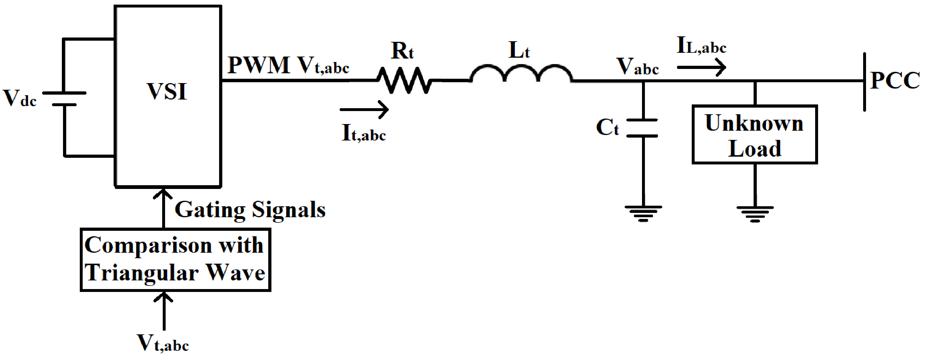
2. Problem Formulation

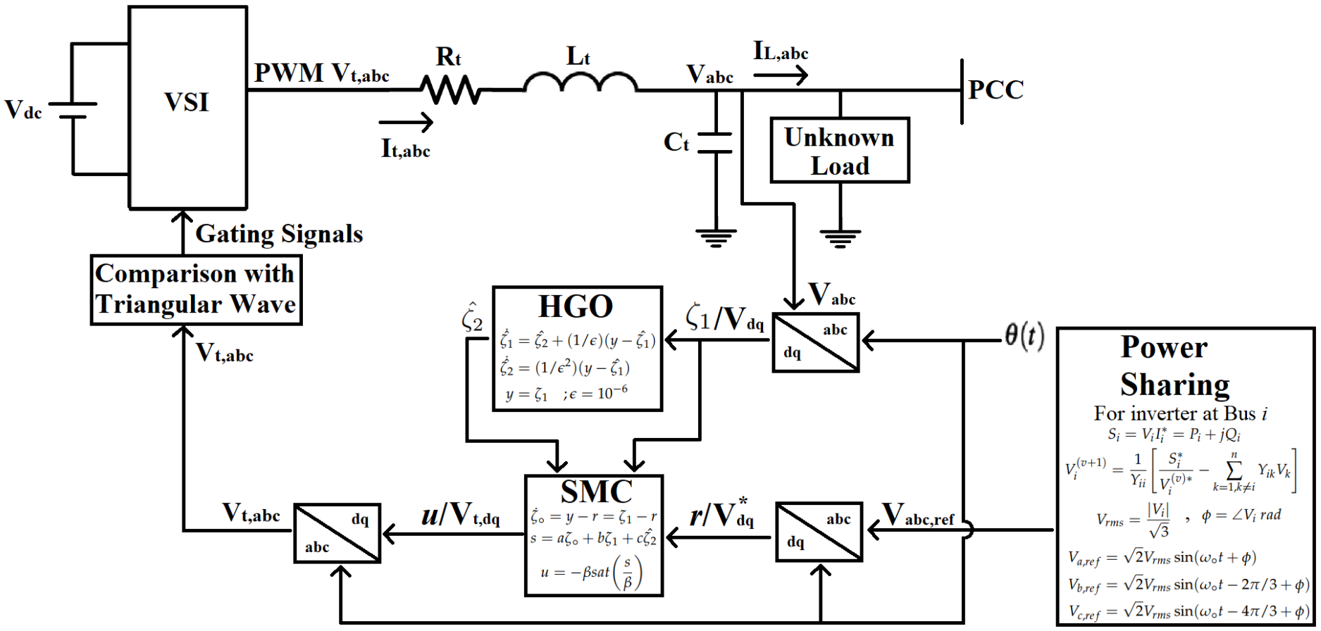
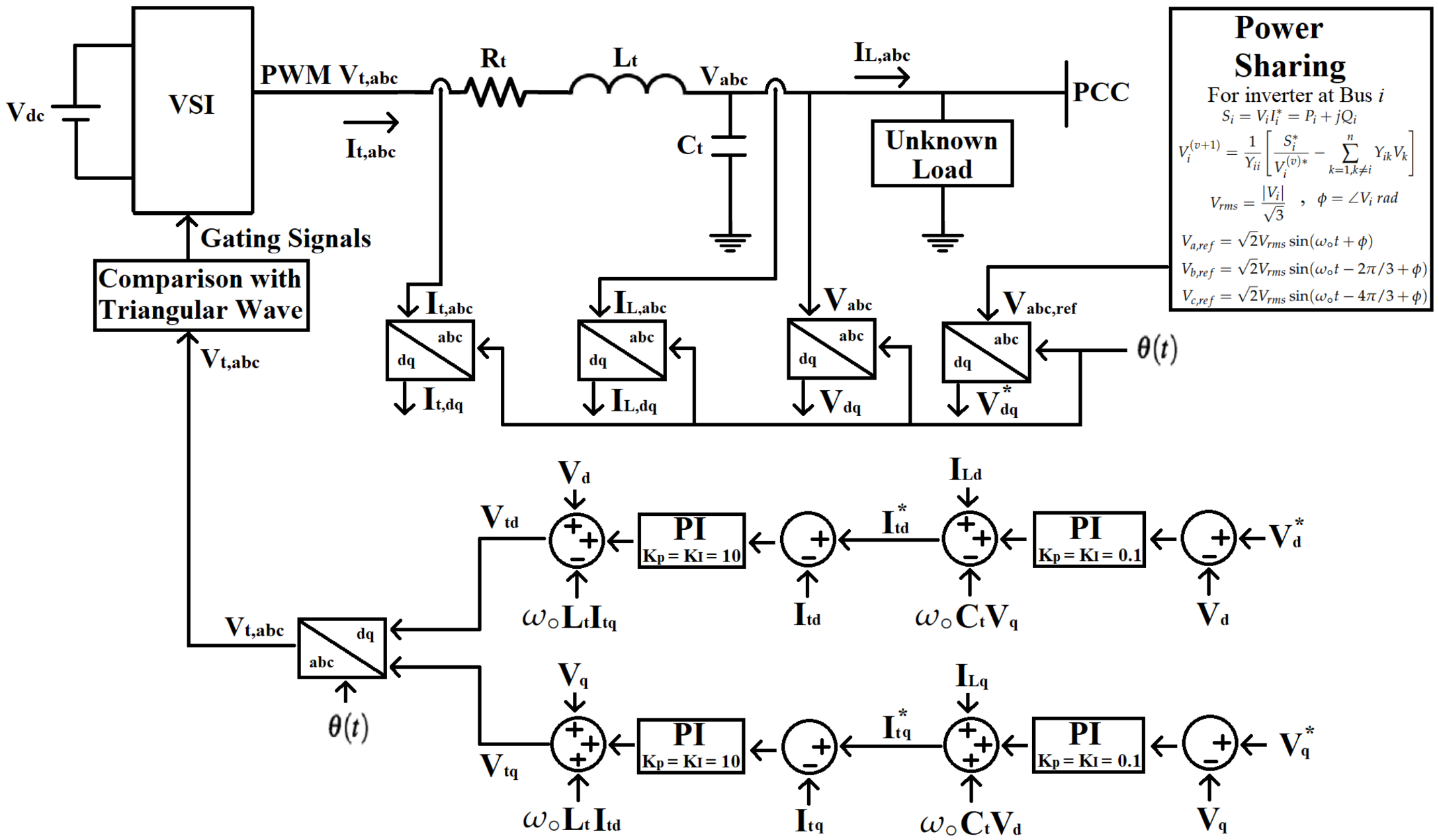
In a microgrid, DG units are connected through the VSI. The VSI used here is a PWM inverter, which requires an $RLC$ filter at the output to extract the fundamental frequency from the generated PWM voltage signal. The VSI with its output filter is shown in Figure 1. In this figure, ${\mathbf{V}}_{\mathbf{t},\mathbf{abc}}$ is the VSI terminal voltage, ${\mathbf{I}}_{\mathbf{t},\mathbf{abc}}$ is the filter current, ${\mathbf{V}}_{\mathbf{abc}}$ is the output voltage, and ${\mathbf{I}}_{\mathbf{L},\mathbf{abc}}$ is the load current or current injected into the microgrid by the VSI. $R_t$, $L_t$, and $C_t$ are the resistance, inductance, and capacitance of the VSI output filter, respectively. The inverter was connected to the microgrid at the point of common coupling (PCC).

The problem considered in this paper was voltage control at the PCC. For the control design, a mathematical model of the system shown in Figure 1 was required. So, without considering the switching phenomenon of the PWM inverter, the system shown in Figure 1 can be represented by the following dynamical equations in the $abc$ reference frame [31].

$$\begin{array}{cc}\hfill {\mathbf{V}}_{\mathbf{t},\mathbf{abc}}& =L_t\frac{d{\mathbf{I}}_{\mathbf{t},\mathbf{abc}}}{d_t}+R_t{\mathbf{I}}_{\mathbf{t},\mathbf{abc}}+{\mathbf{V}}_{\mathbf{abc}}\hfill \\ \hfill {\mathbf{I}}_{\mathbf{t},\mathbf{abc}}& ={\mathbf{I}}_{\mathbf{L},\mathbf{abc}}+C_t\frac{d{\mathbf{V}}_{\mathbf{abc}}}{d_t}\hfill \end{array}$$

(1)

Here, ${\mathbf{V}}_{\mathbf{t},\mathbf{abc}}$, ${\mathbf{I}}_{\mathbf{t},\mathbf{abc}}$, ${\mathbf{V}}_{\mathbf{abc}}$ and ${\mathbf{I}}_{\mathbf{L},\mathbf{abc}}$ are $3\times 1$ vectors, representing the three-phase signals. The system can also be represented in the $dq$ reference frame by the following dynamical equations.

$$\begin{array}{cc}\hfill \frac{d{V}_d}{dt}& ={\omega }_{\circ }{V}_q+\frac{1}{C_t}{I}_{td}-\frac{1}{C_t}{I}_{Ld}\hfill \\ \hfill \frac{d{I}_{td}}{dt}& =\frac{1}{L_t}{V}_{td}-\frac{R_t}{L_t}{I}_{td}-\frac{1}{L_t}{V}_d+{\omega }_{\circ }{I}_{tq}\hfill \\ \hfill \frac{d{V}_q}{dt}& =-{\omega }_{\circ }{V}_d+\frac{1}{C_t}{I}_{tq}-\frac{1}{C_t}{I}_{Lq}\hfill \\ \hfill \frac{d{I}_{tq}}{dt}& =\frac{1}{L_t}{V}_{tq}-\frac{R_t}{L_t}{I}_{tq}-\frac{1}{L_t}{V}_q-{\omega }_{\circ }{I}_{td}\hfill \end{array}$$

(2)

Here, ${\omega }_{\circ }$ is the angular frequency of the system. The variables in Equation (2) are linked with variables in Equation (1) by Park’s transformation, as follows:

$$\begin{array}{c}{\mathbf{V}}_{\mathrm{a}\mathrm{b}\mathrm{c}}⟷V_d,V_q\hfill \\ {\mathbf{V}}_{\mathrm{t},\mathrm{a}\mathrm{b}\mathrm{c}}⟷V_{td},V_{tq}\hfill \\ {\mathbf{I}}_{\mathrm{t},\mathrm{a}\mathrm{b}\mathrm{c}}⟷I_{td},I_{tq}\hfill \\ {\mathbf{I}}_{\mathrm{L},\mathrm{a}\mathrm{b}\mathrm{c}}⟷I_{Ld},I_{Lq}\hfill \\ {\mathbf{V}}_{\mathrm{a}\mathrm{b}\mathrm{c},\mathrm{r}\mathrm{e}\mathrm{f}}⟷V_d^{\ast },V_q^{\ast }\hfill \end{array}$$

Here, ${\mathbf{V}}_{\mathbf{abc},\mathbf{ref}}$ is defined as:

$$\begin{array}{cc}\hfill V_{a,ref}& =\sqrt{2}{V}_{rms}sin({\omega }_{\circ }t+\varphi )\hfill \\ \hfill V_{b,ref}& =\sqrt{2}{V}_{rms}sin({\omega }_{\circ }t-2\pi /3+\varphi )\hfill \\ \hfill V_{c,ref}& =\sqrt{2}{V}_{rms}sin({\omega }_{\circ }t-4\pi /3+\varphi )\hfill \end{array}$$

(3)

$V_{rms}$ and $\varphi$ in Equation (3) will be generated from the power-sharing mechanism.

The sinusoidal signals in the $abc$ reference frame appear as step signals in the $dq$ reference frame. So, the problem considered in this paper was to design a control scheme in the $dq$ reference frame, capable of minimizing the following tracking errors to an ultimate bound in finite time, by manipulating the variables $V_{td}$ and $V_{tq}$. Moreover, $V_{td}$ and $V_{tq}$ are control signals to be generated by the control scheme; these signals will be converted into the $abc$ reference frame to generate the gating signals of the VSI.

$$\begin{array}{cc}\hfill e_d& =V_d-V_d^{\ast }\hfill \\ \hfill e_q& =V_q-V_q^{\ast }\hfill \end{array}$$

(4)

3. Control Scheme

In this section, the sliding mode control is presented to regulate the output voltage of the VSI in the $dq$ reference frame. The control design is model-based and a mathematical model of the VSI in the $dq$ reference frame was used, which is given in Equation (2). The system shown in Equation (2) is a multiple-input multiple-output system with two inputs $\left\{V_{td},V_{tq}\right\}$ and two outputs $\left\{V_d,V_q\right\}$. This system can be converted into two single-input single-output systems by considering the following change of variables so that two separate controllers can be designed with a single input and a single output.

$$\begin{gathered} x_{1d}=V_d,x_{2d}=I_{td},u_d=V_{td},y_d=V_d,r_d=V_d^{\ast }, \\ {d}_{1d}=-I_{Ld}+{\omega }_{\circ }{C}_t{V}_q,d_{2d}={\omega }_{\circ }{I}_{tq} \end{gathered}$$

and

$$\begin{gathered} x_{1q}=V_q,x_{2q}=I_{tq},u_q=V_{tq},y_q=V_q,r_q=V_q^{\ast }, \\ {d}_{1q}=-I_{Lq}-{\omega }_{\circ }{C}_t{V}_d,d_{2q}=-{\omega }_{\circ }{I}_{td} \end{gathered}$$

The two single-input single-output systems are as follows:

$$\begin{array}{cc}\hfill {\dot{x}}_{1j}& =\frac{1}{C_t}{x}_{2j}+\frac{1}{C_t}{d}_{1j}\hfill \\ \hfill {\dot{x}}_{2j}& =-\frac{1}{L_t}{x}_{1j}-\frac{R_t}{L_t}{x}_{2j}+\frac{1}{L_t}{u}_j+d_{2j}\hfill \\ \hfill y_j& =x_{1j}\hfill \end{array}$$

(5)

here, $j=d,q$.

Here, one system is with $j=d$ and the other system is with $j=q$. Both of these systems are second-order linear time-invariant systems. Here, $x_{1j}$ and $x_{2j}$ are state variables, $u_j$ is the input variable, $y_j$ is the output variable, $d_{1j}$ and $d_{2j}$ are disturbance variables, and $r_j$ is the reference signal.

Equation (5) clearly suggests that both systems contain the same dynamics and the same controller can be designed for both systems. From this point, j will be dropped from Equation (5) for the controller design.

The system shown in Equation (5) is in x coordinates. It can be converted into normal form ($\zeta$ coordinates) by considering the following change of variables. The normal form is useful in the control design.

$$\begin{array}{cc}\hfill {\zeta }_1& =x_1\hfill \\ \hfill {\zeta }_2& =\frac{1}{C_t}{x}_2+\frac{1}{C_t}{d}_1\hfill \end{array}$$

The system in the $\zeta$ coordinates is as follows:

$$\begin{array}{cc}\hfill {\dot{\zeta }}_1& ={\zeta }_2\hfill \\ \hfill {\dot{\zeta }}_2& =-\frac{1}{L_t{C}_t}{\zeta }_1-\frac{R_t}{L_t}{\zeta }_2+\frac{R_t}{L_t{C}_t}{d}_1+\frac{1}{C_t}{d}_2\hfill \\ \hfill & \phantom{=}+\frac{1}{C_t}{\dot{d}}_1+\frac{1}{L_t{C}_t}u\hfill \\ \hfill {\dot{\zeta }}_2& =h(\zeta ,d_1,d_2)+gu\hfill \\ \hfill y& ={\zeta }_1\hfill \end{array}$$

(6)

In this paper, based on the system shown in Equation (6), the sliding mode controller [54] is designed with the following sliding surface ‘s’ shown in Equation (7),

$$s=a{\zeta }_{\circ }+b{\zeta }_1+c{\zeta }_2;{\dot{\zeta }}_{\circ }=y-r={\zeta }_1-r$$

(7)

Using the sliding surface ‘s’, the controller equation is given as follows in Equation (8). In the controller equation, $\beta$ is a constant that must satisfy the inequality given in Equation (8).

$$u=-\beta sat\left(\frac{s}{\beta }\right);\beta \ge \rho (\zeta ,d_1,d_2)+{\beta }_{\circ },{\beta }_{\circ }>0$$

(8)

The $\beta$ value depends on $\rho (\zeta ,d_1,d_2)$; this $\rho (\zeta ,d_1,d_2)$ value can be found as follows by using inequality (9).

$$\begin{array}{cc}\hfill \dot{s}& =a{\dot{\zeta }}_{\circ }+b{\dot{\zeta }}_1+c{\dot{\zeta }}_2\hfill \\ \hfill \dot{s}& =a({\zeta }_1-r)+b{\zeta }_2+c[h(\zeta ,d_1,d_2)+gu]\hfill \end{array}$$

$$\left|\frac{a({\zeta }_1-r)+b{\zeta }_2+ch(\zeta ,d_1,d_2)}{cg}\right|\le \rho (\zeta ,d_1,d_2)$$

(9)

The bounds on variables and constants involved in inequality (9) can be found by the electrical characteristics of the VSI. These bounds on variables and constants represent the worst-case scenarios of perturbation in the system parameters, system variables, and disturbance signals. Thus, by following the inequality (9), a robust controller is designed for this worst-case scenario.

The values of a, b, and c in the sliding surface Equation (7) can be found as follows. As shown in Equation (8), when $\left|s\right|\le \beta$, $u=-s$.

$$\begin{array}{cc}\hfill u& =\mathbf{F}{\left[{\zeta }_{\circ }{\zeta }_1{\zeta }_2\right]}^T;\mathbf{F}=[-a-b-c]\hfill \end{array}$$

(10)

Consider the following system:

$$\begin{array}{cc}\hfill \dot{\zeta }& =\mathbf{A}\zeta +\mathbf{B}u\hfill \\ \hfill \left[\begin{array}{c}{\dot{\zeta }}_{\circ }\\ {\dot{\zeta }}_1\\ {\dot{\zeta }}_2\end{array}\right]& =\left[\begin{array}{ccc}0& 1& 0\\ 0& 0& 1\\ 0& \frac{-1}{L_t{C}_t}& \frac{-R_t}{L_t}\end{array}\right]\left[\begin{array}{c}{\zeta }_{\circ }\\ {\zeta }_1\\ {\zeta }_2\end{array}\right]+\left[\begin{array}{c}0\\ 0\\ \frac{1}{L_t{C}_t}\end{array}\right]u\hfill \end{array}$$

(11)

$\mathbf{F}$ can be found by any feedback design method that stabilizes the system shown in Equation (11) with controller Equation (10) (i.e., the $\mathbf{A}+\mathbf{BF}$ matrix has all eigenvalues with a negative real part) and achieves the desired transient response.

The designed controller needs two variables ${\zeta }_1$ and ${\zeta }_2$, which require a three-phase voltage sensor and two three-phase current sensors. To save the sensors, ${\hat{\zeta }}_2$ is used instead of ${\zeta }_2$ by using the high-gain observer (HGO) [54,55]. This saves the requirement of two three-phase current sensors and only a three-phase voltage sensor is now required. The HGO is given as follows:

$$\begin{array}{cc}\hfill \dot{\widehat{{\zeta }_1}}& =\widehat{{\zeta }_2}+(1/ϵ)(y-\widehat{{\zeta }_1})\hfill \\ \hfill \dot{\widehat{{\zeta }_2}}& =(1/{ϵ}^2)(y-\widehat{{\zeta }_1})\hfill \\ \hfill y& ={\zeta }_1;ϵ={10}^{-6}\hfill \end{array}$$

(12)

The controller with HGO only requires output voltages $\left\{V_d,V_q\right\}$ to generate control signals $\left\{V_{td},V_{tq}\right\}$. The complete control scheme is also shown in Figure 2.

4. Stability Analysis

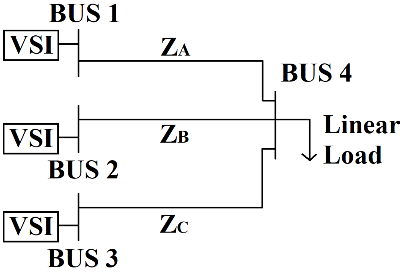
For the system in Equation (6) and the designed controller in Equation (8), the stability analysis [54] is given as follows.

Considering the following positive definite Lyapunov function V and its derivative $\dot{V}$, the stability analysis is shown for the values of ‘s’ outside the boundary layer ($\left|s\right|>\beta$).

$$\begin{array}{cc}\hfill V& =\frac{1}{2}{s}^2\hfill \\ \hfill \dot{V}& =s\dot{s}\hfill \\ \hfill \dot{V}& =s[a({\zeta }_1-r)+b{\zeta }_2+ch(\zeta ,d_1,d_2)]+scgu\hfill \\ \hfill \dot{V}& \le \left|s\right|cg\rho (\zeta ,d_1,d_2)+scgu\hfill \end{array}$$

For $s>\beta ,u=-\beta$

$$\begin{array}{cc}\hfill \dot{V}& \le \left|s\right|cg\rho (\zeta ,d_1,d_2)-\left|s\right|cg\beta \hfill \\ \hfill \dot{V}& \le \left|s\right|cg\rho (\zeta ,d_1,d_2)-\left|s\right|cg[\rho (\zeta ,d_1,d_2)+{\beta }_{\circ }]\hfill \\ \hfill \dot{V}& \le -cg{\beta }_{\circ }\left|s\right|<0\hfill \end{array}$$

For $s<-\beta ,u=\beta$

$$\begin{array}{cc}\hfill \dot{V}& \le \left|s\right|cg\rho (\zeta ,d_1,d_2)-\left|s\right|cg\beta \hfill \\ \hfill \dot{V}& \le \left|s\right|cg\rho (\zeta ,d_1,d_2)-\left|s\right|cg[\rho (\zeta ,d_1,d_2)+{\beta }_{\circ }]\hfill \\ \hfill \dot{V}& \le -cg{\beta }_{\circ }\left|s\right|<0\hfill \end{array}$$

As shown above, the derivative of the Lyapunov function is negative definite ($\dot{V}<0$). It clearly shows that ‘s’ will reach the boundary layer ($\left|s\right|=\beta$) in finite time.

Inside the boundary layer ($\left|s\right|\le \beta$), $u=-s$. Assume the error signal $e={\zeta }_1-r$, and $\mathbf{A}+\mathbf{BF}$ matrix has all Eigenvalues with negative real parts, then the following Equation (13) shows the error dynamics of the closed loop system.

$$\stackrel{⃛}{e}+\left(\frac{R_t}{L_t}+\frac{c}{L_t{C}_t}\right)\ddot{e}+\left(\frac{1+b}{L_t{C}_t}\right)\dot{e}+\frac{a}{L_t{C}_t}e=\frac{R_t}{L_t{C}_t}{\dot{d}}_1+\frac{1}{C_t}{\dot{d}}_2+\frac{1}{C_t}{\ddot{d}}_1$$

(13)

Equation (13) clearly shows that

$$e_{ss}=\underset{t\to \infty }{lim}e=0$$

(14)

If the following condition in Equation (15) holds.

$$\begin{array}{cc}\hfill \underset{t\to \infty }{lim}{\dot{d}}_1& =0\hfill \\ \hfill \underset{t\to \infty }{lim}{\dot{d}}_2& =0\hfill \end{array}$$

(15)

The condition in Equation (15) does not hold in the presence of the PWM inverter and/or the nonlinear load, so the steady state error is only ultimately bounded and is inversely proportional to the constant ‘a’.

$$e_{ss}\propto \frac{1}{a}$$

(16)

The value of ‘a’ cannot increase much because it will also increase the requirement of the $V_{dc}$ voltage at the VSI input. This stability analysis clearly shows that if the value of $\rho (\zeta ,d_1,d_2)$ is founded by inequality (9), the closed-loop system remains stable and the error signal is ultimately bounded.

The stability analysis for HGO in Equation (12) is as follows:

The system in the $\zeta$ coordinates shown in Equation (6) can be written as:

$$\begin{array}{cc}\hfill {\dot{\zeta }}_1& ={\zeta }_2\hfill \\ \hfill {\dot{\zeta }}_2& =\varphi (\zeta ,d_1,d_2,u)\hfill \\ \hfill y& ={\zeta }_1\hfill \end{array}$$

(17)

The estimation errors are

$$\begin{array}{cc}\hfill \widetilde{{\zeta }_1}& ={\zeta }_1-\widehat{{\zeta }_1}\hfill \\ \hfill \widetilde{{\zeta }_2}& ={\zeta }_2-\widehat{{\zeta }_2}\hfill \end{array}$$

From system Equation (17) and the high-gain observer Equation (12), the estimation error dynamics are as follows:

$$\begin{array}{cc}\hfill \dot{\widetilde{{\zeta }_1}}& =-(1/ϵ)\widetilde{{\zeta }_1}+\widetilde{{\zeta }_2}\hfill \\ \hfill \dot{\widetilde{{\zeta }_2}}& =-(1/{ϵ}^2)\widetilde{{\zeta }_1}+\varphi (\zeta ,d_1,d_2,u)\hfill \end{array}$$

(18)

The transfer function from $\varphi$ to $\tilde{\zeta }$ is

$$G_{\circ }\left(s\right)=\frac{ϵ}{{\left(ϵs\right)}^2+ϵs+1}\left[\begin{array}{c}ϵ\\ ϵs+1\end{array}\right]$$

(19)

The estimation error converges to zero, as $ϵ$ goes to zero. This property can also be shown in the time domain by using scaled estimation errors:

$$\begin{array}{cc}\hfill {\eta }_1& =\widetilde{{\zeta }_1}/ϵ\hfill \\ \hfill {\eta }_2& =\widetilde{{\zeta }_2}\hfill \end{array}$$

The scaled estimation error dynamics are as follows:

$$\begin{array}{cc}\hfill ϵ\dot{{\eta }_1}& =-{\eta }_1+{\eta }_2\hfill \\ \hfill ϵ\dot{{\eta }_2}& =-{\eta }_1+ϵ\varphi (\zeta ,d_1,d_2,u)\hfill \end{array}$$

(20)

Here, it is clearly shown in the time domain that the estimation error converges to zero as $ϵ$ goes to zero. This clearly justifies the very small value of $ϵ$, shown in Equation (12).

The transient response of the high-gain observer suffers from the peaking phenomenon [55]. The adverse effects of the peaking phenomenon on the system states can be avoided by using the saturated control signal as shown in Equation (8).

According to the separation principle [53], the controller and observer can be designed separately and the performance of the state feedback controller can be recovered by the output feedback controller as $ϵ$ goes to zero. Moreover, if the system under the state feedback is exponentially stable (as in this paper), then the system under the output feedback is also exponentially stable for a properly chosen value of $ϵ$.

5. Power-Sharing

A microgrid consists of multiple electrical buses, connected with electrical lines. All electrical lines have their own line impedances. The VSI shown in Figure 1 is connected to a microgrid’s electrical bus with its PCC. Loads are also connected to the buses. In a microgrid, the buses can be connected in any arbitrary topology. In order to perform proper power-sharing among multiple inverters (i.e., the total generated power is equal to the total power consumption plus the total line losses), a microgrid model is required.

A microgrid is modeled by its bus admittance matrix ${\mathbf{Y}}_{\mathbf{BUS}}$ [56]. ${\mathbf{Y}}_{\mathbf{BUS}}$ is an $n\times n$ matrix, where n is the total number of buses in the microgrid. All the voltages and currents in the microgrid are represented as phasor quantities. The currents injected into the microgrid at each bus can be found as

$$\mathbf{I}={\mathbf{Y}}_{\mathbf{BUS}}\mathbf{V}$$

(21)

here, $\mathbf{I}$ and $\mathbf{V}$ are the $n\times 1$ vectors, representing the currents injected into the microgrid at each bus and voltage at each bus, respectively. The power injected into the microgrid at each bus is also a phasor quantity and can be found as

$$\begin{array}{cc}\hfill S_i& =V_i{I}_i^{*}=P_i+j{Q}_i;i=1,2,\dots ,n\hfill \\ \hfill P_i& =P_{Gi}-P_{Di}\hfill \\ \hfill Q_i& =Q_{Gi}-Q_{Di}\hfill \end{array}$$

(22)

where $P_i$ and $Q_i$ are the active and reactive powers, respectively, injected at bus i. $P_{Gi}$ and $Q_{Gi}$ are the active and reactive powers respectively, generated at bus i. $P_{Di}$ and $Q_{Di}$ are the active and reactive powers respectively, drained at bus i. The buses only containing the loads are called the “load buses”. $P_i$ and $Q_i$ at the load buses have negative values.

For power-sharing among multiple inverters, $P_i$ and $Q_i$ are decided for each bus in the microgrid, and the following Equation (23) is solved iteratively for each bus to find the reference voltage of each inverter in the microgrid, except for the slack bus. The slack bus voltage has the same magnitude as the nominal voltage of the microgrid and the $0rad$ angle. The slack bus‘s active and reactive powers are decided by the microgrid.

$$V_i^{(v+1)}=\frac{1}{Y_{ii}}\left[\frac{S_i^{*}}{V_i^{\left(v\right)*}}-\sum _{k=1,k\ne i}^n{Y}_{ik}{V}_k\right]$$

(23)

here, ‘*’ in Equations (22) and (23) represent the complex conjugate and ‘v’ is the iteration operator. $Y_{ik}$ is the element of the ${\mathbf{Y}}_{\mathbf{BUS}}$ matrix in the $i_{th}$ row and $k_{th}$ column. If Bus 1 is selected as the slack bus, then $i=2,3,\cdots ,n$. All voltages and currents in these equations are phase-to-phase, and voltages found by Equation (23) have to be converted into phase-to-neutral for Equation (3), as

$$\begin{array}{cc}\hfill V_{rms}& =\frac{|V_i|}{\sqrt{3}};\mathrm{for}\mathrm{inverter}\mathrm{at}\mathrm{bus}i\hfill \\ \hfill \varphi & =\angle V_{i}rad\hfill \end{array}$$

(24)

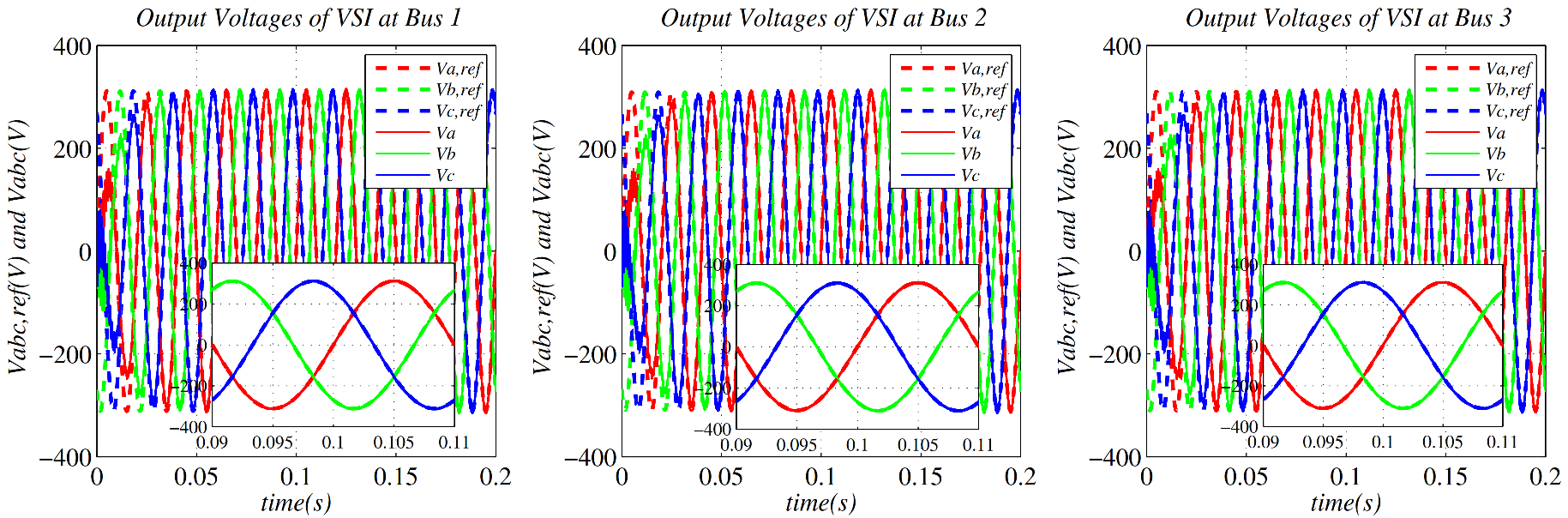
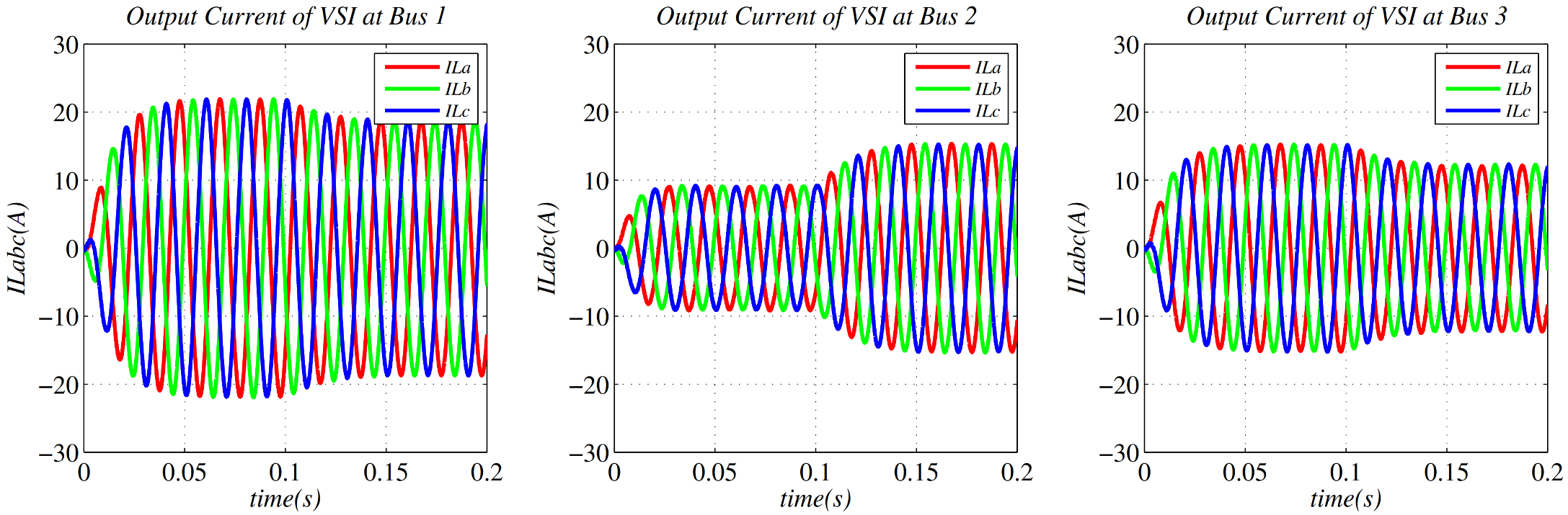
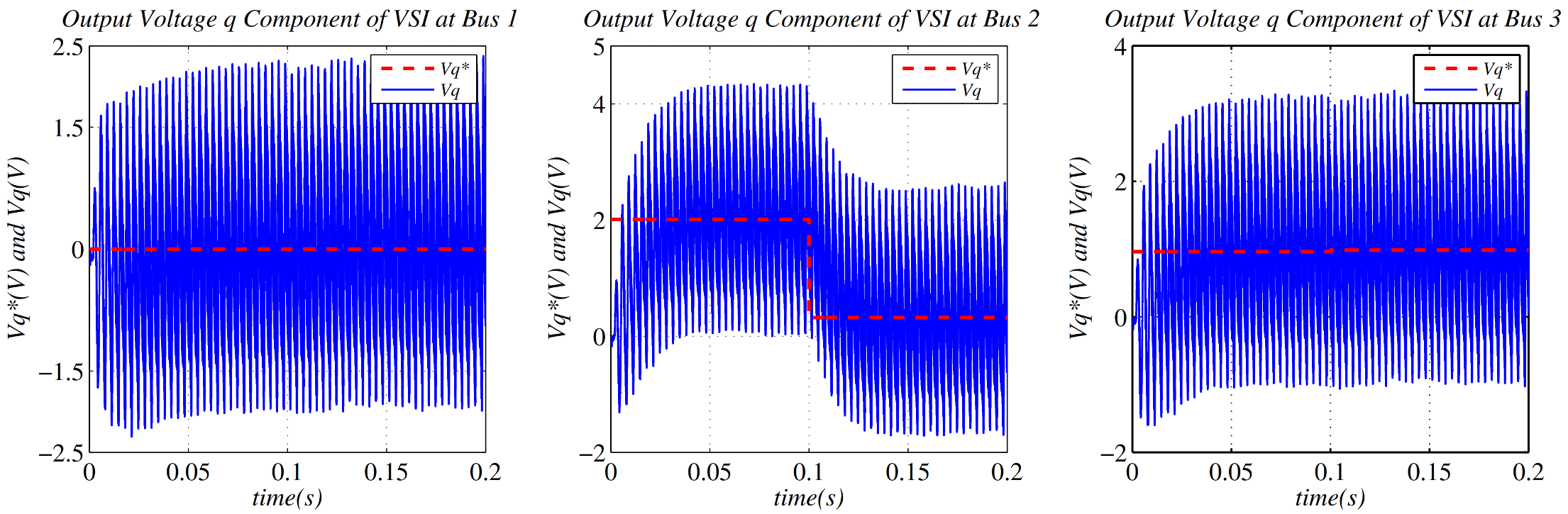
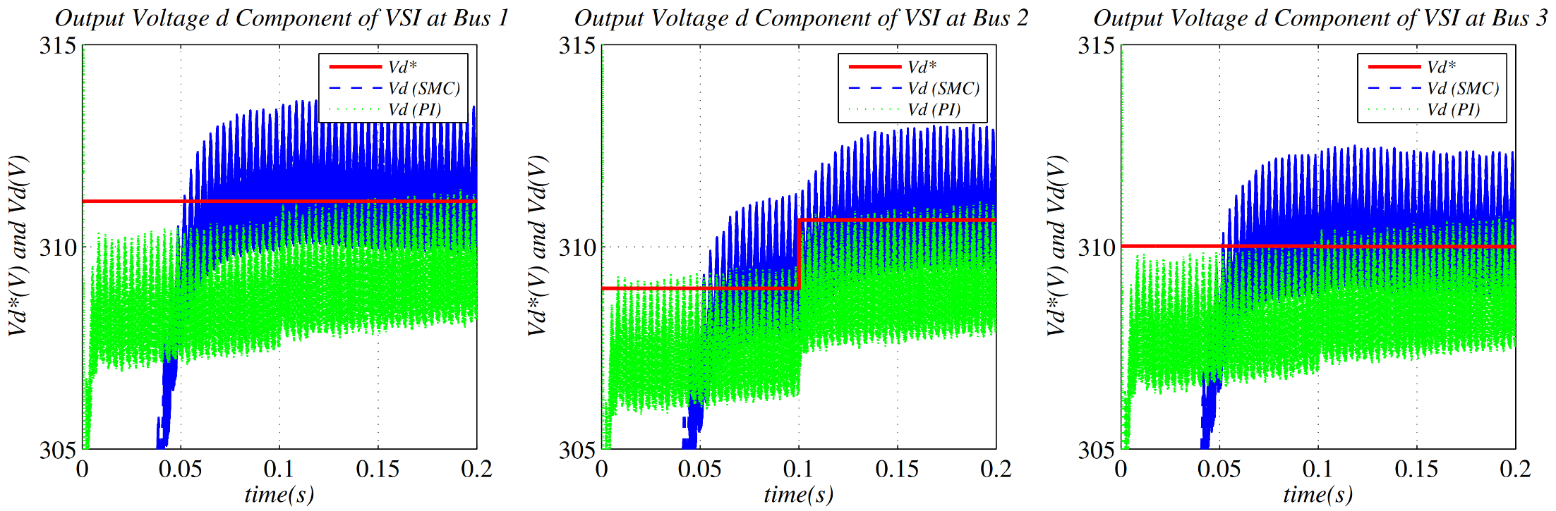
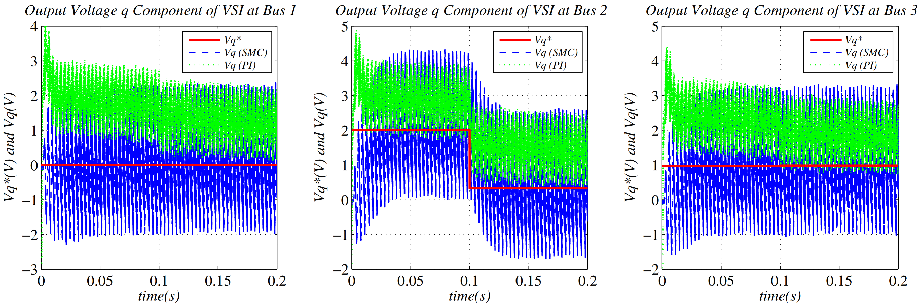
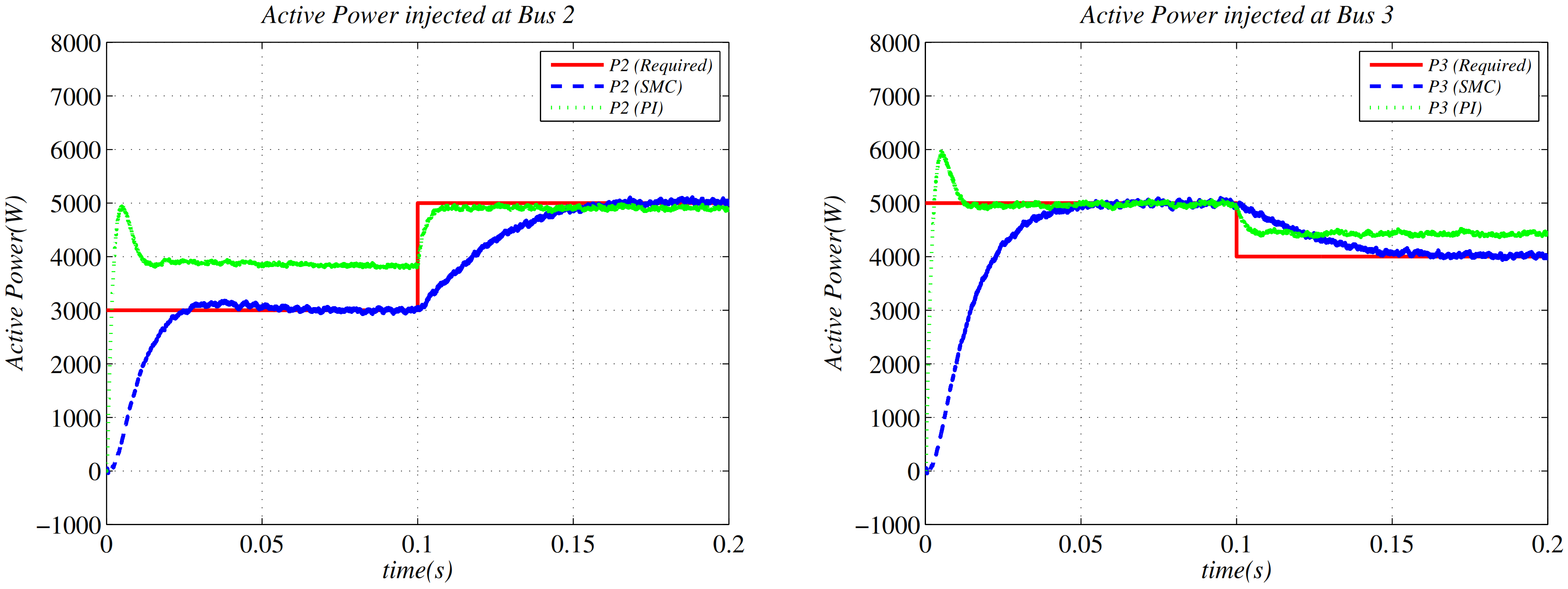
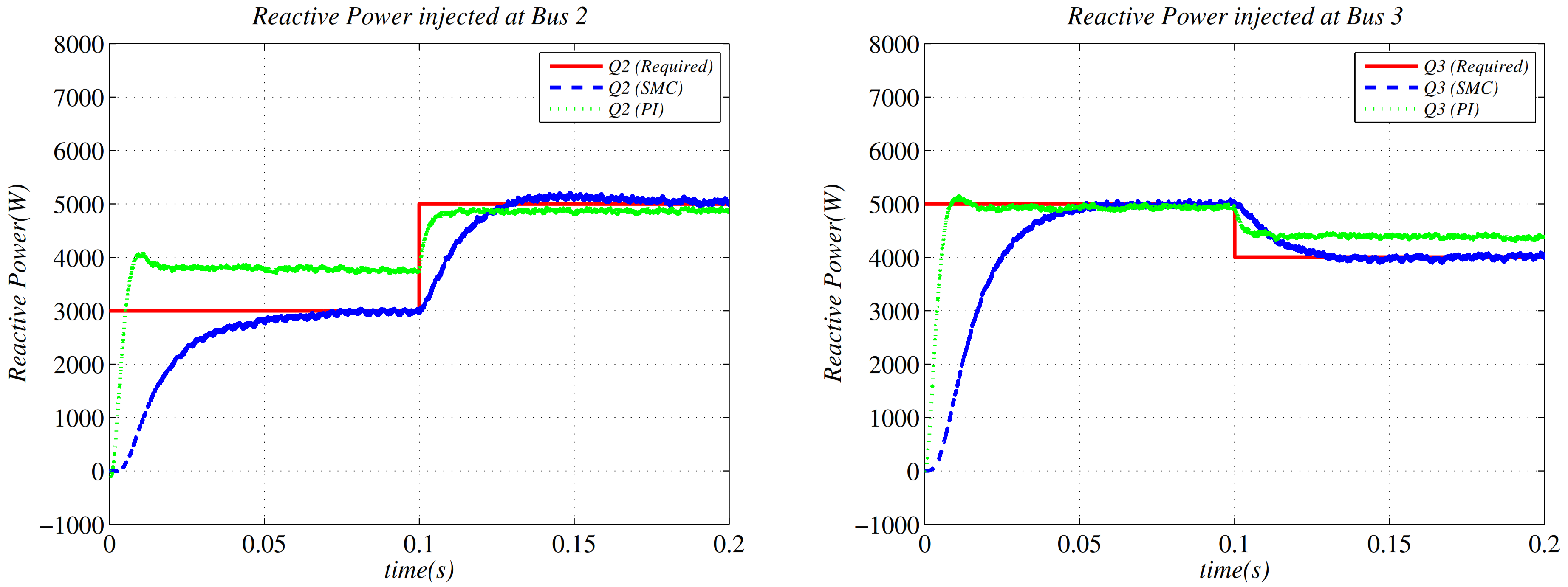
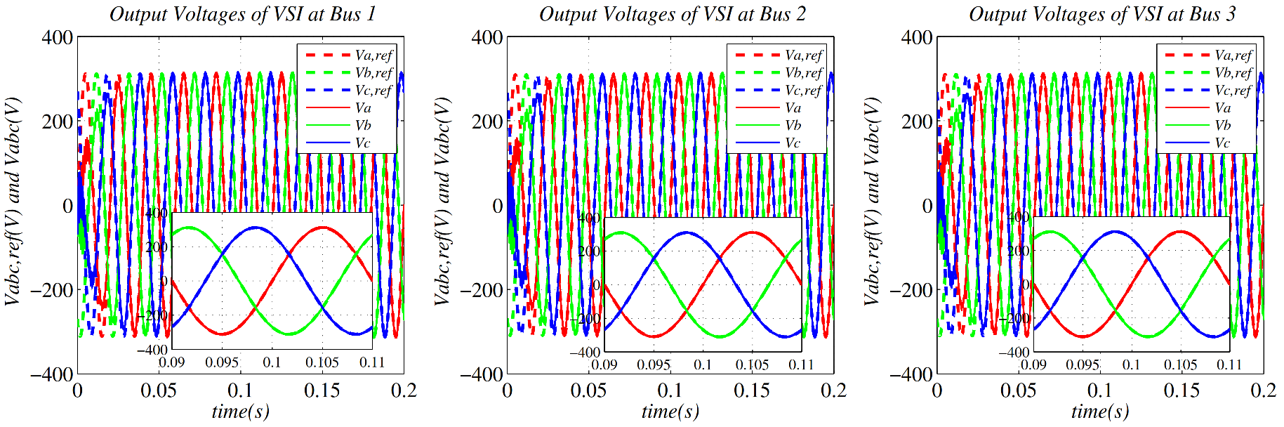
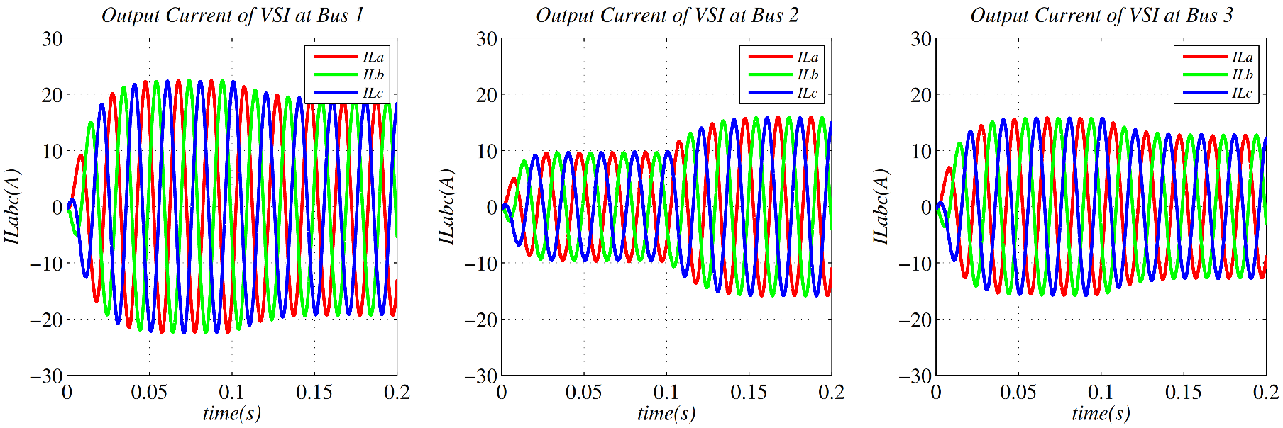
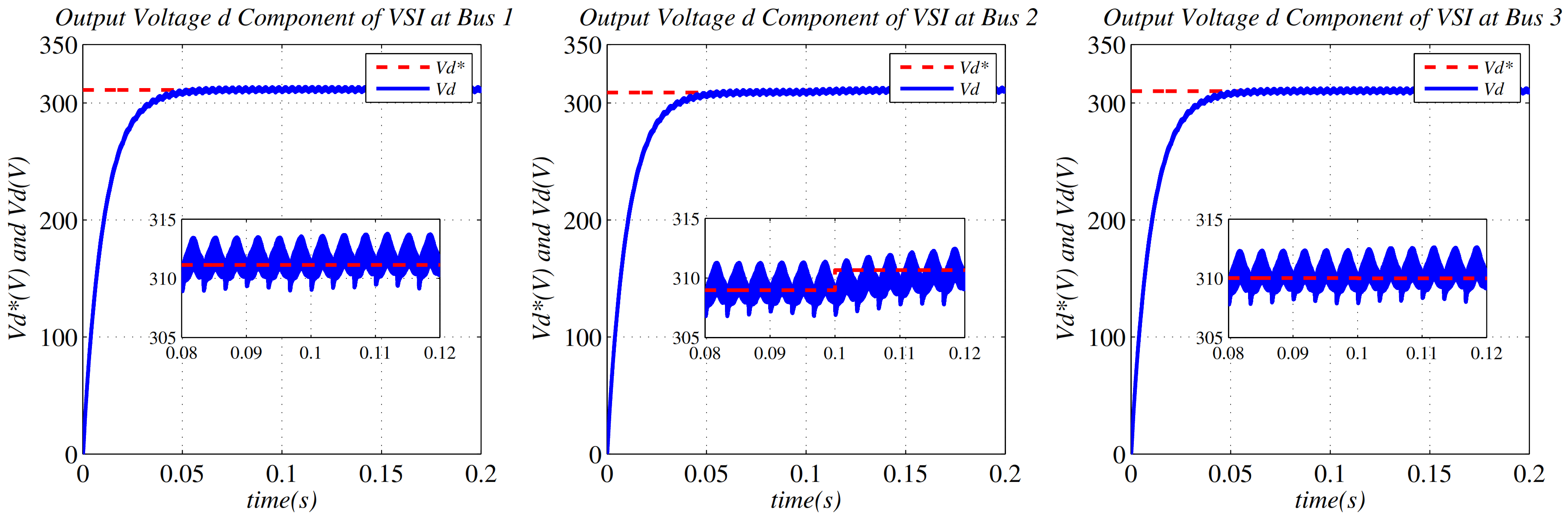
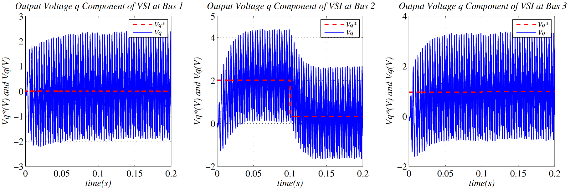
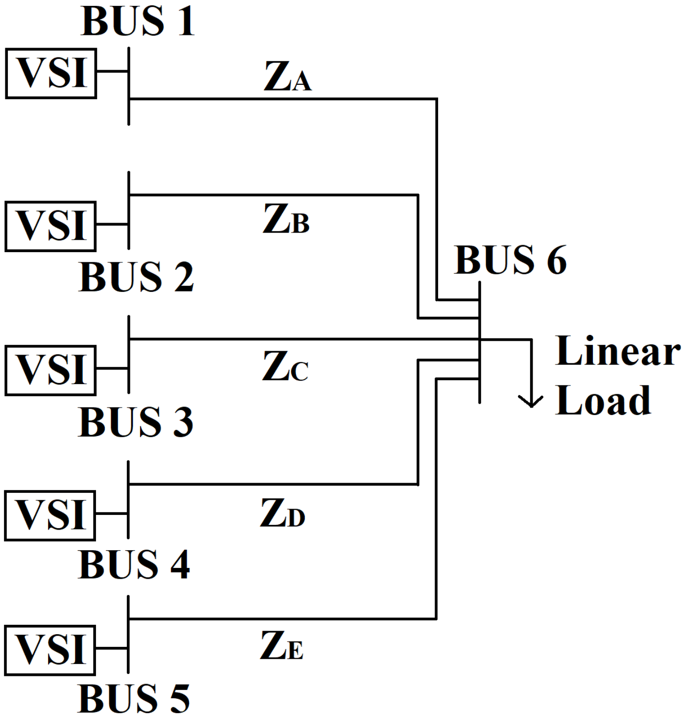
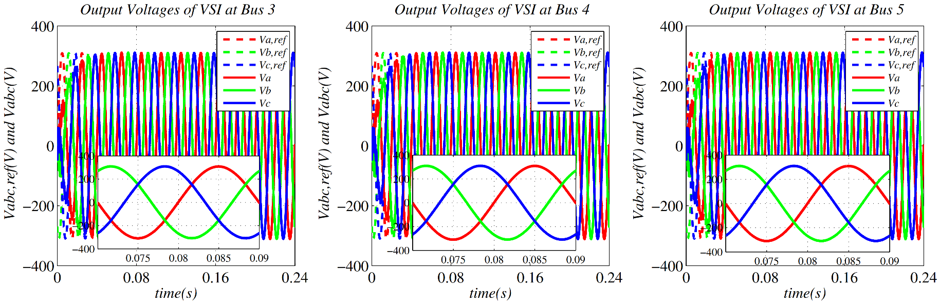
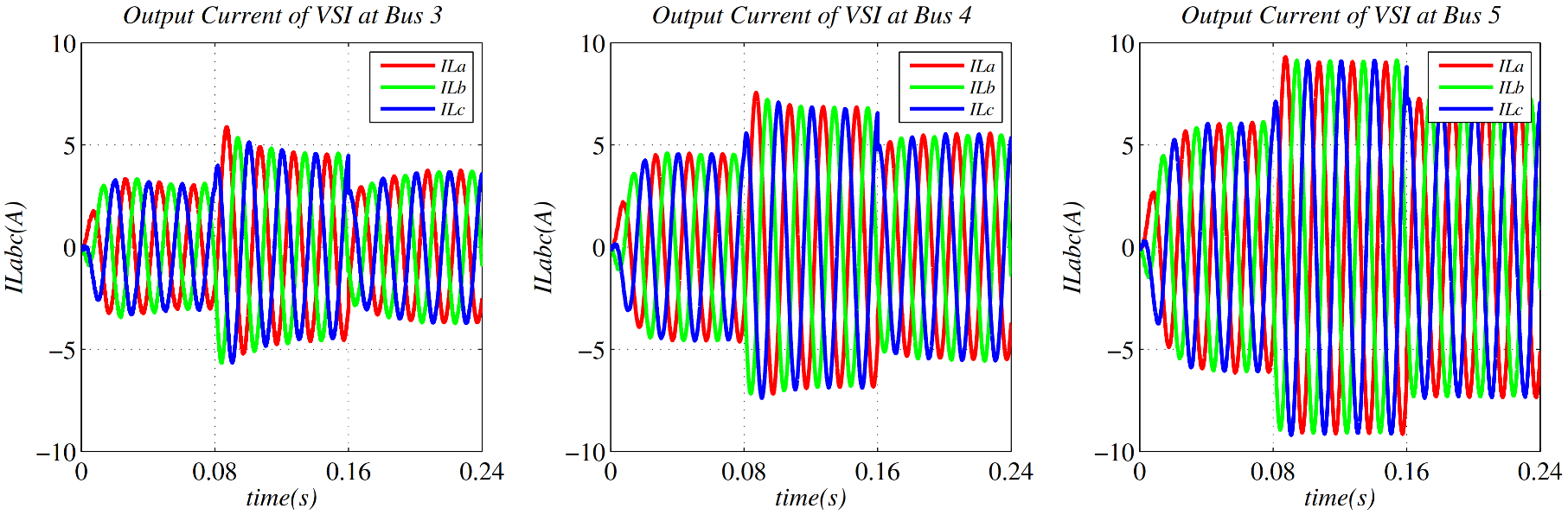
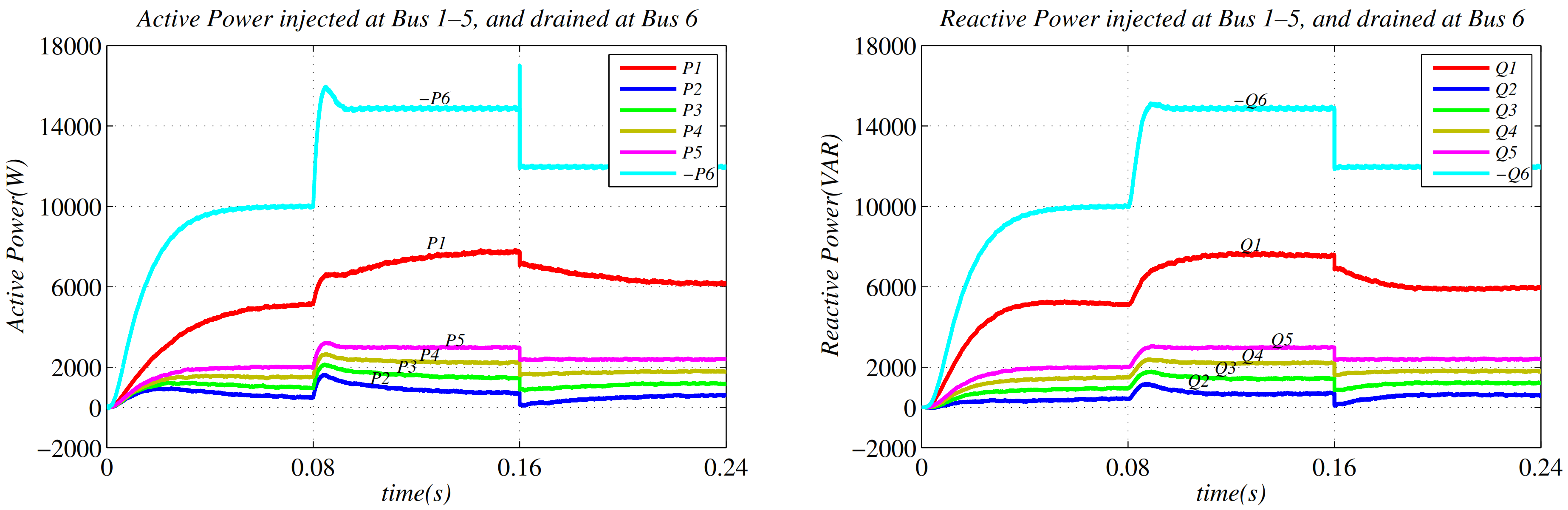
6. Simulation Results

In this section, the microgrid of four buses containing three inverters and a load bus are simulated by using the SimPowerSystems toolbox of Matlab/Simulink, as shown in Figure 3.

All VSIs used in the microgrid are identical and their electrical parameters are shown in

Table 1. Electrical parameters of the microgrid.

Electrical Parameters	Values
DC voltage source ($V_{dc}$)	1000 V
PWM carrier frequency	12.8 KHz
Nominal voltage of the system (phase-to-neutral)	$220V_{rms}$
Nominal frequency of the system $\left({\omega }_{\circ }\right)$	$100\pi$ rad/s
Resistance of the VSI output filter $\left(R_t\right)$	0.2 $\Omega$
Inductance of the VSI output filter $\left(L_t\right)$	1 mH
Capacitance of the VSI output filter $\left(C_t\right)$	20 $\mathsf{\mu }$F
Line resistance $\left(R_A\right)$	0.25 $\Omega$
Line inductance $\left(L_A\right)$	1.2 $\mathsf{\mu }$H
Line resistance $\left(R_B\right)$	0.27 $\Omega$
Line inductance $\left(L_B\right)$	1.3 $\mathsf{\mu }$H
Line resistance $\left(R_C\right)$	0.26 $\Omega$
Line inductance $\left(L_C\right)$	1.4 $\mathsf{\mu }$H

. The line impedance and admittance are calculated as

$$\begin{array}{cc}\hfill Z_A& =R_A+j{\omega }_{\circ }{L}_A,Y_A=\frac{1}{Z_A}\hfill \\ \hfill Z_B& =R_B+j{\omega }_{\circ }{L}_B,Y_B=\frac{1}{Z_B}\hfill \\ \hfill Z_C& =R_C+j{\omega }_{\circ }{L}_C,Y_C=\frac{1}{Z_C}\hfill \end{array}$$

(25)

The bus admittance matrix ${\mathbf{Y}}_{\mathbf{BUS}}$ for the microgrid shown in Figure 3 is as follows:

$${\mathbf{Y}}_{\mathbf{BUS}}=\left[\begin{array}{cccc}{Y}_A& 0& 0& -Y_A\\ 0& Y_B& 0& -Y_B\\ 0& 0& Y_C& -Y_C\\ -Y_A& -Y_B& -Y_C& Y_A+Y_B+Y_C\end{array}\right]$$

The active power, reactive power, and voltages for all buses of the microgrid operation are shown in

Table 2. Voltage and power details of the microgrid operation for $0\le t<0.1$ s.

Bus i	$|{\mathit{V}}_{\mathit{i}}|\left({\mathit{V}}_{\mathbf{rms}}\right)$	$\mathit{\angle }{\mathit{V}}_{\mathit{i}}\left(\mathbf{rad}\right)$	${\mathit{P}}_{\mathit{i}}\left(\mathit{W}\right)$	${\mathit{Q}}_{\mathit{i}}\left(\mathbf{VAR}\right)$
Bus 1	$\sqrt{3}\times 220$	0	$7K+\mathrm{losses}$	$7K+\mathrm{losses}$
Bus 2	$\sqrt{3}\times 218.4811$	$0.0065$	$3K$	$3K$
Bus 3	$\sqrt{3}\times 219.2180$	$0.0031$	$5K$	$5K$
Bus 4	$\sqrt{3}\times 217.2469$	$0.0122$	$-15K$	$-15K$

and

Table 3. Voltage and power details of the microgrid operation for $t\ge 0.1$ s.

Bus i	$|{\mathit{V}}_{\mathit{i}}|\left({\mathit{V}}_{\mathbf{rms}}\right)$	$\mathit{\angle }{\mathit{V}}_{\mathit{i}}\left(\mathbf{rad}\right)$	${\mathit{P}}_{\mathit{i}}\left(\mathit{W}\right)$	${\mathit{Q}}_{\mathit{i}}\left(\mathbf{VAR}\right)$
Bus 1	$\sqrt{3}\times 220$	0	$6K+\mathrm{losses}$	$6K+\mathrm{losses}$
Bus 2	$\sqrt{3}\times 219.6713$	$0.0010$	$5K$	$5K$
Bus 3	$\sqrt{3}\times 219.2077$	$0.0032$	$4K$	$4K$
Bus 4	$\sqrt{3}\times 217.6293$	$0.0104$	$-15K$	$-15K$

. Bus 1 is selected as the slack bus. Buses 2, 3, and 4 are PQ buses. PQ buses have defined active and reactive powers, and their voltages are calculated by Equation (23).

$|V_1|$ and $\angle V_1$ form the reference voltage signal for VSI at Bus 1 using Equations (24) and (3). Similarly, $|V_2|$ and $\angle V_2$ form the reference voltage signal for VSI at Bus 2, $|V_3|$ and $\angle V_3$ form the reference voltage signal for VSI at Bus 3. The controller that controls $V_d$ by generating the control signal $V_{td}$ is referred to as the “d controller”, and the controller that controls $V_q$ by generating the control signal $V_{tq}$ is referred to as the “q controller”. The controller parameters for both controllers are shown in

Table 4. Controller parameters of the VSI.

Controller Parameters	Values
a	200
b	$1.04$
c	$3.98\times {10}^{-4}$
$\beta$ for d controller	500
$\beta$ for q controller	250

, where a, b, and c values ($\mathbf{F}$ matrix) are the same for both controllers and are found by the pole placement method to achieve the desired settling time of “$0.04$ s”. The $\beta$ values for both controllers are found by inequalities (8) and (9) using the bounds given in

Table 5. Bounds on the system variables and parameters of the microgrid.

Bounds on the System Variables and Parameters
$-40\%$	$\le R_t\le$	$+40\%$
$-40\%$	$\le L_t\le$	$+40\%$
$-40\%$	$\le C_t\le$	$+40\%$
0	$\le x_{1d}\le$	350
0	$\le x_{2d}\le$	30
$-30$	$\le d_{1d}\le$	0
$-4\times {10}^3$	$\le d_{2d}\le$	$4\times {10}^3$
$-15\times {10}^3$	$\le {\dot{d}}_{1d}\le$	$6\times {10}^3$
$-100$	$\le x_{1q}\le$	150
$-12$	$\le x_{2q}\le$	10
$-10$	$\le d_{1q}\le$	10
$-9\times {10}^3$	$\le d_{2q}\le$	0
$-7\times {10}^3$	$\le {\dot{d}}_{1q}\le$	$7\times {10}^3$

.

The simulation results show that the error was ultimately bounded in finite time and the suggested power-sharing was also achieved. The output voltages of the inverters at Buses 1, 2, and 3 in the $abc$ reference frame are shown in Figure 4. It can be seen in Figure 4 that the output voltage of the inverters effectively tracks the reference signals. The current delivered by the inverters at Buses 1, 2, and 3 in the $abc$ reference frame are shown in Figure 5. The output voltage d components of the inverters at Buses 1, 2, and 3 are shown in Figure 6. In Figure 6, the performance of the "d controller" can be observed and its effective working can be seen. The output voltage reference tracking is effectively performed. The output voltage q components of the inverters at Buses 1, 2, and 3 are shown in Figure 7. From Figure 7, the performance of the "q controller" can be observed. The reference tracking is performed with the ultimately bounded error. This ultimately bounded error is due to the condition shown in Equation (15). Although the errors in the $dq$ reference frame are only ultimately bounded, the output voltages of the inverters in the $abc$ reference frame track their reference signals. The active power and reactive power injected at Buses 1, 2, and 3, and drained by the load at bus 4, are shown in Figure 8. The scheduled power-sharing shown in Table 2 and Table 3 can be observed in Figure 8. Thus, the required power-sharing was also achieved. It is due to the reference tracking of the inverter’s output voltages in the $abc$ reference frame.

The presented control design is also compared with PI controller-based cascaded voltage and current control of the microgrid [15], shown in Figure 9. The proportional and integral gains of the current controller are 10. The gains of the voltage controller are $0.1$. The results show that the performance of the control design presented in this paper gives better voltage regulation and power-sharing attainment. This PI control scheme has been widely used because of its ability to remove the steady-state error; eliminating the steady-state error while achieving the right transients is difficult with this PI control scheme. The output voltage d components of the inverters at Buses 1, 2, and 3 are shown in Figure 10. In this figure, a steady-state performance comparison is shown. It can be seen that the SMC design provides better reference tracking. The output voltage q components of the inverters at Buses 1, 2, and 3 are shown in Figure 11. The SMC design also provides better reference tracking of the output voltage’s q component. Due to better reference tracking of the output voltages d and q components by SMC, active and reactive power attainment are also better compared to PI control. The comparison of active power attainment by the SMC and PI controls of the VSIs at Buses 2 and 3 are shown in Figure 12. The reactive power comparison is shown in Figure 13. The better performance of SMC can be seen in all these comparison figures. Here, the SMC design is the output feedback, which used only the output voltage of the inverter. The PI control not only used the output voltage but also the $RLC$ filter’s input and output currents.

To check the performance of the presented controller design with the presence of the nonlinear load, a thyristor-based fully controlled bridge rectifier with a 1 k$\Omega$ resistance was attached on Buses 1, 2, and 3 as shown in Figure 14. The simulation results show that the error was ultimately bounded in the $dq$ reference frame and the scheduled power-sharing was achieved.

The output voltages of the inverters at Buses 1, 2, and 3 with the nonlinear load in the $abc$ reference frame are shown in Figure 15. With the presence of the nonlinear load, the inverter’s output voltage reference tracking in the $abc$ reference frame can be seen. The controller is effective as well in the presence of the nonlinear load. The current delivered by the inverters at Buses 1, 2, and 3 with the nonlinear load in the $abc$ reference frame are shown in Figure 16. The output voltage d components of the inverters at Buses 1, 2, and 3 with the nonlinear load are shown in Figure 17. The output voltage q components of the inverters at Buses 1, 2, and 3 with the nonlinear load are shown in Figure 18. In the $dq$ reference frame, the errors are still ultimately bounded with the nonlinear load. The active power and reactive power injected at Buses 1, 2, and 3 with the nonlinear load, and drained by the load at bus 4, are shown in Figure 19. Due to effective reference tracking of the inverter’s output voltage, the required power-sharing was also achieved.

To show the scalability of the proposed control scheme, a microgrid of six buses with five VSIs shown in Figure 20 was also simulated. In this simulation, the VSI parameters $Rt$, $Lt$, and $Ct$ were changed at $+40\%$ of their nominal values, to check the performance of the controller in the presence of parametric uncertainty. The load variation was also considered in this simulation. The line impedances $Z_A$, $Z_B$, and $Z_C$ were the same as in previous simulations. The line impedances $Z_D$ and $Z_E$ were considered the same as $Z_B$ and $Z_C$, respectively. VSI at Buses 2, 3, 4, and 5 shared $5\%$, $10\%$, $15\%$, and $20\%$ of the total load connected at bus 6, respectively. The remaining load was shared by the VSI connected at Bus 1.

The output voltages of the inverters connected at Buses 3, 4, and 5 in the $abc$ reference frame are shown in Figure 21. One could observe that the output voltages tracked their reference signals. The current delivered by the inverters at Buses 3, 4, and 5 in the $abc$ reference frame are shown in Figure 22. The active power and reactive power injected at Buses 1–5, and drained by the load at Bus 6, are shown in Figure 23. It is clearly demonstrated that the scheduled power-sharing was also achieved.

7. Conclusions

In this paper, the output voltage control problem of the VSI connected in the AC microgrid was considered. The sliding mode controller was designed in the $dq$ reference frame to asymptotically bring the error close to zero. The controller requires values of two states of the system. The first state is the inverter’s output voltage; for the second state, the VSI’s $RLC$ filter input and output currents are required. A high-gain observer was designed to estimate this second state of the system, which saves the requirement of two current sensors (only one voltage sensor is required). Stability analyses were shown for the controller and observer, clearly showing that the errors were converged and ultimately bounded. SMC provided robust stability for worst-case perturbations in the system variables and parameters. A high-gain observer also provided the state feedback performance with the output feedback controller, according to the separation principle. The active power and reactive power-sharing among multiple inverters connected in an AC microgrid were also considered. The required power-sharing was achieved by solving the power flow equations, which generated the reference signals of all inverters. The required power-sharing was also achieved, due to reference tracking of the inverter’s output voltages. The stability analysis and simulation results clearly show the effectiveness of the proposed control scheme, even in the presence of the nonlinear load and parametric uncertainty. A comparison of our design with the PI control was also presented, which showed the better performance of the presented control design.

References

1. Farrokhabadi, M.; Cañizares, C.A.; Simpson-Porco, J.W.; Nasr, E.; Fan, L.; Mendoza-Araya, P.A.; Tonkoski, R.; Tamrakar, U.; Hatziargyriou, N.; Lagos, D.; et al. Microgrid stability definitions, analysis, and examples. IEEE Trans. Power Syst. 2019, 35, 13–29. [Google Scholar] [CrossRef]
2. Olivares, D.E.; Mehrizi-Sani, A.; Etemadi, A.H.; Canizares, C.A.; Iravani, R.; Kazerani, M.; Hajimiragha, A.H.; Gomis-Bellmunt, O.; Saeedifard, M.; Palma-Behnke, R.; et al. Trends in the microgrid Control. IEEE Trans. Smart Grid 2014, 5, 1905–1919. [Google Scholar] [CrossRef]
3. Andishgar, M.H.; Gholipour, E.; Hooshm, R.A. An overview of control approaches of the inverter-based microgrids in islanding mode of operation. Renew. Sustain. Energy Rev. 2017, 80, 1043–1060. [Google Scholar] [CrossRef]
4. Zhou, Y.; Ho, C.N.M. A review on microgrid architectures and control methods. In Proceedings of the 8th International Power Electronics and Motion Control Conference (IPEMC-ECCE Asia), Hefei, China, 22–26 May 2016; pp. 3149–3156. [Google Scholar]
5. Guo, W.; Mu, L. Control principles of micro-source inverters used in the microgrid. Prot. Control Mod. Power Syst. 2016, 1, 1–7. [Google Scholar] [CrossRef]
6. Guerrero, J.M.; Chandorkar, M.; Lee, T.; Loh, P.C. Advanced Control Architectures for Intelligent Microgrids—Part I: Decentralized and Hierarchical Control. IEEE Trans. Ind. Electron. 2013, 60, 1254–1262. [Google Scholar] [CrossRef] [Green Version]
7. Rocabert, J.; Luna, A.; Blaabjerg, F.; Rodríguez, P. Control of Power Converters in AC Microgrids. IEEE Trans. Power Electron. 2012, 27, 4734–4749. [Google Scholar] [CrossRef]
8. Saad, N.H.; El-Sattar, A.A.; Mansour, A.E.-A.M. A novel control strategy for grid connected hybrid renewable energy systems using improved particle swarm optimization. Ain Shams Eng. J. 2018, 9, 2195–2214. [Google Scholar] [CrossRef]
9. Rezaei, N.; Mazidi, M.; Gholami, M.; Mohiti, M. A new stochastic gain adaptive energy management system for smart microgrids considering frequency responsive loads. Energy Rep. 2020, 6, 914–932. [Google Scholar] [CrossRef]
10. Parisio, A.; Rikos, E.; Glielmo, L.A. Model Predictive Control Approach to Microgrid Operation Optimization. IEEE Trans. Control Syst. Technol. 2014, 22, 1813–1827. [Google Scholar] [CrossRef]
11. Shrivastava, S.; Subudhi, B.; Das, S. Distributed voltage and frequency synchronisation control scheme for islanded inverter-based microgrid. IET Smart Grid 2018, 1, 48–56. [Google Scholar] [CrossRef]
12. Sadabadi, M.S.; Shafiee, Q.; Karimi, A. Plug-and-Play Voltage Stabilization in Inverter-Interfaced Microgrids via a Robust Control Strategy. IEEE Trans. Control Syst. Technol. 2016, 25, 781–791. [Google Scholar] [CrossRef] [Green Version]
13. Blaabjerg, F.; Teodorescu, R.; Liserre, M.; Timbus, A.V. Overview of Control and Grid Synchronization for Distributed Power Generation the systems. IEEE Trans. Ind. Electron. 2006, 53, 1398–1409. [Google Scholar] [CrossRef] [Green Version]
14. Chattopadhyay, S.; Mitra, M.; Sengupta, S. Clarke and Park Transform. In Electric Power Quality. Power Systems; Springer: Dordrecht, The Netherlands, 2011. [Google Scholar] [CrossRef]
15. Liu, R.; Wang, S.; Liu, G.; Wen, S.; Zhang, J.; Ma, Y. An Improved Virtual Inertia Control Strategy for Low Voltage AC Microgrids with Hybrid Energy Storage Systems. Energies 2022, 15, 442. [Google Scholar] [CrossRef]
16. He, J.; Li, Y.W. Generalized Closed-Loop Control Schemes with Embedded Virtual Impedances for Voltage Source Converters with LC or LCL Filters. IEEE Trans. Power Electron. 2012, 27, 1850–1861. [Google Scholar] [CrossRef]
17. Ebrahim, M.A.; Fattah, R.M.A.; Saied, E.M.M.; Maksoud, S.M.A.; Khashab, H.E. Real-time implementation of self-adaptive salp swarm optimization based microgrid droop control. IEEE Access 2020, 8, 185738–185751. [Google Scholar] [CrossRef]
18. Ebrahim, M.A.; Ayoub, B.A.A.; Nashed, M.N.F.; Osman, F.A.M. A Novel Hybrid-HHOPSO Algorithm Based Optimal Compensators of Four-Layer Cascaded Control for a New Structurally Modified AC Microgrid. IEEE Access 2020, 9, 4008–4037. [Google Scholar] [CrossRef]
19. Jiang, X.-Y.; He, C.; Jermsittiparsert, K. Online optimal stationary reference frame controller for inverter interfaced distributed generation in a microgrid system. Energy Rep. 2019, 6, 134–145. [Google Scholar] [CrossRef]
20. Gao, T.; Lin, Y.; Chen, D.; Xiao, L. A novel active damping control based on grid-side current feedback for LCL-filter active power filter. Energy Rep. 2020, 6 (Suppl. 9), 1318–1324. [Google Scholar] [CrossRef]
21. Agrawal, S.; Tyagi, B.; Kumar, V.; Sharma, P. 3ph qZSI Controller Design using PI for DC side and PR for AC side Controller including Droop Characteristic in standalone mode. In Proceedings of the IEEE International Conference on Power Electronics, Smart Grid, and Renewable Energy (PESGRE), Trivandrum, India, 2–5 January 2022; pp. 1–6. [Google Scholar] [CrossRef]
22. Mohiuddin, S.M.; Qi, J. Optimal Distributed Control of AC Microgrids With Coordinated Voltage Regulation and Reactive Power Sharing. IEEE Trans. Smart Grid 2022, 13, 1789–1800. [Google Scholar] [CrossRef]
23. Perez-Ibacache, R.; Castro, R.S.; Pimentel, G.A.; Bizzo, B.S. Dynamic Output-Feedback Decentralized Control Synthesis for Integration of Distributed Energy Resources in AC Microgrids. IEEE Trans. Smart Grid 2021, 13, 1225–1237. [Google Scholar] [CrossRef]
24. Batmani, Y.; Khayat, Y.; Najafi, S.; Guerrero, J.M. Optimal Integrated Inner Controller Design in AC Microgrids. IEEE Trans. Power Electron. 2022, 37, 10372–10383. [Google Scholar] [CrossRef]
25. Hu, C.; Liu, C.; Luo, S.; Yan, H. Joint Control Strategy of the microgrid Inverter Based on Optimal Control and Residual Dynamic Compensation. J. Phys. 2022, 2215, 012003. [Google Scholar] [CrossRef]
26. Yaramasu, V.; Rivera, M.; Narimani, M.; Wu, B.; Rodriguez, J. Model Predictive Approach for a Simple and Effective Load Voltage Control of Four-Leg Inverter with an Output LC Filter. IEEE Trans. Ind. Electron. 2014, 61, 5259–5270. [Google Scholar] [CrossRef]
27. Ma, D.; Cao, X.; Sun, C.; Wang, R.; Sun, Q.; Xie, X.; Peng, W. Dual-Predictive Control With Adaptive Error Correction Strategy for AC Microgrids. IEEE Trans. Power Deliv. 2021, 37, 1930–1940. [Google Scholar] [CrossRef]
28. Shan, Y.; Pan, A.; Liu, H. A Switching Event-Triggered Resilient Control Scheme for Primary and Secondary Levels in AC Microgrids. ISA Trans. 2022, in press. [Google Scholar] [CrossRef]
29. Konneh, K.V.; Adewuyi, O.B.; Lotfy, M.E.; Sun, Y.; Senjyu, T. Application Strategies of the model Predictive Control for the Design and Operations of Renewable Energy-Based Microgrid: A Survey. Electronics 2022, 11, 554. [Google Scholar] [CrossRef]
30. Baghaee, H.R.; Mirsalim, M.; Gharehpetian, G.B.; Talebi, H.A. A Decentralized Robust Mixed H2/H Voltage Control Scheme to Improve Small/Large-Signal Stability and FRT Capability of Islanded Multi-DER Microgrid Considering Load Disturbances. IEEE Syst. J. 2017, 12, 2610–2621. [Google Scholar] [CrossRef]
31. Babazadeh, M.; Karimi, H. A Robust Two-Degree-of-Freedom Control Strategy for an Islanded Microgrid. IEEE Trans. Power Deliv. 2013, 28, 1339–1347. [Google Scholar] [CrossRef]
32. Fathi, A.; Shafiee, Q.; Bevrani, H. Robust Frequency Control of the microgrids Using an Extended Virtual Synchronous Generator. IEEE Trans. Power Syst. 2018, 33, 6289–6297. [Google Scholar] [CrossRef]
33. Derakhshan, S.; Shafiee-Rad, M.; Shafiee, Q.; Jahed-Motlagh, M.R. Decentralized Robust Voltage Control of Islanded AC Microgrids: An LMI-Based H Approach. In Proceedings of the 11th Power Electronics, Drive Systems, and Technologies Conference (PEDSTC), Tehran, Iran, 4–6 February 2020; pp. 1–6. [Google Scholar] [CrossRef]
34. Shafiee-Rad, M.; Shafiee, Q.; Motlagh, M.-R.J. Decentralized Scalable Robust Voltage Control for Islanded AC Microgrids with General Topology. In Proceedings of the 11th Power Electronics, Drive Systems, and Technologies Conference (PEDSTC), Tehran, Iran, 4–6 February 2020; pp. 1–6. [Google Scholar] [CrossRef]
35. Shi, M.; Chen, X.; Shahidehpour, M.; Zhou, Q.; Wen, J. Observer-Based Resilient Integrated Distributed Control Against Cyberattacks on Sensors and Actuators in Islanded AC Microgrids. IEEE Trans. Smart Grid 2021, 12, 1953–1963. [Google Scholar] [CrossRef]
36. Jouda, M.S.; Kahraman, N. Improved Optimal Control of Transient Power Sharing in the microgrid Using H-Infinity Controller with Artificial Bee Colony Algorithm. Energies 2022, 15, 1043. [Google Scholar] [CrossRef]
37. Gholami, S.; Saha, S.; Aldeen, M. Robust multiobjective control method for power sharing among distributed energy resources in islanded microgrids with unbalanced and nonlinear loads. Int. J. Electr. Power Energy Syst. 2018, 94, 321–338. [Google Scholar] [CrossRef]
38. Raeispour, M.; Atrianfar, H.; Baghaee, H.R.; Gharehpetian, G.B. Robust Sliding Mode and Mixed H2/H Output Feedback Primary Control of AC Microgrids. IEEE Syst. J. 2020, 15, 2420–2431. [Google Scholar] [CrossRef]
39. Hu, W.; Shen, Y.; Yang, Z.; Min, H. Mixed H2/H Optimal Voltage Control Design for Smart Transformer Low-Voltage Inverter. Energies 2022, 15, 365. [Google Scholar] [CrossRef]
40. Hua, H.; Qin, Y.; He, Z.; Li, L.; Cao, J. Energy sharing and frequency regulation in energy network via mixed H2/H control with Markovian jump. CSEE J. Power Energy Syst. 2020, 7, 1302–1311. [Google Scholar]
41. Azizi, S.M. Robust Controller Synthesis and Analysis in Inverter-Dominant Droop-Controlled Islanded Microgrids. IEEE/CAA J. Autom. Sin. 2021, 8, 1401–1415. [Google Scholar] [CrossRef]
42. Chen, Z.; Luo, A.; Wang, H.; Chen, Y.; Li, M.; Huang, Y. Adaptive sliding-mode voltage control for inverter operating in islanded mode in the microgrid. Int. J. Electr. Power Energy Syst. 2015, 66, 133–143. [Google Scholar] [CrossRef]
43. Kalla, U.K.; Singh, B.; Murthy, S.S.; Jain, C.; Kant, K. Adaptive Sliding Mode Control of Standalone Single-Phase Microgrid Using Hydro, Wind, and Solar PV Array-Based Generation. IEEE Trans. Smart Grid 2017, 9, 6806–6814. [Google Scholar] [CrossRef]
44. Xu, D.; Dai, Y.; Yang, C.; Yan, X. Adaptive fuzzy sliding mode command-filtered backstepping control for islanded PV microgrid with energy storage system. J. Frankl. Inst. 2019, 356, 1880–1898. [Google Scholar] [CrossRef]
45. Hu, J.; Sun, Q.; Wang, R.; Wang, B.; Zhai, M.; Zhang, H. Privacy-Preserving Sliding Mode Control for Voltage Restoration of AC Microgrids Based on Output Mask Approach. IEEE Trans. Ind. Inf. 2022, 18, 6818–6827. [Google Scholar] [CrossRef]
46. Krishnan, U.B.; Mija, S.J.; Cheriyan, E.P. Improved small signal stability of the microgrid—A droop control scheme with SMC. Electr. Eng. 2022, 1–19. [Google Scholar] [CrossRef]
47. Yang, C.; Hua, T.; Dai, Y.; Liu, G.; Huang, X.; Zhang, D. Disturbance-Observer-Based Adaptive Fuzzy Control for Islanded Distributed Energy Resource Systems. Math. Probl. Eng. 2022, 2022, 1527705. [Google Scholar] [CrossRef]
48. Al Sumarmad, K.A.; Sulaiman, N.; Wahab, N.I.A.; Hizam, H. Energy Management and Voltage Control in the microgrids Using Artificial Neural Networks, PID, and Fuzzy Logic Controllers. Energies 2022, 15, 303. [Google Scholar] [CrossRef]
49. Nasir, M.; Bansal, R.; Elnady, A. A Review of Various Neural Network Algorithms for Operation of AC Microgrids. In Proceedings of the 2022 Advances in Science and Engineering Technology International Conferences (ASET), Dubai, United Arab Emirates, 21–24 February 2022; pp. 1–7. [Google Scholar] [CrossRef]
50. Trivedi, R.; Khadem, S. Implementation of artificial intelligence techniques in the microgrid control environment: Current progress and future scopes. Energy 2022, 8, 100147. [Google Scholar] [CrossRef]
51. Etemadi, A.H.; Davison, E.J.; Iravani, R. A Generalized Decentralized Robust Control of Islanded Microgrids. IEEE Trans. Power Syst. 2014, 29, 3102–3113. [Google Scholar] [CrossRef]
52. Molzahn, D.K.; Dorfler, F.; Sandberg, H.; Low, S.H.; Chakrabarti, S.; Baldick, R.; Lavaei, J. A Survey of Distributed Optimization and Control Algorithms for Electric Power Systems. IEEE Trans. Smart Grid 2017, 8, 2941–2962. [Google Scholar] [CrossRef]
53. Atassi, A.; Khalil, H. A separation principle for the stabilization of a class of the nonlinear systems. IEEE Trans. Autom. Control 1999, 44, 1672–1687. [Google Scholar] [CrossRef]
54. Khalil, H.K. Nonlinear Systems, 3rd ed.; Prentice Hall: Upper Saddle River, NJ, USA, 2002. [Google Scholar]
55. Khalil, H.K. High-gain observers in nonlinear feedback control. In Proceedings of the International Conference on Control, Automation and Systems, Seoul, Korea, 14–17 October 2008; pp. xlvii–lvii. [Google Scholar] [CrossRef]
56. Kothari, D.P.; Nagrath, I.J. Modern Power System Analysis; Tata McGraw-Hill: New York, NY, USA, 2003. [Google Scholar]
Figure 1. Voltage source inverter (VSI) with the output filter.
Energies 15 05586 g001
Figure 2. SMC with an HGO-based control scheme applied for the VSI voltage control.
Energies 15 05586 g002
Figure 3. Microgrid of four buses.
Energies 15 05586 g003
Figure 4. Output voltages of the VSI at Buses 1, 2, and 3 in the a b c reference frame.
Energies 15 05586 g004
Figure 5. Output current of the VSI at Buses 1, 2, and 3 in the a b c reference frame.
Energies 15 05586 g005
Figure 6. Output voltage d component of the VSI at Buses 1, 2, and 3.
Energies 15 05586 g006
Figure 7. Output voltage q component of the VSI at Buses 1, 2, and 3.
Energies 15 05586 g007
Figure 8. Active power and reactive power injected at Buses 1, 2, and 3, and drained at Bus 4.
Energies 15 05586 g008
Figure 9. PI-based control scheme applied to the VSI voltage control.
Energies 15 05586 g009
Figure 10. Output voltage d components of the VSI at Buses 1, 2, and 3 (comparison of the SMC and PI controls).
Energies 15 05586 g010
Figure 11. Output voltage q components of the VSI at Buses 1, 2, and 3 (comparison of the SMC and PI controls).
Energies 15 05586 g011
Figure 12. Active power injected at Buses 2 and 3 (comparison of the SMC and PI controls).
Energies 15 05586 g012
Figure 13. Reactive power injected at Buses 2 and 3 (comparison of the SMC and PI controls).
Energies 15 05586 g013
Figure 14. Microgrid of four buses with nonlinear loads.
Energies 15 05586 g014
Figure 15. Output voltages of the VSI at Buses 1, 2, and 3 with the nonlinear load in the a b c reference frame.
Energies 15 05586 g015
Figure 16. Output current of the VSI at Buses 1, 2, and 3 with the nonlinear load in the a b c reference frame.
Energies 15 05586 g016
Figure 17. Output voltage d component of the VSI at Buses 1, 2, and 3 with the nonlinear load.
Energies 15 05586 g017
Figure 18. Output voltage q component of the VSI at Buses 1, 2, and 3 with the nonlinear load.
Energies 15 05586 g018
Figure 19. Active power and reactive power injected at Buses 1, 2, and 3 with the nonlinear load, and drained at Bus 4.
Energies 15 05586 g019
Figure 20. Microgrid of six buses.
Energies 15 05586 g020
Figure 21. Output voltages of the VSI at Buses 3, 4, and 5 in the a b c reference frame (six-bus microgrid).
Energies 15 05586 g021
Figure 22. Output currents of the VSI at Buses 3, 4, and 5 in the a b c reference frame (six-bus microgrid).
Energies 15 05586 g022
Figure 23. Active power and reactive power injected at Buses 1–5, and drained at Bus 6 (six-bus microgrid).
Energies 15 05586 g023