A Data-Driven Reduced-Order Model for Estimating the Stimulated Reservoir Volume (SRV)

Abstract

The main goal of hydraulic fracturing stimulation in unconventional and tight reservoirs is to maximize hydrocarbon production by creating an efficient stimulated reservoir volume (SRV) around the horizontal wells. To zreach this goal, a physics-based model is typically used to design and optimize the hydraulic fracturing process before executing the job. However, two critical issues make this approach insufficient for achieving the mentioned goal. First, the physics-based models are based on several simplified assumptions and do not correctly represent the physics of unconventional reservoirs; hence, they often fail to match the observed SRVs in the field. Second, the success of the executed stimulation job is evaluated after it is completed in the field, leaving no room to modify some parameters such as proppant concentration in the middle of the job. To this end, this paper proposes data-driven and global sensitivity approaches to address these two issues. It introduces a novel workflow for estimating SRV in near real-time using some hydraulic fracturing parameters that can be inferred before or during the stimulation process. It also utilizes a robust global sensitivity framework known as the Sobol Method to rank the input parameters and create a reduced-order (mathematically simple) model for near real-time estimation of SRV (referred to as DSRV). The proposed framework in this paper has two main advantages and novelties. First, it is based on a pure data-based approach, with no simplified assumptions due to the use of a simulator for generating the training and test dataset, which is often the case in similar studies. Second, it treats SRV generation as a rock mechanics problem (rather than a reservoir engineering problem with fixed fracture lengths), accounting for changes in hydraulic fracture topology and SRV changes with time. A dataset from the Marcellus Shale Energy and Environment Laboratory (MSEEL) project is used. The model’s input parameters include stimulation variables of 58 stages of two wells. These parameters are stage number, step, pump rate and duration, proppant concentration and mass, and treating pressure. The model output consists of the corresponding microseismic (MS) cloud size at each step (i.e., time window) during the job. Based on the model, guidelines are provided to help operators design more efficient fracturing jobs for maximum recovery and to monitor the effectiveness of the hydraulic fracturing process. A few future improvements to this approach are also provided.

1. Introduction

Hydraulic fracturing stimulation is an integrated part of unconventional and tight reservoir development. Its primary purpose is to maximize hydrocarbon recovery by creating an efficient stimulated reservoir volume (SRV) around horizontal wells. A conventional approach for designing hydraulic fracturing parameters, such as proppant concentration, fluid type, and rate, is to run several simulated reservoir models with different parameters. This approach has two shortcomings: the simplified assumptions of the simulator and computational cost. The physics-based models used for building simulated reservoir models do not often represent the physics of fluid flow in unconventional and tight reservoirs. They also fail to account for the high uncertainty involved in reservoir properties in these reservoirs. Moreover, the high computational cost is a severe bottleneck for the coupled flow-geomechanical simulation of tight and unconventional reservoirs. Ref. [1] compared the run time of a high-fidelity physics-based model with the pre-processing and runtime of three data-driven models. They showed that the run time of a high-fidelity numerical model can reach up to ~3000 times compared to the data-based model. Although recursive model updating could be utilized to reduce the computation time of dynamic models, a more efficient approach for designing and controlling the hydraulic fracturing process is desired. This study proposes two frameworks, namely, pure data-driven and reduced-order SRV modeling, to address the issues mentioned in using high-fidelity numerical models for solving hydraulic fracturing problems. Our approach differs from most previous studies by accounting for dynamic changes in the fractured zone topology, allowing for different fractured volumes along the length of the horizontal well. The other difference between this approach and similar works is that it is purely based on field-recorded data and not on synthetic data (typical) generated by numerical models.

In the last decade, a rich body of literature has been produced for solving production-related and hydraulic fracturing problems of unconventional reservoirs using data-based models. Refs. [2,3] utilized data-based approaches to optimize the design of the hydraulic fracturing process in unconventional reservoirs. They developed models using random forest and artificial neural networks (ANN) and used parameters such as TVD and proppant volume to estimate the first-year production from unconventional fractured wells. Ref. [4] built ANN models to predict the first-year production from geologic and completion input parameters such as porosity, depth, and water saturation in the Mid Bakken formation. Ref. [5] used a long short-term memory (LSTM) neural network to predict gas production from shale formations. Ref. [6] utilized machine learning and reduced-order models for forecasting gas production from unconventional reservoirs. Ref. [7] studied the HF–NF interactions and their significance for SRV development. They also used machine learning to rank the importance of parameters involved in HF–NF interactions. Ref. [8] applied a machine learning approach for modeling SRV, fracture network characterization, and well interference. Ref. [9] presented a state-of-the-art review on hydraulic fracture modeling using machine learning (ML)/artificial intelligence (AI) algorithms, focusing on design, interpretation, real-time prediction, and re-frac candidate selection. Other examples can be found in [10,11], where the effect of several input parameters on SRV was examined using fully synthetic data from a simulator. In [11], the well spacing was examined to avoid frac-hit while drilling more wells in the field.

There are two general approaches for solving and optimizing hydraulic fracturing problems: the pure fracturing approach and the reservoir/production approach. The pure fracturing approach typically involves using fracturing parameters such as surface pressure and proppant concentration and predicting production directly. However, most reservoir/production approaches focused on production prediction, and less attention was given to predicting SRV’s dynamic growth (size and direction). They typically used SRV as an input to their models for predicting the production in the future or as a tool to estimate the total production from a well. In addition, the input data set for the training of both approaches is mainly generated using a high-fidelity numerical simulator (c.f., [1]). Another shortcoming of this approach is that most of the fractures along the length of the horizontal well are assumed to have the same length. This assumption contradicts the field evidence that only 70–80% of the stages contribute to production and that the majority of production comes from only 20–30% of the clusters [12,13]. In addition, due to the perturbed stress regime in multistage hydraulic fracking of horizontal stress (known as stress shadow), hydraulic fractures in a horizontal well will have different topologies [14]. The low efficiency is due to high uncertainty in unconventional reservoirs and an inefficient hydraulic fracturing design. Therefore, there is a gap in the literature for a data-driven model that can account for dynamic changes in the SRV along the length of the horizontal well.

Sensitivity analysis (SA) is a common approach used for quantifying the importance of the models’ input parameters to the variance of the output parameter(s). Generally, there are two types of sensitivity analysis: global sensitivity analysis (GSA) and local sensitivity analysis (LSA) [15,16]. The difference between these two approaches is that the uncertainty of the output parameter from simultaneous changes in all input parameters is investigated in GSA, while in LSA, the uncertainty of the individual parameters is studied. Refs. [17,18] developed a GSA method for calculating the input variable(s) influences on the output of a complicated mathematical model. The advantage of this method over other GSA techniques is that it can be applied to highly nonlinear functions and even in situations where the governing function is not known explicitly. The technique can also be used to create reduced-order models (ROM) for the original function. ROM is a simplified model, typically polynomial, built using a complex base model and can represent it with a controlled error. This study used the Sobol GSA technique to build a ROM for estimating SRV in near real-time. Ref. [19] used the Sobol method to rank the parameters affecting the pore pressure and stresses around hydraulic fractures. They also developed a ROM for calculating pressure and stresses around hydraulic fractures. Ref. [20] developed a fully coupled hydro-mechanical ROM to simulate fractured media. Ref. [21] presented a ROM for the propagation of multiple radial hydraulic fractures. Ref. [22] calculated the pressure drop due to stress shadow along the fractures in a horizontal well using a data-based ROM. Ref. [23] introduce sparse proper orthogonal decomposition (SPOD)–Galerkin methodology for deriving ROMs for propagating fractures. In all the studies mentioned here, the ROM is typically built for analyzing the primary hydraulic(s) behavior, and less attention is given to estimating the SRV containing the induced and activated microfractures critical in production from unconventional and tight reservoirs.

This paper uses a similar workflow to [24] to fill a gap in the literature and introduce a framework for estimating the SRV in near real-time. Two central parts of this research are a predictive (data-based) model and a ROM. In the first part, several ML algorithms are developed and used to predict SRV in small time steps. A time-lapse prediction of SRV is called dynamic SRV (DSRV). The hydraulic fracturing data of wells MIP-3H and MIP-5H from the Marcellus Shale Energy and Environment Laboratory (MSEEL) project are used to predict a volume enclosing most microseismic events and at different steps from the beginning of the job. The second part developed an efficient near-real-time ROM for the created data-driven models. The ROM is built based on previous studies (e.g., [24]) and can easily be used to improve the effectiveness of the well stimulation process. It can also be used to estimate the SRV (quantity of interest (QI) in this study) in near-real-time (i.e., seconds or minutes) and at any location and time along the lateral of the horizontal well. Temporal and spatial estimations of the mentioned QIs are essential for visualizing the fluid flow and depletion.

The paper is organized as follows. Section 2 briefly describes the workflow and details of the methodologies used in this paper. The specifics of data-based models, including the pre-processing, input and output data generation, and created models hyperparameters, are summarized in Section 2.1. In Section 2.2, the mathematical background of the Sobol global sensitivity analysis is presented. A workflow using the Sobol method for complex (not known explicitly) functions is also presented. Then, the results of the generated ML models are discussed in Section 3. Section 3.1 starts with the performance evaluation of the models and then presents a GSA of the created models for ranking the importance of the input parameters in Section 3.2. Later, a ROM for estimating SRV in near-real-time is presented in Section 3.3. In Section 3.4, suggestions for further improvements of the models are given. Lastly, a summary of the research and conclusions are drawn in Section 4.

2. Methodologies and Mathematical Formulation

During a typical hydraulic fracturing job, different types of information are recorded. From this information, design-related parameters and rock response are the main parameters investigated in this paper. The paper’s primary goal is to construct an efficient solution to relate these two types of parameters. Design-related parameters are those parameters that are selected or measured before (or during) hydraulic fracturing. These parameters include pump rate, fluid volume, proppant density, concentration, and the recorded surface pump pressure. The response parameters are the ones caused by the first group of variables (induced fractures in this study). The rock response due to the design parameters is the passive microseismic data. Recorded microseismic data have been widely used to indicate the stimulated reservoir volume extent. The workflow for creating a ROM in this paper is shown in Figure 1. It starts with the recorded filed data from both types of parameters during the hydraulic fracturing process to build the input dataset and the output variable, which is a scalar representing SRV. The details of how the SRV is estimated are discussed later. The next step in this workflow is to use a data-based approach to find a function that maps the input variables to the quantity of interest. Then, this unknown function is used to perform a GSA using the Sobol method for two primary purposes: quantify and rank the importance of the input parameters and create a ROM using simple functions. The ROM then can be simply implemented in an application such as MS Excel to estimate the SRV in near time during the hydraulic fracturing process, allowing for changes in some parameters for a more efficient stimulation job.

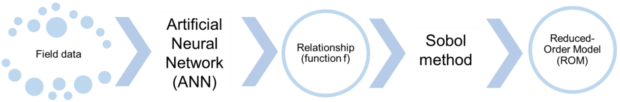
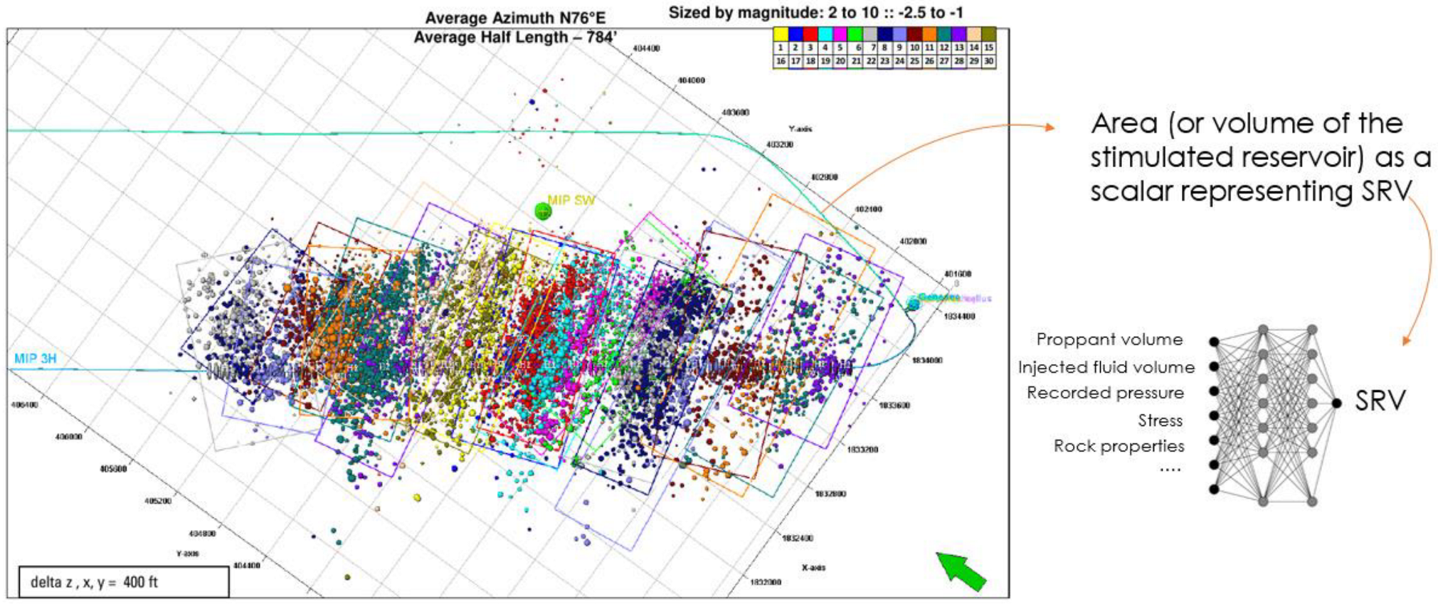
2.1. Data-Based Framework for SRV Prediction

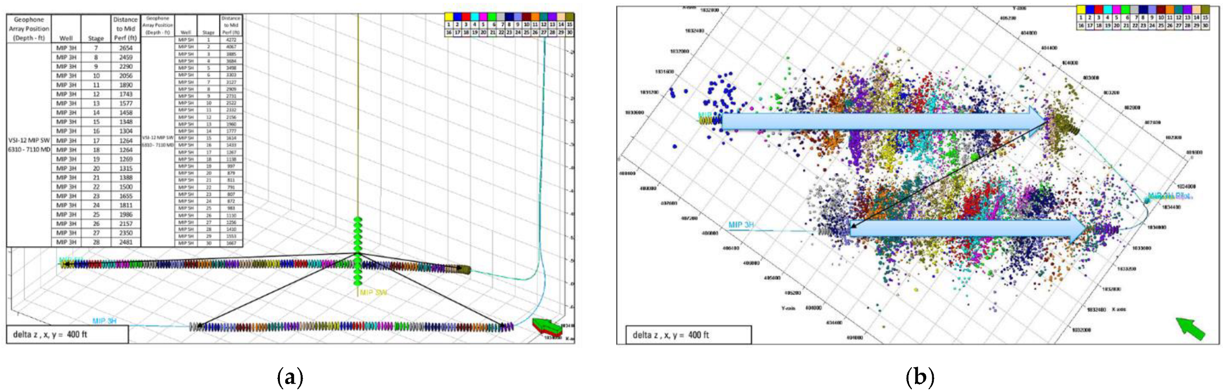
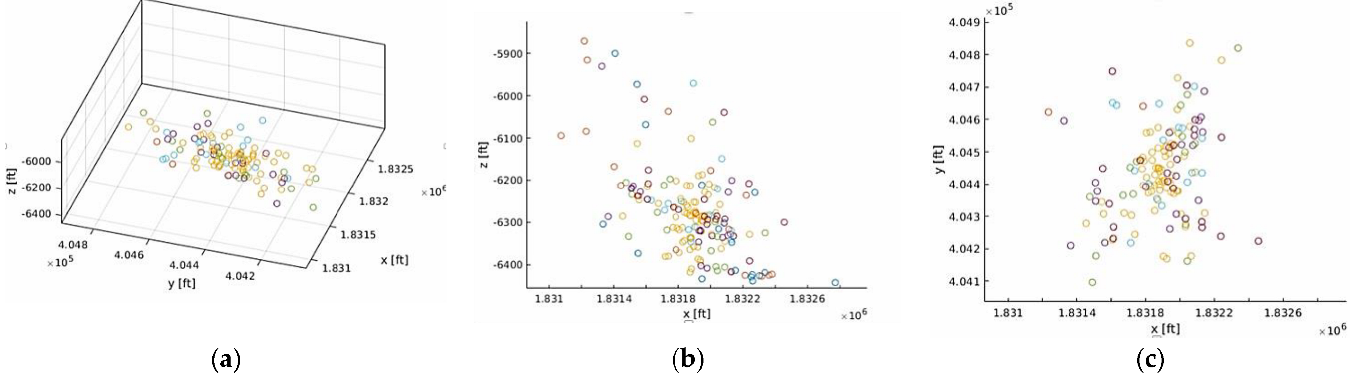
This section discusses the development of several ML models to address some challenging questions regarding the extent of the SRV in the MSEEL. The aim was to use the operational inputs, which could be obtained before or during the wellbore stimulation job. The models presented in this study include KNN, AdaBoost, Random Forest, ANN, and a Stack model to predict the value of the SRV as a single scalar during and after the stimulation job. The models are constructed using the data from two wells in MSEEL. The following section provides a summary of the MSEEL project, the pre-processing, and the steps taken to prepare the data for analysis which is the most time-consuming part of the study. Then, the results of the five ML models are presented. A discussion on the parameters affecting the models’ performance and an approach toward predicting the evolution direction of SRV is also discussed. It should be noted that the python programming language and the Orange software were used for the model developments in this study.

2.1.1. Used Dataset

The dataset used in this study is from MSEEL, an unconventional gas reservoir in the Northeast of the U.S. The MSEEL project aims to provide a long-term field site to develop and validate new knowledge and technology to improve recovery efficiency and minimize environmental implications of unconventional resource development. The project involves several universities, companies, and U.S. research labs for evaluations in geology, geomechanics, completions, production, and completions areas. Figure 2 shows the subsurface and surface information of MSEEL. This project is located in Morgantown, WV. It consists of four horizontal wells, one vertical microseismic monitoring well, and five surface seismic locations. Of the four horizontal wells on the site, there was access to fracturing and microseismic monitoring of wells MIP-3H and MIP-5H. Therefore, the data from these two wells were used for training and testing the ML models.

The two wells are parallel, and the monitoring well was drilled in the spacing between the wells, as shown in Figure 3. Well MIP-3H was stimulated by 28 stages, out of which 22 stages were monitored using microseismic monitoring. In addition, well MIP-5H was fractured using 30 stages, and poor MS monitoring was available at stages greater than 22. Figure 3b shows the location of the MSE, colored by stage. As can be seen, the directions of the microseismic clouds are perpendicular to the well and separate from each other. These clouds are good representatives of SRV.

2.1.2. Model Construction

The volumes (rectangles in 2D) that represent each stage of microseismic activities are shown in Figure 4. SRV at each step (using this approach) is calculated using volumes enclosing most of the microseismic events and represented as the QI. Several input variables, such as proppant volume, fluid volume, average treating pressure, etc., will be used as the model output (Figure 4). It should be noted that each of the hydraulic fracturing stages will be divided into multiple steps containing unique fluid type, proppant concentration, etc. Please also note that the ANN network in Figure 4 is used to illustrate the relationship between input and output variables. Details of the created ML models are discussed in the following sections. An approach for creating more advanced ROM can be to use a combination of datasets generated by simulators and actual data. In this case, each method is intended to generate the required data to make the models in another approach as detailed as possible (fill the missing data). However, limited resources for running the high-fidelity simulators provided access to only the actual field data.

The pre-processing stage included converting the MSEEL reports from pdf format to MS Excel file and combining them as a single file. The variables include stage, step, step name, slurry volume, pump rate, pump time, cumulative pump time (new variable), fluid name, ramp up fluid, proppant name, proppant concentration, proppant mass, average treating pressure, maximum treating pressure, and minimum treating pressure.

Table 1. Input table generated from MSEEL stimulation reports.

Well	Stage	Step	Step Name	Slurry Vol.	Pump Rate	Pump Time	Pump Time Cum.	Fluid Name	Ramp Fluid Vol.	Propp. Name	Propp. Conc.	Propp. Mass	Avg. Treating Press.	Max. Treating Press.	Min. Treating Press.
				bbl	bbl/min	min	min		gal		ppa	lb	psi	psi	psi
MIP-3H	8	1	Rate	20	15	01.30	1.30	1	840	0	0	0	5470	5833	4303
MIP-3H	8	2	Acid	71	15	04.80	6.10	2	2999	0	0	0	6028	6101	5839
MIP-3H	8	3	Pad	595	80	07.40	13.50	1	25,000	0	0	0	7996	9143	6028
MIP-3H	8	4	0.25 PPA	529	80	06.60	20.10	1	22,000	100	0.20	5500	8991	9089	8900
MIP-3H	8	5	0.5 PPA	803	80	10.00	30.10	1	33,000	100	0.50	16,500	8877	8902	8855
MIP-3H	8	6	0.75 PPA	902	80	11.30	41.40	1	36,667	100	0.70	27,500	8913	8948	8893
MIP-3H	8	7	1 PPA	1149	80	14.40	55.80	1	46,200	100	1.00	46,200	8951	8988	8915
MIP-3H	8	8	1.5 PPA	1025	80	12.80	58.60	1	40,333	100	1.50	60,449	9058	9150	8944
MIP-3H	8	9	1.75 PPA	1156	80	14.50	83.10	1	44,982	100	1.80	78,718	9153	9197	9124
MIP-3H	8	10	2 PPA	748	80	09.40	92.50	1	28,812	100	2.00	57,624	9066	9200	8361

shows a few examples of these variables for stage 8 of MIP-3H. In the table, the concept of steps is shown. Basically, a step is a substep of a stage with unique properties. This approach also helped to increase the sample number to ~800 and apply a model that can predict the SRV volume in near-real-time. Moreover, a new variable called cumulative pump time is created in the table to relate the input variables at each step. Later, this new variable will be used to correlate the observed MS events to the pump schedule.

Table 2. The generated table for MS.

Well	Stage	Step	Time	Time Difference	Cum. Time	YLoc	XLoc	TVD (Z)
						Ft	Ft	Ft
MIP-5H	2	1	10:30:10	00:00:00	00:00:00	407,735.31	1,831,598.25	−5986
MIP-5H	2	1	10:30:34	00:00:24	00:00:24	407,753.94	1,831,645.44	−5968
MIP-5H	2	1	10:30:41	00:00:07	00:00:31	407,653.12	1,831,692.37	−6271
MIP-5H	2	2	10:32:38	00:01:57	00:02:28	407,590.36	1,831,319.54	−5865
MIP-5H	2	3	10:37:08	00:04:30	00:06:58	407,606.55	1,831,496.50	−5840
MIP-5H	2	3	10:44:45	00:07:37	00:14:35	1,831,301.72	407,706.51	−6135
MIP-5H	2	7	11:01:14	00:16:29	00:31:04	1,831,879.96	407,641.13	−5475
MIP-5H	2	9	11:11:24	00:10:10	00:41:14	1,831,688.69	407,965.96	−6320
MIP-5H	2	9	11:11:53	00:00:29	00:41:43	1,831,600.45	408,043.02	−6503
MIP-5H	2	9	11:14:01	00:02:08	00:43:51	1,831,564.41	407,803.99	−6201

shows the generated output table from the recorded microseismic events. The data contained the x, y, and z location of the events and their magnitude. However, the magnitudes were excluded from this study and can be used later for adjusting the calculated SRV. Cumulative time (from the start of fracking) columns were created in the output table, similar to the cumulative time from the input table. In that period, all recorded microseismic events were assigned to the corresponding input step, and the volume of a geometrical shape enclosing the points was calculated as DSRV. Next, a wrapper file was created to loop through the stage, step, and cumulative time, find the corresponding MS events for that specific step, and calculate the SRV.

This approach resulted in a group of distinguished MS events for each step. Figure 5 shows an example of such grouping for MIP-3H stage 7. Note that the MS events are color-coded for each step (note: the steps are smaller periods inside each stage). Also note that two parameters are changing from one step to another. These parameters are the extent of the SRV and its enclosing points (i.e., the density of the MS events in the enclosed geometry). This study focused only on estimating the extent of the SRV. However, it is critical to consider the density of the changes in the SRV, valuable information that can be obtained from the MS points in the plots, and the direction of the SRV growth. For example, the direction of SRV growth is NW–SE and NE–SW in the 2D plots shown below. The SRV direction can be further analyzed to track the evolution of the SRV in near-real-time.

As was mentioned, the last step towards creating the output parameter (i.e., SRV) is estimating a volume enclosing the MS events. For this purpose, a threshold may be devised that eliminates the isolated MS events and does not seem to contribute to the overall SRV estimations. This study enclosed all points in an irregular geometry, and later in the cleaning data section, the samples with volumes much bigger than a certain threshold are removed from the dataset. Figure 6 shows two examples of the estimated SRV for MIP-3H stage 7 and MIP-5H stage 12. The volumes that are calculated as SRV are color-coded for the steps.

Once the SRVs (or DSRV) are known for each step, they are added to the input table as a new column and used as our target variables. The next step toward building the ML models was to perform some exploratory data analysis to find the relationship between the input parameters and their relationship with the output parameters. This was performed in several ways. An example is plotted in Figure 7. This study started with all 15 variables that were available in the input table. As shown in the confusion matrix, several relationships were identified between the input samples. For example, average, max, and min pressures have similar effects on the SRV, as highlighted in green boxes. In addition, some variables seem to have linear correlation (see, for example, ramp-up fluid volume and slurry volume). Moreover, some of the inputs resulted in multiple SRVs (e.g., pump rate) and could negatively impact the model performance. Finally, some of the variables have outliers that need to be removed. An example of this case is the estimated SRV, as explained previously. Some of the SRV values were considerably bigger than the others, indicating the non-productive MS events.

As a result, some of the mentioned columns were removed from the input features, and some were corrected by removing outliers to avoid any model bias (Figure 8). Finally, eight parameters were selected from the analysis performed in the previous step. The final input/output table is shown in

Table 3. The final set of input/output. The maximum calculated SRV in this study is about ~14 times bigger than what was reported in Barnett shale [26].

	Well	Stage	Step	Slurry Volume	Pump Time	Pump Time Cum.	Propp. Conc.	Propp. Mass	Avg. Treating Press.	SRV (Estimated)
				bbl	min	min	PPA	lb × 103	psi	ft3
Min	-	1	1	-	-	0	0	-	5000	0
Max	-	26	24	1500	20	160	4	100	9000	3 × 108

. The parameter “well name” is selected metadata. The input columns used to create the models were stage, step, slurry volume, pump time, cumulative pump, proppant concentration, proppant mass, and average treating pressure. Note that some of the SRVs in the output column are zero, indicating no creation of SRV. Some of these rows with zero SRV were also removed from the data, especially if they were in the middle of the stage, where the pump rate and prop concentrations were maximum (it was assumed that the high injection rate should result in some SRV creation, especially if the steps before or after created SRV). The zero SRV can be related to an error in MS monitoring or not creating an SRV (smaller chance).

After all the changes were made to the initial data, 582 samples remained. The remaining samples were then grouped into 482 and 100 samples (80/20) for training and testing. It should also be noted that the data was shuffled and normalized to a [0, 1] interval before creating the ML models.

A heat map of the selected input variables is shown in Figure 9. As can be seen, the parameters that affect the output parameters the most are slurry volume, pump time, and proppant mass. In addition, the least affecting parameters are stage and prop concentration. Moreover, the relationship between pump time and slurry volume has strong correlation weights in modeling, as shown in the figure.

Five different ML models were trained and tested on the processed data table. The models are AdaBoost, KNN, Random Forest, AAN, and a stack model including the Random Forest, KNN, and AdaBoost. For the KNN model, the number of neighbors, metric, and weight were set as five; Euclidian and distance were set as the model parameters. The AdaBoost model used the number of estimators and learning rate of 100 and 1, respectively. In addition, SAMM.R [27] classification algorithm and exponential regression loss function were used. For the Random Forest model, the number of trees was set as 500, the number of attributes at each split as 7, and limited the depth of individual trees to 20. Moreover, three hidden layers were used with 80 nodes each for the ANN model, the ReLu activation function, and the Adam optimizer. Furthermore, the regularization was set as 0.01 and the maximum number of iterations as 100. Lastly, the created Random Forest, KNN, and AdaBoost were used as the learners of the Stack model. In addition, the Ridge Regression algorithm was used for aggregating the input models. The selection of all of the mentioned hyperparameters was based on experimentation of the model performance on the test set. The performance of these algorithms is discussed in the results and discussion section.

2.2. Global Sensitivity Analysis and Reduced Order Model

A ROM has the following properties: (1) it is a mathematically simple function that maps a set of input variables to QI (i.e., SRV in the current study), (2) it can replace the original function, and (3) its error compared to the original model can be controlled. The actual function may be known, mathematically complicated, or unknown. This technique may be applied to pure data- and physics-based models. This paper used the [17] method to produce the final ROM from the created data-based models. The technique is a powerful global sensitivity analysis method, which can also be used to build ROMs. The term ROM is used in this paper to refer to simple mathematical equations that relate input parameters of a known (or unknown) function to an output QI. These mathematical equations can replace the primary function with a controlled error. Creating ROM from raw field data can be extremely helpful from several perspectives. ROMs may be used in simple software packages by the field engineers (e.g., MS Excel) to cross-validate solutions obtained by other methods or replace them. Solutions to these functions are typically obtained faster than the original function. Therefore, they can be used for real-time decision-making. For example, a reasonably complex problem requiring several hours of numerical calculations can be obtained in a few seconds with the corresponding ROM.

2.2.1. The Mathematical Background of the Sobol Method

The mathematical formulation of the Sobol technique for an arbitrary function $f$ (ML models discussed in the previous section) is summarized as follows [17]:

$$y=f\left(x\right)$$

(1)

where $x$ is a set of input parameters on the n-dimensional hypercube such that:

$${\mathsf{\Omega }}^n:=\left\{x|0\le x_i\le 1,i=1,\dots ,n\right\}$$

Function $f$ can be written as the ANAVO representation (abbreviated from Analysis of Variance) as:

$$f\left(x\right)=f_0+{\displaystyle \sum }_{s=1}^n{\displaystyle \sum }_{i_1<\dots <i_s}^n{f}_{i_1\dots .i_s}\left(x_{i_1},\dots ,x_{i_5}\right), 1\le i_1<\dots <i_s\le n,$$

(2)

One may rearrange the previous equation to obtain a series of increasing order Sobol functions as follows:

$$f\left(x\right)=f_0+{\displaystyle \sum }_{i=1}^n{f}_i\left(x_i\right)+{\displaystyle \sum }_{i=1}^n{\displaystyle \sum }_{j=i+1}^n{f}_{ij}\left(x_i,x_j\right)+\dots +f_{i\dots n}\left(x_1,\dots ,x_n\right)$$

(3)

The following statements should be satisfied to make the above equation applicable:

• f₀ should be constant.
• The integral of each member over its variables = 0

$${{\displaystyle \int }}_0^1{f}_{i_1\dots i_s}\left(x_{i_1},\dots ,x_{i_5}\right)d{x}_k=0 \forall k=i_1,\dots .,i_s$$

(4)

3

All the terms in Equation (3) are orthogonal, meaning that if (i₁,..., i_s) ≠ (j₁,…, j_t), then

$${{\displaystyle \int }}_{{\mathsf{\Omega }}^n}^{ }{f}_{i_1\dots .i_s} f_{j_1\dots .j_t}dx=0$$

(5)

where

$$f_0={{\displaystyle \int }}_{{\mathsf{\Omega }}^n}^{ }f\left(x\right)dx=0$$

(6)

$$f_i\left(x_i\right)={{\displaystyle \int }}_{{\mathsf{\Omega }}^n}^{ }f\left(x_i,x_{~i}\right)d{x}_{~i}-f_0$$

(7)

$$f_{ij}\left(x_i,x_j\right)={{\displaystyle \int }}_{{\mathsf{\Omega }}^{n-2}}^{ }f\left(x_i,x_{j,}{x}_{~ij}\right)d{x}_{~ij}-f_0-f_i\left(x_i\right)-f_j\left(x_j\right)$$

(8)

where $x_{\sim i}$ is the vector corresponding to all variables except $x_i$ in the input set $x$, and $x_{\sim ij}$ is the vector corresponding to all variables except $x_i$ and $x_j$ in the input set $x$. Assuming that $f\left(x\right)$ is square-integrable, the total variance of $f$ is given by:

$$D=V\left[f\right]={{\displaystyle \int }}_{{\mathsf{\Omega }}^n}^{ }{f}^2\left(x\right)dx-f_0^2={\displaystyle \sum }_{s=1}^n{\displaystyle \sum }_{i_1<\dots <i_s}^n{f^2}_{i_1\dots i_s}\left(x_{i_1},\dots ,x_{i_5}\right)d{x}_{i_1}\dots . d{x}_{i_s}$$

(9)

Equation (9) can also be written in terms of the partial variances of $f$ as:

$$D={\displaystyle \sum }_{s=1}^n{\displaystyle \sum }_{i_1<\dots <i_s}^n{D}_{i_1\dots .i_s}={\displaystyle \sum }_{i=1}^n{D}_i+{\displaystyle \sum }_{i=1}^n{\displaystyle \sum }_{j=i+1}^n{D}_{ij}+\dots .D_{1\dots n}$$

(10)

where $D_i$, $D_{ij}$,…., $D_{i\dots j}$ can be calculated by integrating the corresponding Sobol functions as follows:

$$D_i={{\displaystyle \int }}_{{\mathsf{\Omega }}^1}^{ }{f}_i^2\left(x_i\right)d{x}_i$$

(11)

$$D_{ij}={{\displaystyle \int }}_{{\mathsf{\Omega }}_2}^{ }{f}_{ij}^2\left(x_i,x_j\right)d{x}_{i}d{x}_j$$

(12)

$$D_{i_1\dots .i_s}={{\displaystyle \int }}_{\mathsf{\Omega }}^{ }{f}_{i_1\dots i_s}^2\left(x_{i_1}, \dots ,x_{i_s}\right)d{x}_{i_1}\dots d{x}_{i_s}$$

(13)

From the descriptions, Sobol indices are the ratio of the partial variances to the total variance as:

$$S_i=\frac{D_i}{D}$$

(14)

$$S_{ij}=\frac{D_{ij}}{D}$$

(15)

$$S_{i_1\dots i_s}=\frac{D_{i_1\dots i_s}}{D}$$

(16)

In this preparation, higher indices mean a higher effect on the variation of the output parameter. In addition, Sobol indices are non-negative indices that have the following property:

$${\displaystyle \sum }_{s=1}^n{\displaystyle \sum }_{i_1<\dots <i_s}^n{S}_{i_1\dots .i_s}={\displaystyle \sum }_{i=1}^n{S}_i+{\displaystyle \sum }_{i=1}^n{\displaystyle \sum }_{j=i+1}^n{S}_{ij}+\dots .S_{1\dots n}=1$$

(17)

Sobol indices allow for conducting evaluations according to their Sobol indices to order input variables.

2.2.2. Sobol Method for Complex Functions

For functions that are not polynomials, a Monte Carlo integration is necessary to calculate the integrals required by Sobol analysis [18]. Sobol functions can be calculated as follows:

$$\overline{f_0}=\frac{1}{N}{\displaystyle \sum }_{m=1}^{N}f\left(x_m\right)$$

(18)

$$\overline{D}=\frac{1}{N}{\displaystyle \sum }_{m=1}^N{f}^2\left(x_m\right)-{\overline{f_0}}^2$$

(19)

$$\overline{D_i}=\frac{1}{N}{\displaystyle \sum }_{m=1}^{N}f\left(x_m\right)f\left(x_{im},x_{~im}^c\right)-{\overline{f_0}}^2$$

(20)

$$\overline{D_{ij}}=\frac{1}{N}{\displaystyle \sum }_{m=1}^{N}f\left(x_m\right)f\left(x_{im},x_{~im}^c\right)-\overline{D_i}-\overline{D_j}-{\overline{f_0}}^2$$

(21)

where $m$ is the test number, and $N$ is the sample size of the inputs.

Figure 1 showed the central idea of the approach to creating ROM for estimating SRV from field observations used in this study. As explained in the previous sections, several ML models were created to predict the SRV as a scalar in a dynamic fashion (i.e., DSRV). The ML models are used separately as the $f$ function in Equations (1) and (18). However, the reported ROM in this write-up is built using the AdaBoost model. Then, using the Sobol method, this study first identifies the importance of the input parameters in the ANN models. As stated before, the advantage of the Sobol method in ranking the input parameters is that it can account for interaction terms. Finally, the ROM is built using the most dominant input parameters.

3. Results and Discussion

The hydraulic fracturing process is typically executed one stage at a time from the toe of the horizontal to the heel. At each stage, a certain amount of fracturing fluid is injected into the wellbore to break the rock and create new surfaces in the reservoir that can help increase the conductivity (k × w) and hydrocarbon flow toward the wellbore from the stimulated region. As a result of this injection and depending on several variables such as the amount of injected fluid, local stress in the rock, and natural fracture density and orientation of the natural fractures in the pay zone, different “SRV” sizes are generated. The SRV extent is usually tracked using three different methods: direct far-field, direct near-wellbore, and indirect fracture diagnostics [28]. The direct far-field techniques are suited to give the global visual perspective about fracture growth and are conducted in a separate well. Tiltmeter and microseismic fracture mapping are the two commonly used techniques for this type of fracture diagnostics.

On the contrary, the second group of fracture diagnostics techniques is implemented in the same well. It gives information about near-wellbore fracture parameters such as height, width, and proppant placement. Finally, the most used fracture diagnostics group is indirect fracture diagnostics. The techniques used in this group can provide estimates of fracture conductivity, dimension, and stress. This group includes fracture design model optimization, pressure transient testing, and production data analysis [28].

The multistage hydraulic fracturing process simulation is tedious and requires high-fidelity models for many reasons. As mentioned, this study used the available data collected while or before performing hydraulic fracturing as input. These variables include fracturing fluid type, rate, treating pressure, and proppant properties. On the output side, a volume enclosing the microseismic events (MSE) from hydraulic fracturing processes is estimated and used as the output variable.

A function that maps a set of inputs to output parameters is needed to create the ROM. In the case of SRV prediction, such a function needs to map the hydraulic fracturing parameters such as pump rate and proppant volume to the volume and growth direction of the SRV. The function need not be known explicitly. Possible options for such a prediction could be high-fidelity physics-based models, data-driven models, or a combination of both, also known as hybrid models. A high-fidelity numerical simulator can be used to generate the synthetic data required for creating ROM. In this case, an example is to use GEOS [29] to (1) match the hydraulic fracturing operation in the two MSEEL wells and (2) generate the dataset required for the Monte Carlo simulation. Then, a similar approach to the one discussed in the later sections of the paper can be used to construct the ROM. Figure 10 shows an example of the applicability of GEOS for this purpose. In this example, because of a hydraulic fracture propagation into a naturally fractured reservoir, a microseismic map is generated that can be used to estimate SRV.

It is essential to characterize and map fractures and fracture networks, including their topological evolution during stimulation and the hydrocarbon flow through them over time. Such a characterization is possible through the concept of SRV. The term “fracture” in the above discussions is used to present rock discontinuities in the macroscopic scale (i.e., $\mathrm{cm}$ to $\mathrm{m}$). These fractures can be in the form of induced or pre-existing. They can also take or do not take fluid; however, they all have two distinct surfaces that can move in shear and tensile modes with respect to each other. In addition, the length of these fractures may change due to pressure/stress changes in the reservoir and fracture. The conductive network of fractures (induced and pre-existing) that can take fluid and are connected is referred to as SRV and is of particular interest from the hydrocarbon production aspect. The following section discusses the results of the data-based models and then performs a GSA. Finally, the ROM is constructed based on the dominant parameters from the GSA.

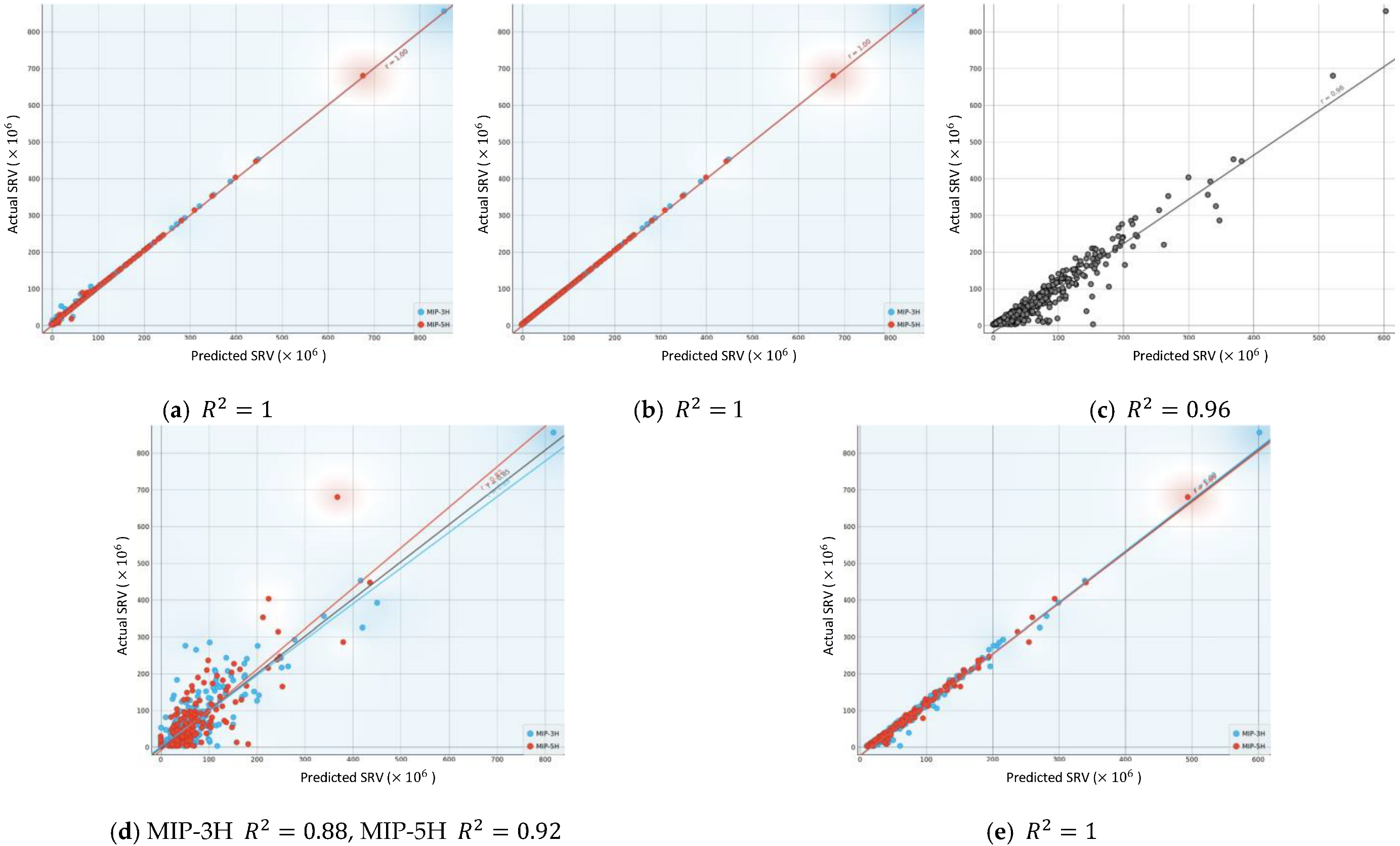
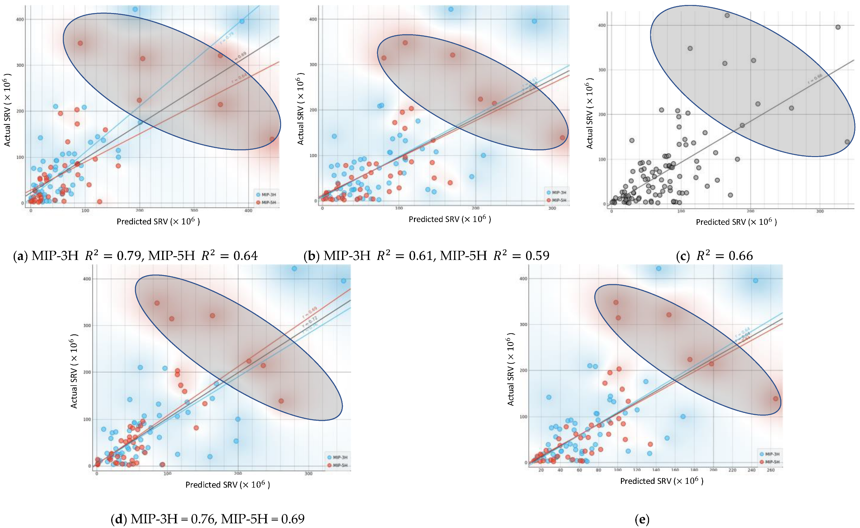
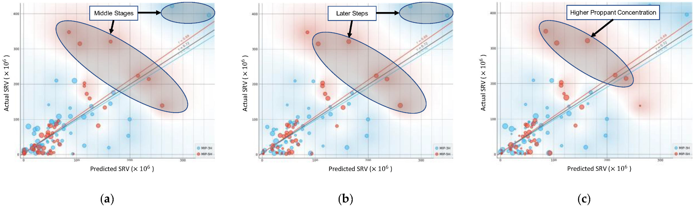
3.1. ML Models Performances

The created models’ performances on the training set, including 482 samples, are shown in Figure 11. The x-axis on the plots shows the predicted values of the SRV, and the y-axis shows the original value from the test set. In addition, the line on the plots shows the R-Square of each model. Moreover, the points are color-coded based on the well number. Please note that the model’s performance on the training set should not be used as a metric for model performance. As can be seen, the R-square for AdaBoost, KNN, and stack is 1 for the train set, while Random Forest and ANN have R-squares of 0.96 and 0.85 (overall). All models perform slightly better on the well MIP-3H compared with MIP-5H. The reason might be that the number of data samples in MIP-5H was smaller, and there was an error for several points in the middle stages. More discussions will be provided on this point later in this section.

The test data included 100 data samples from both wells. Figure 12 shows the model performance of the models on the test set. As expected, the performance is lower on the test model. Again, the results are color-coded for the well number and show that the model performance is generally better for MIP-3H. The overall R-square for test sets are 0.69, 0.60, 0.68, 0.72 and 0.64 for AdaBoost, KNN, Random Forest, and Stack models, respectively. As can be seen, among all models, ANN had a better performance on the test set with a 0.72 R-square. The model’s performance may be improved by adding more training samples and details about the target formation properties. For example, an idea about the distribution, density, and orientation of natural fractures may help better predict the SRV. One reason for lower overall R-squares is the lower performance on well MIP-5H, which is caused by the poor prediction of six points. The points are highlighted in the figure with a yellow shaded area. This weak performance could be an error in data collection or weak engineering or execution of the fracturing job in that stage. To further investigate the reason behind models’ weak performances on these six points, another investigation was performed on the mentioned points, and the results are discussed next. Note that other metrics may be used to evaluate the performances of the models, but they have been skipped in this study.

To further investigate the reason for the weak performance of the models, the results are plotted as a function of three variables, namely, stage number, step, and proppant concentration. For this purpose, the AdaBoost model was arbitrarily selected. However, the six points were observed in other models as well. Figure 13 shows the results for the three selected variables. In this presentation, the size of each bubble represents the magnitude of the selected variable. For example, a bigger circle means the stage number is bigger (i.e., closer to the heel). Figure 13a shows the results for stage number. As can be seen, the incorrectly predicted points are all from the stage in the middle of the well. It can also be concluded that the steps in five points are toward the end of the fracturing job for that specific stage, where the pump rates and proppant concentrations were the highest. Figure 13 confirms this observation. Five of the incorrectly predicted points were from high proppant concentrations in that figure. More investigations may be conducted to further analyze the poor model performance in these six points.

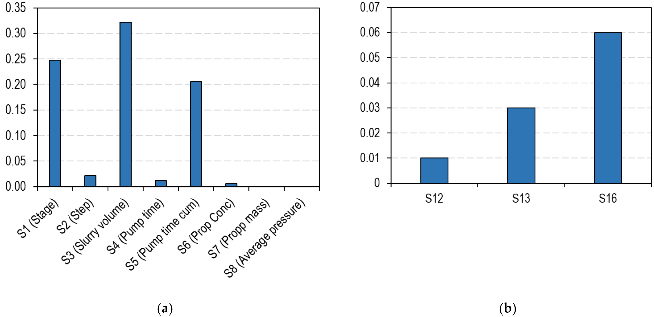
3.2. Global Sensitivity Analysis on Parameters Affecting the SRV

In both physics- and data-based approaches discussed in the previous sections, a Monte Carlo simulation is required to create the ROM since the governing function is not known. Therefore, a set of input data (variables) and an output QI should be generated. This study used the AdaBoost model, hereafter, for performing the analysis. The eight parameters that were used for creating the ML models were used here as well. The first step toward generating any data-based ROM with real-time prediction capabilities is to identify the dominant parameters that affect the variation in the output parameter. The function may later be used to create a ROM that can predict the QI in real-time.

A Monte Carlo simulation using 180,000 combinations from the input variables (c.f., Table 3) was created and used in the ML model to generate the QI (i.e., DSRV). The ranges of parameters are given in Table 3. The Sobol technique was then applied to the set to estimate the corresponding indices. This analysis was limited to second-order indices and neglected higher-order indices (it will become obvious later that they are negligible). Figure 14 shows the first- and second-order Sobol indices. As seen in the figure, among the first order Sobol indices, the slurry volume (i.e., S3) has the most significant effect (~0.32) on SRV. This means that 32% of changes in SRV predictions using the created ML model come from the slurry volume alone. The second and third most dominant variables among first-order indices are the stage number and pump time with 25% and 21%, respectively. Figure 14b shows the Sobol indices of the second-order indices of the input variables. For example, S13 is the Sobol index related to the simultaneously changing variables S1 and S3. As shown in the figure, S16 has the most dominant effect among the rest of the second-order indices (~6%). As mentioned, higher-order Sobol indices, such as $S_{123}$, were neglected. The main reason for ignoring those terms is that the summation of the considered indices up to second order adds up to >90% of the changes in the estimated SRV. If more precise results are desired, one can include the higher-order terms with the same methodology described above. Based on the results in this section, one may represent ~90% of the changes in the pressure drop by considering the following Sobol indices:

$$S_1+S_2+S_3+S_5+S_{13}+S_{16}=0.9 \mathrm{of} \mathrm{the} \mathrm{SRV} \mathrm{calculated} \mathrm{from} \mathrm{the} \mathrm{ML} \mathrm{model}$$

Therefore, these four variables and some of their second-order interactions are used to create the ROM.

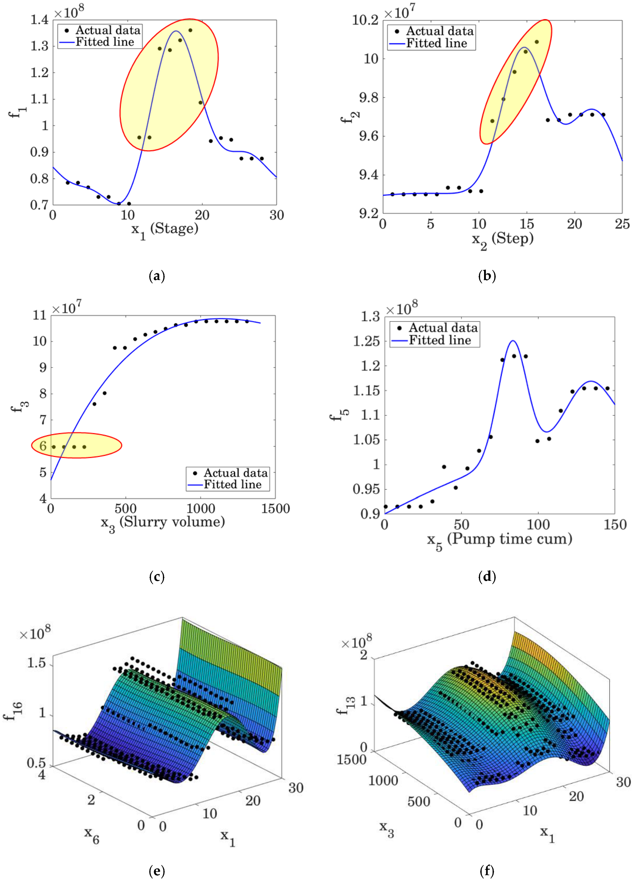
3.3. ROM for Predicting SRV Using Recorded Field Data

This section presents the creation of the ROM by applying the Sobol method to the dominant variables discussed in the last section. The ROM can be used to predict the SRV (same as the ML model) and has two main advantages over the numerical and data-based models: (1) it can replace the simulations with a relatively simple mathematical function and a reasonable accuracy, and (2) the CPU run time can be reduced significantly. Since the governing function for estimating the SRV from hydraulic fracturing parameters is not known, a Monte Carlo simulation is used to carry out some of the required integrations. Figure 15 shows the results for first- and second-order Sobol functions obtained by this approach. The y-axis of the plots has the same dimension as SRV (i.e., $L^3$) and indicates the changes in the estimated SRV from the corresponding input variable. As shown in the figure, the estimated SRV changes tremendously for the stages in the middle of the well for an unknown reason. This behavior change could be due to the lack of engineering design, erroneous MS recording, or uncertainty in the target formation properties. In addition, it is observed that for the first few initial steps, the estimated SRV does not change much. However, the estimation changes significantly for the steps where the pump rate reaches its maximum and proppant concentration is high. Similar trends could be observed for slurry volume and cumulative pump time.

To obtain the mathematical expression of the scatter plots, fit functions (solid blue line in single-term functions and surface in double-term functions) are used. The fit can then be used to replace the integrations that are required for constructing the ROM.

Using the fit functions that were obtained in the previous section and Equation (3), one can construct the ROM. For this purpose, the Sobol functions need to be built using the individual and second-order fit function. The summary of the Sobol functions is shown in

Table 4. The reduced-order functions for estimating SRV using input variables.

Function	Mathematical Form
$F_0$	$f_0$
$F_1$	$f_1-F_0$
$F_2$	$f_2-F_0$
$F_3$	$f_3-F_0$
$F_5$	$f_5-F_0$
$F_{13}$	$f_{13}-F_1-{\mathrm{F}}_3-{\mathrm{f}}_0$
$F_{16}$	$f_{16}-F_1-{\mathrm{F}}_6-{\mathrm{f}}_0$

. The lower-case $f$ functions in the table refer to fit functions, and upper-case $F$ functions refer to the Sobol functions.

Based on the presented results, the reduced-order function for predicting the SRV can be written as:

$$SRV=F_0+F_1+F_2+F_3+F_5+F_{13}+F_{16}$$

(22)

The presented ROM can replace the complex high-fidelity models and the created ML models for estimating SRV. The associated error to this ROM should be about 10% with respect to the AdaBoost model that was used.

3.4. Steps to Improve the Models

Two variables control the created SRV: operational parameters and rock geomechanical and mineralogical variables. Operational parameters include pump schedule (e.g., duration, rate), recorded pressure, and perforation design. However, rock-related parameters include rock mineralogy, stress state, natural fracture properties such as density and orientation relative to the wellbore direction, layer height in the pay zone, etc. This study only limited the operational parameters because of limited data availability. Including the rock-related parameters will improve the performance of the models. In addition, the number of examples in this study was relatively small (580), and adding more examples is expected to improve the performance. Another approach that one may take to improve the performance of these models is to apply some unsupervised learning algorithms to the data. For example, Figure 16 shows the result of the self-organizing map (SOM) on different properties. The algorithm can be used to cluster the input data based on some variables. The figure applies the algorithm to mesh size, fluid type, and proppant concentration in the figure, as can be seen. For example, in Figure 16b, the samples with WF115 seem to have similar behavior. In addition, the points show similar behavior when the proppant concentration is less than one bb/gal (Figure 16c). This clustering helps to further decrease the model errors.

Another parameter that was ignored in this study was MS events magnitude. The magnitude of the events plays a role in the intensity of permeability changes in the stimulated zone. In future studies, this property will be included in models. In addition, one important aspect of the SRV evolution is its growth direction. The fractures will not always propagate symmetrically. The fracture propagation direction can be affected due to stress shadowing from previous steps or layer confinement in height. Another idea to further address the evolution direction of SRV is the quadrant idea. This approach divides a sphere (in 3D) into multiple equal-sized quadrants. Suppose the frac fluid is injected at the point center of a sphere, and the reservoir rock is uniformly diffusive to fluids expanding radially. In that case, the sphere can be a proxy shape for isotropic, homogenous reservoir rock. However, this is not always the case. Figure 17 shows the quadrant idea. In this approach, one needs to start with a small circle centered at the wellbore (Figure 17b). A new circle is drawn from the same center with a bigger radius at each step. By tracking the number of points in each quadrant, one may estimate the evolution direction of SRV. For example, more points are in the three quadrants of NE, NE, and SW of the example in Figure 17. Therefore, it may be concluded that the SRV is blocked from propagating in the NW quadrant. A look at the design and location of the wheels with geological data will be a helpful addition to this analysis to determine the reason.

4. Conclusions

This paper summarized the following developments: (1) a data-driven model to dynamically predict the SRV, and (2) a ROM for predicting the SRV. The SRV in this approach is called DSRV and can be used for real-time analysis of the induced stimulated zone evolution. Each hydraulic fracturing stage has been broken down into several steps in this approach, each having unique properties such as pump rate, proppant concentration, and average treating pressure. These properties were used in the input feature table. A data set from the MSEEL project, including 58 stages from two wells (MIP-3H and 5H), was used. On the output side, irregular geometrical shapes were automatically created around each recorded microseismic cloud at each step and represented as SRV. Then the time of each step was correlated to the SRV volume to make the required table for the model creation. Several ML models were implemented on the data, including AdaBoost, KNN, ANN, Random Forest, and a stack algorithm. The models had an R-Square metric of 0.65–0.78 on the test data, which is an acceptable range for such a limited dataset. The performance of the models can be improved by adding more training examples (this study only used ~500 samples). Models showed weaker performance in the middle stages of MIP-5H, negatively impacting the overall performance. This study also proposed two approaches to estimate the evolution of SRV: volume prediction and quadrant. The volume prediction in real-time was presented in this study. In future models, the quadrant idea to estimate the growth direction of SRV can be included. Model performances can be improved by adding more data samples and information about the target formation. Also, the MS events’ magnitudes will be included to better estimate SRV. For the ROM, Sobol GSA was used. First, the technique to identify the dominant variables was used. It was observed that Stage number, step number, slurry volume, pump time, and their combinations account for 90% of the ML model predictions.

References

1. Wang, S.; Qin, C.; Feng, Q.; Javadpour, F.; Rui, Z. A framework for predicting the production performance of unconventional resources using deep learning. Appl. Energy 2021, 295, 117016. [Google Scholar] [CrossRef]
2. Wang, S.; Chen, S. Insights to fracture stimulation design in unconventional reservoirs based on machine learning modeling. J. Pet. Sci. Eng. 2019, 174, 682–695. [Google Scholar] [CrossRef]
3. Siddiqui, F.; Rezaei, A.; Dindoruk, B.; Soliman, M.Y. Eagle ford fluid type variation and completion optimization: A case for data analytics. In Proceedings of the SPE/AAPG/SEG Unconventional Resources Technology Conference, Denver, CO, USA, 22–24 July 2019. [Google Scholar]
4. Luo, G.; Tian, Y.; Bychina, M.; Ehlig-Economides, C. Production optimization using machine learning in Bakken shale. In Proceedings of the Unconventional Resources Technology Conference, Houston, TX, USA, 23–25 July 2018; Society of Exploration Geophysicists, American Association of Petroleum Geologists, Society of Petroleum Engineers: Tulsa, OK, USA; pp. 2174–2197. [Google Scholar]
5. Chen, X.; Li, J.; Gao, P.; Zhou, J. Prediction of shale gas horizontal wells productivity after volume fracturing using machine learning—An LSTM approach. Pet. Sci. Technol. 2022, 40, 1861–1877. [Google Scholar] [CrossRef]
6. Srinivasan, S.; O’Malley, D.; Mudunuru, M.K.; Sweeney, M.R.; Hyman, J.D.; Karra, S.; Frash, L.; Carey, J.W.; Gross, M.R.; Viswanathan, H.S. A machine learning framework for rapid forecasting and history matching in unconventional reservoirs. Sci. Rep. 2021, 11, 21730. [Google Scholar] [CrossRef] [PubMed]
7. Zhao, P.; Gray, K.E. Analytical and Machine-Learning Analysis of Hydraulic Fracture-Induced Natural Fracture Slip. SPE J. 2021, 26, 1722–1738. [Google Scholar] [CrossRef]
8. Urban-Rascon, E.; Aguilera, R. Machine Learning Applied to SRV Modeling, Fracture Characterization, Well Interference and Production Forecasting in Low Permeability Reservoirs. In Proceedings of the SPE Latin American and Caribbean Petroleum Engineering Conference, OnePetro, Virtual, 27–31 July 2020. [Google Scholar]
9. Sprunger, C.; Muther, T.; Syed, F.I.; Dahaghi, A.K.; Neghabhan, S. State of the art progress in hydraulic fracture modeling using AI/ML techniques. Model. Earth Syst. Environ. 2021, 8, 1–13. [Google Scholar] [CrossRef]
10. Tandon, S. Improved Analysis of Stimulated Reservoir Volumes in Unconventional Reservoirs Using Supervised Learning Techniques. In Proceedings of the SPE Eastern Regional Meeting, Charleston, WV, USA, 15–17 October 2019. [Google Scholar]
11. Wang, L.K.; Sun, A.Y. Well Spacing Optimization for Permian Basin Based on Integrated Hydraulic Fracturing, Reservoir Simulation and Machine Learning Study. In Proceedings of the SPE/AAPG/SEG Unconventional Resources Technology Conference, Virtual, 20–22 July 2020. [Google Scholar]
12. Lecampion, B.; Desroches, J.; Weng, X.; Burghardt, J.; Brown, J.E. Can we engineer better multistage horizontal completions? Evidence of the importance of near-wellbore fracture geometry from theory, lab and field experiments. In Proceedings of the SPE Hydraulic Fracturing Technology Conference, The Woodlands, TX, USA, 3–5 February 2015. [Google Scholar]
13. Morozov, A.D.; Popkov, D.O.; Duplyakov, V.M.; Mutalova, R.F.; Osiptsov, A.A.; Vainshtein, A.L.; Burnaev, E.V.; Shel, E.V.; Paderin, G.V. Data-driven model for hydraulic fracturing design optimization: Focus on building digital database and production forecast. J. Pet. Sci. Eng. 2020, 194, 107504. [Google Scholar] [CrossRef]
14. Rafiee, M.; Rezaei, A.; Soliman, M. Investigating hydraulic fracture propagation in multi well pads: A close look at stress shadow from overlapping fractures. Hydraul. Fract. J. 2015, 2, 23–27. [Google Scholar]
15. Saltelli, A.; Tarantola, S.; Campolongo, F.; Ratto, M. Sensitivity Analysis in Practice: A Guide to Assessing Scientific Models; John Wiley & Sons: Hoboken, NJ, USA, 2004. [Google Scholar]
16. Saltelli, A.; Ratto, M.; Andres, T.; Campolongo, F.; Cariboni, J.; Gatelli, D.; Saisana, M.; Tarantola, S. Global Sensitivity Analysis: The Primer; John Wiley & Sons: Hoboken, NJ, USA, 2008. [Google Scholar]
17. Sobol, I.M. Sensitivity estimates for nonlinear mathematical models. Math. Model. Comput. Exp. 1993, 1, 407–414. [Google Scholar]
18. Sobol, I.M. Global sensitivity indices for nonlinear mathematical models and their Monte Carlo estimates. Math. Comput. Simul. 2001, 55, 271–280. [Google Scholar] [CrossRef]
19. Rezaei, A.; Nakshatrala, K.B.; Siddiqui FA, H.D.; Dindoruk, B.; Soliman, M. A global sensitivity analysis and reduced-order models for hydraulically fractured horizontal wells. Comput. Geosci. 2020, 24, 995–1029. [Google Scholar] [CrossRef] [Green Version]
20. Kumar, A.; Hu, R.; Walsh, S.D. Development of Reduced Order Hydro-mechanical Models of Fractured Media. Rock Mech. Rock Eng. 2022, 55, 235–248. [Google Scholar] [CrossRef]
21. Cheng, C.; Bunger, A.P. Reduced order model for simultaneous growth of multiple closely-spaced radial hydraulic fractures. J. Comput. Phys. 2019, 376, 228–248. [Google Scholar] [CrossRef]
22. Siddhamshetty, P.; Wu, K.; Kwon, J.S.I. Optimization of simultaneously propagating multiple fractures in hydraulic fracturing to achieve uniform growth using data-based model reduction. Chem. Eng. Res. Des. 2018, 136, 675–686. [Google Scholar] [CrossRef]
23. Sidhu, H.S.; Narasingam, A.; Siddhamshetty, P.; Kwon, J.S.I. Model order reduction of nonlinear parabolic PDE systems with moving boundaries using sparse proper orthogonal decomposition: Application to hydraulic fracturing. Comput. Chem. Eng. 2018, 112, 92–100. [Google Scholar] [CrossRef] [Green Version]
24. Rezaei, A.; Aminzadeh, F.; Von Lunen, E. Applications of Machine Learning for Estimating the Stimulated Reservoir Volume (SRV). In Proceedings of the Unconventional Resources Technology Conference, Houston, TX, USA, 26–28 July 2021. [Google Scholar]
25. Carr, T.; Ghahfarokhi, P.K.; Carney, B.J.; Hewitt, J.; Vargnetti, R. Marcellus Shale Energy and Environmental Laboratory (MSEEL) Results and Plans: Improved Subsurface Reservoir Characterization and Engineered Completions. In Proceedings of the Unconventional Resources Technology Conference, Denver, CO, USA, 22–24 July 2019; Society of Exploration Geophysicists: Houston, TX, USA, 2019; pp. 215–224. [Google Scholar]
26. Mayerhofer, M.J.; Lolon, E.P.; Warpinski, N.R.; Cipolla, C.L.; Walser, D.; Rightmire, C.M. What is stimulated reservoir volume? SPE Prod. Oper. 2010, 25, 89–98. [Google Scholar] [CrossRef]
27. Hastie, T.; Rosset, S.; Zhu, J.; Zou, H. Multi-class adaboost. Stat. Its Interface 2009, 2, 349–360. [Google Scholar] [CrossRef] [Green Version]
28. Cipolla, C.L.; Wright, C.A. State-of-the-Art in Hydraulic Fracture Diagnostics. In Proceedings of the SPE Asia Pacific Oil and Gas Conference and Exhibition, Brisbane, Australia, 16–18 October 2000. [Google Scholar] [CrossRef]
29. Johnson, S.; Settgast, R.; Fu, P.; Antoun, T.; Ryerson, F.J. GEOS Code Development Road Map-May 2013 (No. LLNL-TR-636127); Lawrence Livermore National Lab (LLNL): Livermore, CA, USA, 2013. [Google Scholar]
30. Sherman, C.S.; Morris, J.P.; Fu, P.; Settgast, R.R. Recovering the microseismic response from a geomechanical simulation. Geophysics 2019, 84, KS133–KS142. [Google Scholar] [CrossRef]
31. Levitus, M. Mathematical Methods in Chemistry; Arizona State University: Phoenix, AZ, USA, 2022; Available online: https://libretexts.org/ (accessed on 11 April 2022).
Figure 1. Approach for creating ROM from field data for this study.
Energies 15 05582 g001
Figure 2. Surface and subsurface information about the MSEEL project. (a) The surface location of the site. The field is located next to the Monongalia River in Morgantown, WV. It consists of four horizontal wells, one microseismic monitoring well (the dot between wells MIP-3H and MIP-5H), and five surface seismic stations (yellow dots). (b) Location and direction of the two wells used in this study. Figures adapted from [25].
Energies 15 05582 g002
Figure 3. Schematic of the stages of the two MSEEL wells that were investigated in this study. (a) Stages of the two wells; (b) microseismic monitoring of the stages, color-coded by the stage number.
Energies 15 05582 g003
Figure 4. The conceptual workflow of estimating SRV in this study.
Energies 15 05582 g004
Figure 5. Example of MS event observed in MIP-3H stage 7. (ac) 3D view and two vertical planes respectively. The microseismic events are color-coded for each step (a period with a unique fluid, pump, and proppant properties inside a specific stage, where each stage could be divided into several steps) discussed above. One 3D and two 2D snapshots of the MS events are shown in the picture.
Energies 15 05582 g005
Figure 6. Example of the calculated SRV from MS events for two stages of MSEEL. (a) MIP-3H stage 7 (b) MIP-5H stage 12.
Energies 15 05582 g006
Figure 7. Confusion matrix of all the initial variables. The variables are color-coded for different wells. The variables of MIP-3H are shown in blue colors, and the variables of MIP-5H are shown in orange.
Energies 15 05582 g007
Figure 8. Scatter matrix of the final variables (blue and orange dots represent well MIP-3H and MIP-5H, respectively).
Energies 15 05582 g008
Figure 9. Heat map of the final variables after removing the problematic parameters.
Energies 15 05582 g009
Figure 10. Examples of synthetic microseismic events using a high-fidelity simulator. (a) Hydraulic fractures propagating in naturally fractured rock; (b) associated microseismic events (modified after [30]).
Energies 15 05582 g010
Figure 11. The model performances on the training data. (a) AdaBoost, (b) KNN, (c) Random Forest, (d) ANN, and (e) Stack. The x-axis in the plots shows the predicted values by the models, and the y-axis represents the actual values.
Energies 15 05582 g011
Figure 12. Models’ performances, (a) AdaBoost, (b) KNN, (c) Random Forest, (d) ANN, and (e) Stack. The x-axis in the plots shows the predicted values by the models, and the y-axis represents the actual values.
Energies 15 05582 g012
Figure 13. Further analysis of the models’ weak performances on well MIP-5H. Circle size represents: (a) stage, (b) step, and (c) proppant concentration. The x-axis in the plots shows the predicted values by the models, and the y-axis represents the actual values.
Energies 15 05582 g013
Figure 14. Dominant first- (a) and second-order (b) Sobol indices. The second-order terms correspond to the percentage of changes from simultaneous changes in the I and j variables.
Energies 15 05582 g014
Figure 15. The first- and second-order Sobol functions. fi (ad) and fij (e,f) are the corresponding functions of xi and xij. This study selected eight input variables for the sensitivity analysis. The variables and their ranges are summarized in Table 3.
Energies 15 05582 g015
Figure 16. An unsupervised learning algorithm clusters the data using a SOM; (a) proppant size, (b) fluid type, and (c) proppant concentration.
Energies 15 05582 g016
Figure 17. An algorithm for tracking the growth direction of SRV. (a) Conceptual sphere representing the SRV growth in a homogeneous and isotropic condition (picture adapted from [31]) and (b) 2D representation of the observed MS events and their corresponding time-laps (color-coded) showing the SRV growth.
Energies 15 05582 g017