Short-Term Load Forecasting Algorithm Based on LST-TCN in Power Distribution Network

Abstract

In this paper, a neural network model called Long Short-Term Temporal Convolutional Network (LST-TCN) model is proposed for short-term load forecasting. This model refers to the 1-D fully convolution network, causal convolution, and void convolution structure. In the convolution layer, a residual connection layer is added. Additionally, the model makes use of two networks to extract features from long-term data and periodic short-term data, respectively, and fuses the two features to calculate the final predicted value. Long Short-Term Memory (LSTM) and Temporal Convolutional Network (TCN) are used as comparison algorithms to train and forecast 3 h, 6 h, 12 h, 24 h, and 48 h ahead of daily electricity load together with LST-TCN. Three different performance metrics, including pinball loss, root mean squared error (RMSE), and mean absolute error (RASE), were used to evaluate the performance of the proposed algorithms. The results of the test set proved that LST-TCN has better generalization effects and smaller prediction errors. The algorithm has a pinball loss of 1.2453 for 3 h ahead forecast and a pinball loss of 1.4885 for 48 h ahead forecast. Generally speaking, LST-TCN has better performance than LSTM, TCN, and other algorithms.

1. Introduction

Load forecasting generally refers to the future load forecast in a certain time range. The time span can be divided into short-term and long-term load forecasting. According to the forecast objects, one is the forecast of aggregation load, and the other is the forecast of individual user load: industrial and commercial load and residential load.

The differences in scenarios lead to different predicted objects. For aggregation load forecasting, the predicted object is the sum of loads of all users on a node or bus. The number of users owned by the power trading company is far less than that of all users on the bus. Even the load curve aggregated and superimposed by all users still has large randomness, so it is more difficult for the power trading company to predict the target in the mid-term and long-term. Therefore, the results of medium and long-term forecasts have little reference value for electricity sales companies.

This research focused on short-term load forecasting for individual users. Short-term load forecasting can assist power sales companies in buying electricity in the day-ahead market. The electricity price changes according to certain time intervals in the spot market, such as 15 min or 1 h. Therefore, the day-ahead load forecasting target is usually the load aggregated by users in 15 min or 1 h in the future, that is, the so-called 96-point or 24-point load curve. This load curve is an important reference for retailers to purchase electricity from the spot market [1]. Accurate day-ahead load forecasting can better meet users’ electricity demand and reduce the risk of retailers purchasing electricity from the real-time market the next day. In addition, through short-term load forecasting, the user’s load in a few hours is known, and then users are selected to participate in demand response.

The difficulty of load forecasting mainly comes from the randomness of electricity consumption behavior. Because electricity consumption behavior is still random, the series lack stationarity when the load data are treated as time series for the time series analysis. Additionally, traditional linear models, such as multiple linear regression, ARMA, etc., are difficult to fit the high nonlinearity of load series. On the other hand, load forecasting is a regression problem. The difference between regression and classification problems is that image classification algorithms usually have interpretable feature extraction methods, such as convolution and pooling operations, to extract local features and combine them into whole features. At the same time, the samples of classification problems can often correspond to clear labels. In contrast, the regression problem does not have a feature extraction method with strong general interpretability and a definite mapping relationship from historical data to predicted values.

The data that can be used in load forecasting are historical load data. Exogenous variables such as temperature and weather also have an impact on the day-ahead load and should be considered when data exist.

In recent years, many researchers have proposed related methods for load prediction. These methods can be divided into two categories; one is the traditional regression prediction method.

For example, the gray forecast prediction method [2,3] was used to predict the total power consumption and industrial power consumption. Tingting Fand et al. [4] proposed a multiple linear regression model and SARIMA model, and Genkin A et al. [5] proposed a simple Bayesian logistic regression method. Logistic regression [6], ridge regression [7,8,9] and the least absolute shrinkage and selection operator (LASSO) [10,11] have also been used to predict power loads. Dorugade A V et al. [12] proposed a new method for estimating ridge parameters in both situations of ordinary ridge regression (ORR) and generalized ridge regression (GRR). To accommodate high-dimensional data, kernel methods [13,14] are incorporated into LASSO. However, the existing time series regression methods are not suitable for the feature dimension of the data set. It is difficult to real-time forecast the rapidly changing data and achieve reasonable dimension reduction compression with complex characteristics and fast dynamic changes.

Another prediction method is based on a neural network [15,16]. Sepp Hochreiter [17] and Jürgen Schmidhuber proposed a long short-term memory network (Long Short-Term Memory). The long interval in the sequence is effectively preserved through the cooperation of the input gate, forget gate, and output gate. To a certain extent, the problem of gradient disappearance is reduced. Ünlü, K.D. [18] proposed a method to forecast short to midterm electricity load utilizing recurrent neural networks, and the forecasting results on the test set showed that the best performance is achieved by LSTM. However, this method is still subject to the LSTM model, and the LST-TCN model proposed in this paper performs better than LSTM.

Vaswani A et al. [19] proposed the Transformer, a model architecture allowing for significantly more parallelization and can reach a new state of the art in translation quality on an attention mechanism. Cho K et al. [20] proposed GRU as a variant of LSTM; GRU can achieve the same functions as standard LSTM. Because GRU replaces forget gates and input gates with update gates, it also makes decisions about input data and the input of the previous sequence item, which simplifies the unit structure and improves training efficiency. Aaron van den Oord et al. [21] proposed WaveNet for speech generation. The TCN proposed by Shaojie Bai et al. [22] refers to WaveNet’s 1-dimensional fully convolutional network. This paper sorts out the effects of this network model on several sequence problems. The author claims that the effects of TCN, the model’s parameters, and the training time are significantly better than those of circular neural networks in speech generation, machine translation, and other problems.

This paper selected the TCN model and considers its optimization in power forecasting. The user’s electricity consumption data depend on the user’s production and lifestyle, and a certain periodicity can be observed from the load sequence data. Moreover, people usually use the same electrical equipment at certain times of the day. Based on this, the model proposed in this paper needs to consider relatively stable long-term data and periodic short-term data, namely long-term TCN and short-term TCN. Finally, the two were combined to obtain a new model, called Long Short-Term TCN (LST-TCN).

In this paper, the load forecasting could be modeled as a supervised learning problem, and the data set could be captured for training and verification from the load time series using a sliding window. $\left(x_i,y_i\right)$ represents the ith sample in the data set, where $y_i$ is one predicted data point, and ${\mathrm{x}}_{\mathrm{i}}$ is the latest historical load for model learning.

Take day-ahead load forecasting as an example. As shown in Figure 1, when the load on day $\mathrm{t}+1$ is predicted on day $\mathrm{t}$, the load value on day $\mathrm{t}$ is missing. The lasted known load record point is the 24th hour on day $\mathrm{t}$, and the time range of the load point to be predicted is from the 1st hour to the 24th hour on day $\mathrm{t}+1$; thus, in this sample, the last time point of the data to be predicted and the last time point of the input data is 48 h apart. When making each training sample, this requirement should be met. The time point corresponding to the sample label is 48 h away from the last time point of the sample feature.

Training set $\left\{\left(x_1,y_1\right),\left(x_2,y_2\right),\dots ,\left(x_m,y_m\right)\right\}$ establishes a mapping $f$: $\mathcal{X}\to \mathcal{Y}$ from the input space $\mathcal{X}$ to the output space $\mathcal{Y}$, and then uses $f$ to predict the unknown load in practical application.

The proposed LST-TCN model refers to the 1-D fully convolution network, causal convolution, and void convolution structure, and the residual connection layer was added to the convolution layer. When predicting the final value, the model uses two networks to extract features from long-term data and periodic short-term data, respectively, and integrates the two features for calculation.

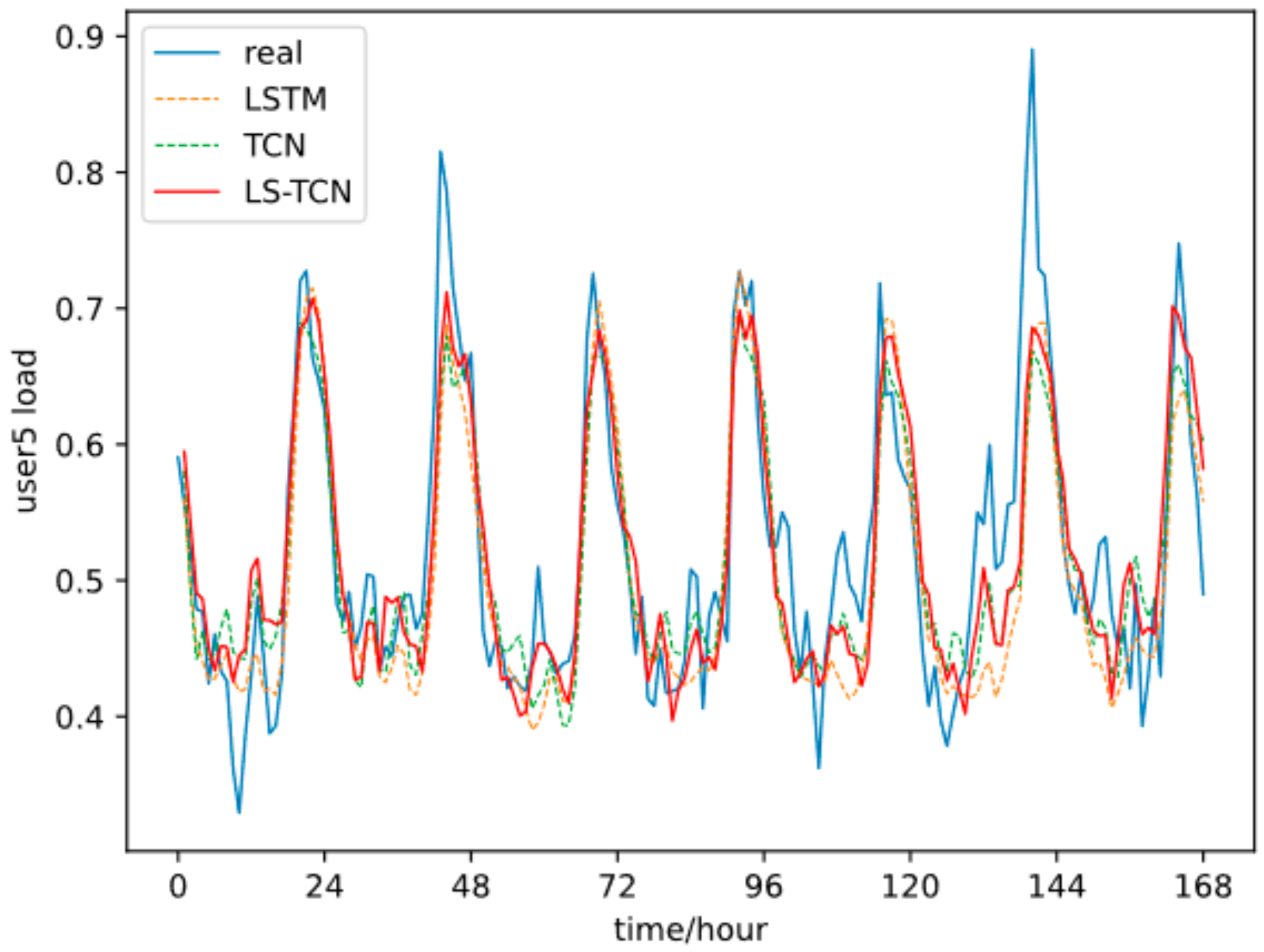
The authors qualitatively analyzed the trained LST-TCN by comparing its scores with those given by the existing translation model, such as LSTM and TCN. The qualitative analysis shows that the LST-TCN has better generalization effects and smaller prediction errors.

Our contributions are as follows:

• The paper takes the periodicity of load sequence into account;
• The paper provides an efficient model of short-term load forecasting;
• The paper provides an experimental evaluation of using the framework and comparison with other models.

2. TCN Model

The cyclic neural network splits the input data into multiple time steps and calculates them chronologically. The output of each time step is affected by the hidden state of the previous time step. Models such as RNN, LSTM, and seq2seq are usually the first to model sequence data. LSTM solved the problems of vanishing gradient and gradient explosion to a certain extent through the gate mechanism. However, it is still difficult to deal with the dependence on long series, and the serial computing mechanism leads to slow speed.

The convolutional neural network is mainly used in the field of computer vision, and its advantage lies in its powerful image feature extraction ability. According to different input data forms, the convolution operation forms of 1-D convolution, 2-D convolution, and 3-D convolution correspond to 1-D, 2-D, and 3-D tensors. Causal convolution, dilated convolution, and other technologies are also proposed to achieve a specific convolution effect.

Using a one-dimensional convolutional network to process one-dimensional load sequence data was considered. This research point is based on the time convolutional neural network for load forecasting and can take advantage of the computational parallelism of the convolutional neural network and the perceptual field of vision superior to the recurrent neural network.

The so-called time convolution neural network is a type of network based on the convolution principle, suitable for processing time-series data. For example, Aaron van den Oord et al. proposed WaveNet [21] for speech generation, and Colin Lea et al. [23] used encoder and decoder networks to realize segmentation and recognition actions based on convolution structure. In 2018, the TCN proposed by ShaojieBai et al. [22] referred to the 1-D full convolution network of WaveNet, causal convolution, and dilated convolution structure. The main difference is that the residual connection layer is added to the convolution layer; the paper organizes the effects of this network model on several sequence problems. The author claims that the effects of TCN on speech generation, machine translation and other problems, the parameters, and the training time of the model are significantly better than those of the circular neural network. The structure of each part of TCN is introduced below.

2.1. Causal Convolution

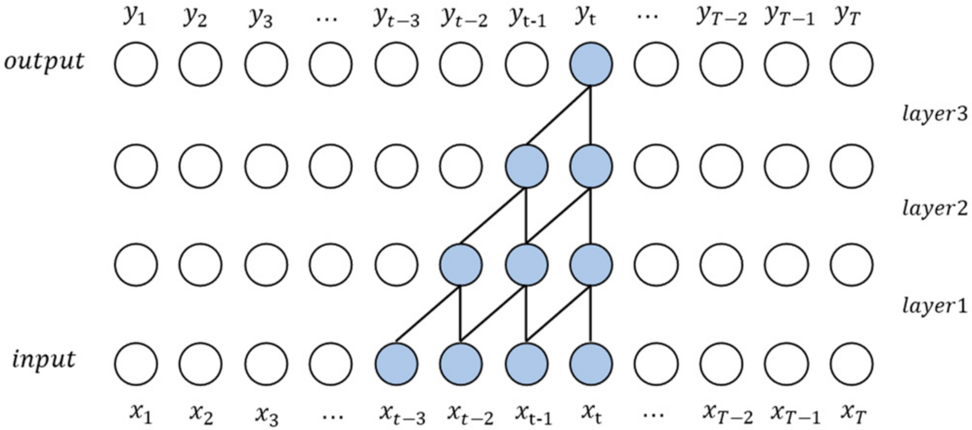
Similar to RNN, the sequence model needs to meet two principles: 1. The output length of the model is equal to the input length; 2. When processing the current time step, the leaked information of the future time step cannot be known. TCN uses a 1-D fully convolution network and padding to ensure that the length of each hidden layer is equal to that of the input layer. Causal convolution can ensure that future information does not leak from the past.

WaveNet is based on the concept of causal convolution, which inserts input sequence data $x_1,x_2,\dots ,x_T$ into the causal convolution network, and the output corresponding to each time step is $y_1,y_2,\dots ,y_T$. The structure of causal convolution ensures that the output ${\mathrm{y}}_{\mathrm{t}}$ at time t only depends on the input $x_1,x_2,\dots ,x_t$ and is not affected by $x_t+1 ,x_t+2, \dots ,x_T$ at time $t+1$ and later. Figure 2 shows the structure of multi-layer causal convolution with each layer padding on the leftmost side. The perceptual field of vision of $y_T$ is $\left(k-1\right)\times l$, where $l$ is the number of network layers, and $k$ is the size of the convolution kernel. The perceptual field of vision increases linearly by increasing the convolution kernel and deepening the network. When the length of the input sequence is long, for example, 1000, it is difficult to fully bring the input into the field of vision because the too large convolution kernel and the too deep network inevitably bring a huge number of parameters, and at the same time, the network that is too deep has problems such as gradient vanishing problem and gradient exploding problem during training.

2.2. Dilated Convolution

In order to solve the problem of insufficient perception field of view, TCN uses dilated convolution. Dilated convolution is a type of convolution idea that is proposed for the problem of image semantic segmentation, which reduces the resolution of the image and loses information; by adding holes, the perceptual field of vision can be expanded. The convolution layer introduces a dilated rate parameter, which defines the size of convolution holes. For the 1-D sequence data $x$ and filter $f$, the convolution result of the hole convolution operation $F$ and the input sequence position $s$ is defined as follows.

$$F\left(s\right)=\left(x\underset{d}{\times }f\right)\left(s\right)={\displaystyle \sum }_{i=0}^{k-1}f\left(i\right)·x_{s-d·i}$$

(1)

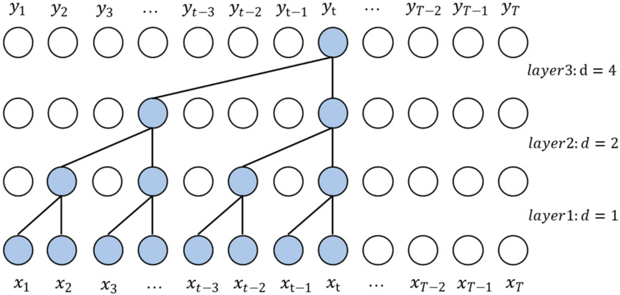
where $d$ is the hole size and $k$ is the convolution kernel size. Figure 3 shows the structure of dilated convolution. In the multi-layer hole convolution network, the hole size in each layer increases exponentially with the number of layers in the network, the hole size in the first layer $d=O\left(2^l\right)$, and the perceptual field of view = $\left(k-1\right)*d+1$. Therefore, only the network depth of $log\frac{L-1}{k-1}$ is needed to obtain the corresponding perceptual field of vision for sequences with length $L.$ For example, when the sequence length is 1024 and the convolution kernel $k$= 2, the number of network layers should be 12.

2.3. Residual Connection

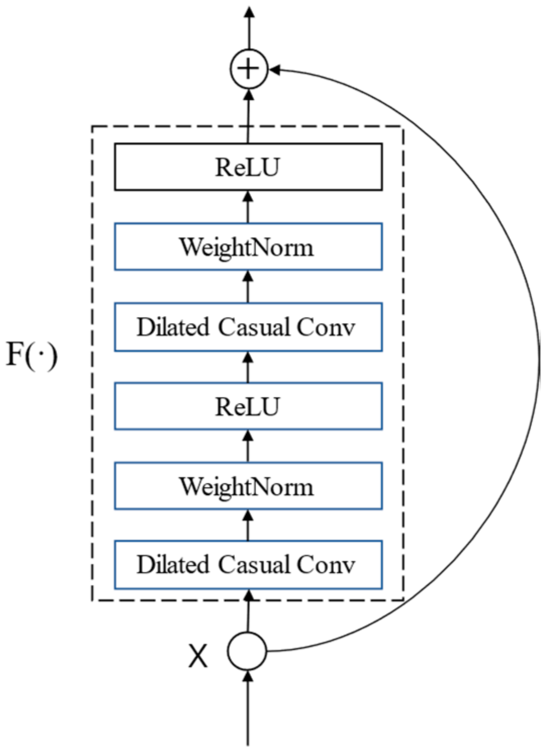
With the deepening of the network, the difficulty of training the network increases, the network degenerates, and the accuracy of the training set decreases. He et al. invented the residual connection module to solve the problem caused by the increase in the number of network layers and applied it to ResNet to train a 152-layer convolutional network, refreshing the scoring record of CNN in ImageNet. For a stacked-layer structure, when the input is $x$, the learned feature is recorded as $H\left(x\right)$, and now the residual $F\left(x\right)=H\left(x\right)-x$ is hoped to learn because residual learning is easier than direct learning of the original features. As mentioned earlier, when the historical information with the length of $2^{12}$ needs to be considered in the prediction result, a 12-layer network is needed to obtain the perception field of $2^{12}$, which is still a deep network, so residual connection is introduced for better training. The residual module is used to replace the original convolution layer in TCN. TCN residual module contains two layers of dilated residual convolution and ReLU activation function, as shown in Figure 4.

3. LST-TCN Module

The user’s electricity consumption data depend on the user’s production and lifestyle, and a certain periodicity from the load series data can be observed. For example, there is a big difference between the electricity consumption on weekends and that of the week in a weekly cycle due to vacations on weekends. The load at night is smaller than that in the daytime, and people usually use the same electrical equipment at a fixed time each day. Based on this, the proposed algorithm considers the daily periodicity of the load sequence, uses two networks to extract features from long-term data and periodic short-term data, respectively, and fuses the two features to calculate the final predicted value.

TCN receives one-dimensional sequence data and outputs a one-dimensional sequence through the dilated causal convolution and residual connection module. TCN can be used as an overall independent structure for processing sequence data to extract the sequence feature results.

Let the feature of a sample be $X$, and the dimension of $X$ is $\left(1,l\right)$, where $l$ represents the time step of the input data.

3.1. Long-Term TCN

The so-called long-term TCN is a TCN network that takes a complete $X$ as input to extract the long-term dependence of the input sequence data. There are not many skills in this part. Input $X$ directly into TCN, record the output as out, and the dimension of out as $\left(m,l\right)$. Take the last time step out $h_l=out\left[:,-1\right]$. According to the structural characteristics of TCN, vector $y_l$ has the ability and should consider the information of all time-steps of input data.

3.2. Short-Term TCN

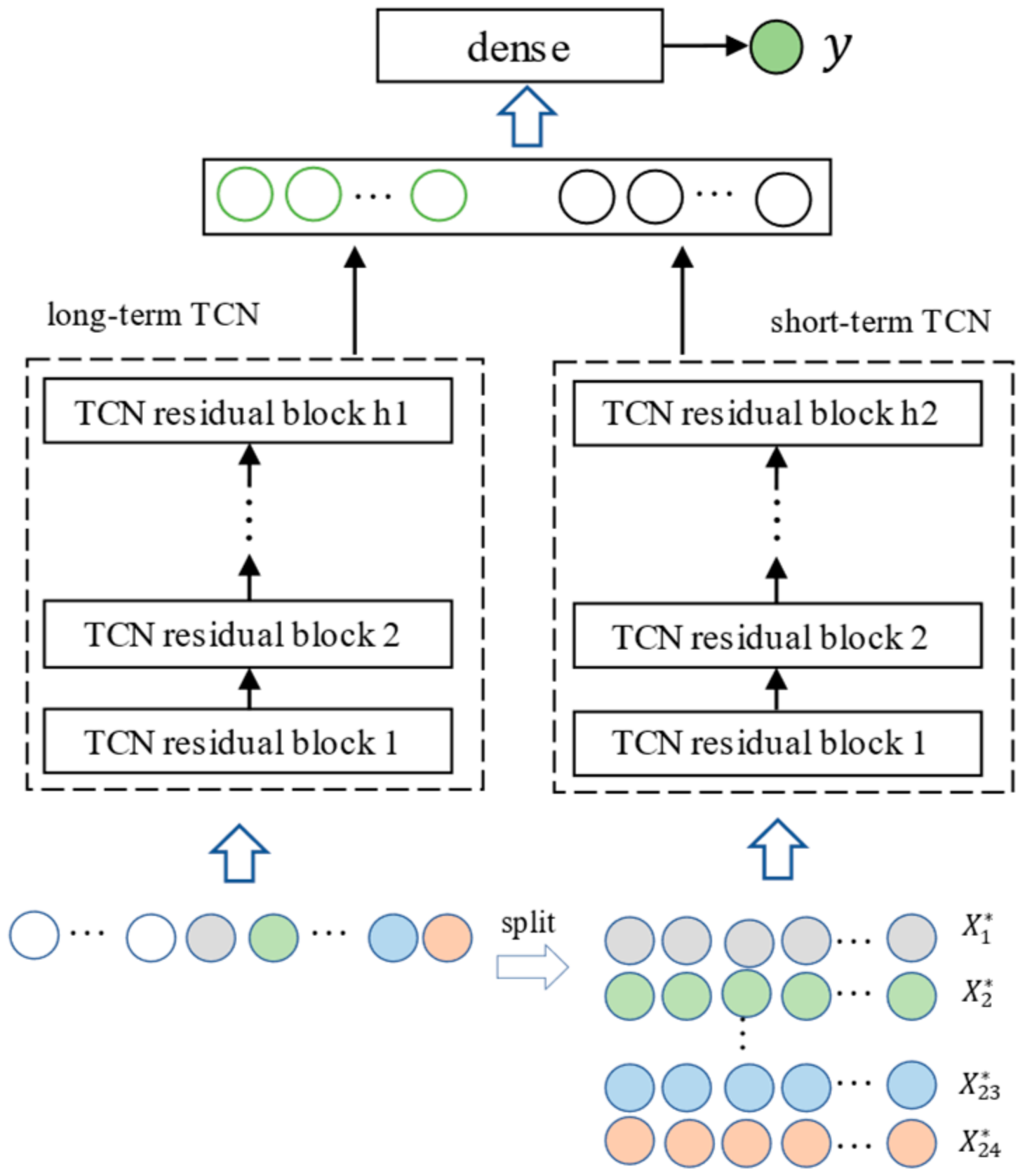
As mentioned earlier, our forecast target is the value of the sequence at a certain time step in the future, that is, the load within a certain hour in the future. Because a day is the basic cycle of people’s activities, the electricity consumption behavior of a certain hour of the day is similar to the electricity consumption behavior of that period in the past. Split the input data $X$ into 24 sub-sequences $X^{*}$, $X_i^{*}$ is composed of all the values of the ith hour in $X$, and separately consider the influence of the sub-sequences corresponding to each hour to the predicted value. Input $X_1^{*}$ to $X_{24}^{*}$ into TCN, as with long-term TCN; take out the last time step of the output layer; and obtain 24 vectors, $h_1,h_2,\dots ,h_{24}$. The dimension of $h_i$ is $\left(n,\right)$.

3.3. LST-TCN Overall Structure

The feature vectors output by the long-term TCN and the short-term TCN can be concatenated into $H=\left[h_l,h_1,h_2,\dots ,h_{24}\right]$, and the dimension of $Y$ is $\left(m+24\times n,\right)$. Input $Y$ to the fully connected layer and output the final prediction result $y$. Figure 5 shows the overall structure of LST-TCN.

4. Model Training

4.1. Loss Function

It is common to use the minimum mean square error (MSE) or the minimum absolute error (MAE) as the loss function in the training of the regression model. MSE formula

$$L_{MSE}=\frac{1}{T}{\displaystyle \sum }_{t=1}^T{\left(y_t-{\widehat{y}}_t\right)}^2$$

(2)

where $y_t$ and ${\widehat{y}}_t$ represent the actual measured value and predicted value at time t, respectively, and $T$ represents the entire predicted period.

Traditional regression neural network models can only output the expected value of the future load. This paper uses the pinball loss function instead of MSE to guide the training of the neural network model. Pinball loss function is also called quantile loss function, and its calculation formula is defined as Equation (3):

$$L_{q,t}\left(y_t,{\widehat{y}}_t^q\right)=\left\{\begin{array}{c}\left(1-q\right)\left({\widehat{y}}_t^q-y_t\right) {\widehat{y}}_t^q\ge y_t\\ q\left(y_t-{\widehat{y}}_t^q\right) {\widehat{y}}_t^q<y_t\end{array}\right.$$

(3)

where $q$ represents the target quantile, ${\widehat{y}}_t^q$ represents the qth estimated quantile of time t, and $L_{q,t}$ represents the pinball loss of the qth quantile of time t. Figure 6 shows the asymmetry of pinball loss. When the predicted quantile is higher than the true value, the penalty is multiplied by $\left(1-q\right)$, and when the predicted quantile is lower than the actual value, the penalty is multiplied by $q$.

Using pinball loss as the loss function has two advantages:

Under the guidance of pinball loss, the network model provides the target quantile value instead of the predicted expected value. By changing the quantile value, a series of quantiles can be obtained to express the uncertainty of the prediction. The entire training process is parameter-free and does not need to pre-suppose the distribution of the data.

Three aspects are usually used to evaluate the effect of probability prediction: reliability, clarity and calibration. Pinball loss is a comprehensive index that includes these three aspects so that pinball loss can guarantee the performance of the final probability prediction.

4.2. Optimizer

The optimization strategy in this article is consistent with the traditional time series prediction model, using stochastic gradient descent (SGD) or its variant Adam as the optimizer. However, Adam’s use condition is that the loss function can be differentiated everywhere, and pinball loss does not meet this requirement. Therefore, the Huber norm is applied to the loss function to make it differentiable everywhere through a small approximation. Huber Norm can be regarded as a combination of L1-norm and L2-norm,

$$H\left(y_t,{\widehat{y}}_t^q\right)=\left\{\begin{array}{c}\frac{{\left({\widehat{y}}_t^q-y_t\right)}^2}{2\delta }, 0\le \left|{\widehat{y}}_t^q-y_t\right|\le \delta \\ \left|{\widehat{y}}_t^q-y_t\right|-\frac{\delta }{2}, \left|{\widehat{y}}_t^q-y_t\right|>\delta \end{array}\right.$$

(4)

Replace ${\widehat{y}}_t^q-y_t$ in Equations (3) and (4) with $H\left(y_t,{\widehat{y}}_t^q\right)$, and the approximate pinball loss is

$$L_{q,t}\left(y_t,{\widehat{y}}_t^q\right)=\left\{\begin{array}{c}\left(1-q\right)H\left(y_t,{\widehat{y}}_t^q\right) {\widehat{y}}_t^q\ge y_t\\ qH\left(y_t,{\widehat{y}}_t^q\right) {\widehat{y}}_t^q<y_t\end{array}\right.$$

(5)

Compared with the standard pinball loss, the approximate pinball loss is different in that when the prediction error ${\widehat{y}}_t^q-y_t$ is 0. When the prediction error is greater than the threshold, the gradient is the same as the standard pinball loss, and when the prediction error is less than the threshold, the difference between the two is also very small.

4.3. Algorithm Flow

By using the sliding window method, the sequence segments of each user are captured from the load sequence, summarized into data sets, and then divided into training data sets, verification data sets, and test data sets.

Input the training set of the previous step into the model for training, retain the model parameters that have the best effect on the validation set during the training process, and finally apply the model parameters on the test set to observe the prediction effect for parameter tuning. After obtaining the optimal effect model, the data to be predicted are input into the trained model to output the prediction result.

5. Experimental Results and Analysis

This section verifies the prediction performance of the LST-TCN model proposed earlier. The real load data are selected for training and testing, and different prediction time intervals are set for experiments, respectively. Then, the prediction results of LST-TCN are compared with LSTM and TCN, and the values of pinball loss and the errors of MAPE and RMSE are compared, corresponding to 50% quantile prediction results to verify the effectiveness of LST-TCN. Mean Absolute Percentage Error (MAPE) and Root Mean Squared Error (RMSE) are defined.

$$MAPE\left(y,\widehat{y}\right)=\frac{100\%}{n}{\displaystyle \sum }_{i=1}^n|y_i-{\widehat{y}}_i|$$

(6)

$$RMSE\left(y,\widehat{y}\right)=\sqrt{\frac{1}{n}{\displaystyle \sum }_{i=1}^n{(y_i-{\widehat{y}}_i)}^2}$$

(7)

5.1. Experimental Setup

The Electricity load Diagrams 20,112,014 data were used, which contain 96-point daily load curves of 370 users from 1 January 2011 to 1 January 2015, that is, the load from 00:00 to 23:45 every 15 min. The data are a txt file, each line is a load of all users in 15 min, and the ith column represents user $i$.

Every user’s data starting from 1 January 2012 are valid. The data from 1 January 2012 to 31 December 2012 were selected for training, the data from 1 January 2013 to 31 January 2013 for verification, and the data from 1 February 2013 to 28 February 2013 for testing. For simplicity, the original sequence of 96-point daily data was compressed and merged into 24-point daily data.

The load data of 30 users from 370 users were selected randomly, and the data set was made for training, verification, and testing.

As Tingting Fand et al. [4] and Genkin A et al. [5] described, the non-time-series machine learning algorithms or non-neural network methods are difficult to real-time forecast the rapidly changing data and achieve reasonable dimension reduction compression with complex characteristics and fast dynamic changes. Additionally, the CNN methods are used to cascade the shallower and deeper feature from four different scales, fully mining the potential relationship between continuous and discontinuous data in feature graph, which is not suitable for time series forecasting.

Therefore, in our paper, LSTM and TCN were used as comparison algorithms to train and test together with LST-TCN. The hyperparameters of each model, including the number of network layers and the number of hidden layer nodes, are shown in

Table 1. Model hyperparameter settings.

Model	Parameter
LST-TCN	Long-term TCN convolutional layer: 10 Long-term TCN convolution channel: 50 Short-term TCN convolutional layer: 6 Short-term TCN convolution channel: 10
TCN	convolution layer: 10 convolution channel: 50
LSTM	number of layers: 3 hidden node: 256

. The Adam optimizer was used in training, the pinball loss described above was used as the loss function, the learning rate was 1e-4, the batch size was 256, and the number of iterative training was 100 epochs. The reason that we choose the 100 epochs is that when training after more than 100 epochs, the training time increases, and the results are not so obviously increasing.

5.2. Load Forecast Results

Table 2. The overall performance of each algorithm on ld2011_2014.

	Pinball Loss			Relative Improvement (%)
	LST-TCN	TCN	LSTM	I_TCN	I_LSTM
3 h	1.2453	1.2836	1.5494	2.90	19.63
6 h	1.3330	1.3660	1.6672	2.42	20.05
12 h	1.3797	1.4156	1.7536	2.54	21.32
24 h	1.3756	1.4196	1.6660	3.10	17.43
48 h	1.4885	1.5243	1.7629	2.35	15.57

shows the average pinball loss of LST-TCN and the comparison algorithm on the ld2011_2014 test set. LST-TCN has the lowest pinball loss in the five prediction time intervals of the test set. I_TCN and I_LSTM in the table represent the pinball loss error advantages of LST-TCN compared with TCN and LSTM, respectively.

When the quantile is set to 50%, pinball loss is equivalent to mean absolute error (MAE), and the corresponding output represents the expected load value.

Table 3. MAPE error of each algorithm.

	MAPE			Relative Improvement (%)
	LST-TCN	TCN	LSTM	I_TCN	I_LSTM
3 h	8.7201	8.8491	10.3376	1.45	15.65
6 h	9.3638	9.5393	12.0621	1.84	22.37
12 h	9.6176	9.8928	12.1342	2.78	20.74
24 h	9.5415	9.8123	11.1427	2.76	14.37
48 h	10.315	10.425	12.481	1.06	17.35

and

Table 4. RMSE error of each algorithm.

	RMSE			Relative Improvement (%)
	LST-TCN	TCN	LSTM	I_TCN	I_LSTM
3 h	0.04847	0.04936	0.05999	0.81	19.22
6 h	0.05249	0.05284	0.06422	0.67	18.26
12 h	0.05437	0.05546	0.06768	1.96	19.67
24 h	0.05421	0.05597	0.06534	3.14	19.67
48 h	0.05892	0.05879	0.07027	−0.08	16.15

record the test results of the MAPE and RMSE indicators for the 50% quantile, respectively. The result shows that LST-TCN is better than the comparison model in both indicators. Especially when the prediction is in 12 h or 24 h, our methods can have a greater improvement compared to the TCN and LSTM. In the 3 h and 6 h period prediction, our method also has an improvement compared to LSTM, but little improvement compared to the TCN, which means that the TCN method has an improvement compared to the LSTM in a shorter time period prediction.

Figure 7 shows the comparison between the predicted value of each model and the actual value of user 5.

Experiments show that the generalization effect of LST-TCN is better than LSTM and TCN. The LST-TCN can help to catch more detailed information when the load curve is changing. Therefore LST-TCN predicts more accuracy in the changing part and peak of the load curve. The model trained by one user’s data was used to predict its performance on other users’ data and to compare the generalization ability of the model.

Table 5. Generalization MAPE error of each algorithm.

Users of the Training Model /Predicted Users	Predicted User2	Predicted User4	Predicted User5
	LSTM/TCN/LS-TCN	LSTM/TCN/LS-TCN	LSTM/TCN/LS-TCN
Training User2	6.33/5.66/5.58	19.36/13.17/15.17	15.52/8.49/8.44
Training User4	7.92/5.99/5.47	13.45/12.29/12.19	12.90/9.22/8.65
Training User5	7.99/7.02/6.27	15.03/13.68/13.68	8.42/8.31/8.06

shows the MAPE values of the predicted results and actual values of the three models.

In this section, LST-TCN, a forecasting model based on TCN, was tested on day-ahead load forecasting. LST-TCN achieved a lower prediction error than the comparison model on some selected samples.

When we looked at the tables, the rows showed that we were training with a special user and predicting some other user. In row 1, user2 was used for training, and user2, user4, and user5 were for training; the results showed that our method has a lower MAPE, in addition to row 2 and row 3. The results showed that the generalization ability of our method is better than LSTM and TCN methods.

6. Conclusions

Day-ahead load forecasting can provide strategic support for electricity sales companies. Accurate load forecasting can be very important for decision makers in orderly electricity regulation and generation planning.

The existing TCN model has better prediction performance; the model’s parameters and the training time are significantly better than those of circular neural networks in speech generation, machine translation, and other problems. However, its power prediction can be improved to adapt to the power characteristics of the data.

In this paper, a neural network model called the LST-TCN model was proposed for short-term load forecasting. The proposed algorithm considers the daily periodicity of the load sequence, uses two networks to extract features from long-term data and periodic short-term data, respectively, and fuses the two features to calculate the final predicted value. The LST-TCN model often achieves a lower prediction error than the ones reported by other models on some selected samples.

Furthermore, the lack of rules for hyperparameter selection is the shortcoming of this model, and it is also one of the future research directions. Methods such as meta-heuristic algorithms can be considered for optimization. Extending LST-TCN to support more situations is also a direction for future work.

In conclusion, LST-TCN is a great choice for short-term electricity forecasting and power trading companies, and decision makers can benefit from the model.