Model Predictive Voltage Control of Uninterruptible Power Supply Based on Extended-State Observer

Abstract

Finite-set model predictive controls have been widely used in inverter control because of the flexible target control and no need of a modulation unit. However, the mismatching of prediction model parameters produces prediction errors, resulting in a significant decline in the performance of finite-set model predictive controls. Aiming at the problem of model parameter mismatch, an extended-state observer was proposed to accurately estimate the disturbance of the system in this paper, and the obtained disturbance value was added to a finite-set model predictive control controller to compensate for the prediction error and achieve parameter robustness. By constructing a prediction model of the inverter output voltage in αβ coordinates, all the possible output voltage values were predicted by using different voltage vectors and system measurement values. A set of voltage vectors that minimized the cost function was selected, and its corresponding switching state was applied to the inverter in the next sampling period to achieve control of the output voltage quality. Both the simulation and experimental results showed that the finite-set model predictive voltage control method based on the extended-state observer can estimate the total disturbance quickly and accurately, suppress the influence of capacitance parameter disturbance, and improve the control effect of an inverter.

1. Introduction

UPS (uninterrupted power supply) is a kind of power supply equipment that converts DC power into AC power with an inverter. It is usually used in many fields, such as computing, military, medical, and aviation fields, etc., and it provides reliable and high-quality power for key loads to ensure the normal operation of loads. A three-phase UPS system consists of a power supply, a battery pack, a rectifier, an inverter, and an LC filter. According to its topology, a UPS can be divided into online UPS, line-interactive UPS, and offline UPS [1]. The control of the inverter plays a very important role in the performance of a UPS. A UPS control system not only requires sinusoidal output voltage to have a constant amplitude and frequency showing low harmonic distortion, but also must have a fast dynamic response to load change.

In order to enable a UPS system to provide stable and high-quality voltage, researchers have conducted much research on inverter control strategies and have proposed a series of methods, including autodisturbance rejection control [2], PR control [3], adaptive control [4], and model predictive control (MPC) [5]. Because model predictive control can fully consider the constraints and nonlinear characteristics of a system in the control process and has a fast dynamic response and good steady-state characteristics, it has been studied and applied in various fields, such as energy storage converters [6], grid-connected inverters [7], and permanent magnet synchronous motors [8]. MPC uses a system model to predict the future behavior of variables in a sampling period and uses cost function as a tool to select the optimal behavior of output variables. In order to simplify MPC, a mathematical model is connected with a limited number of switching states to optimize the system. All the possible switching states are evaluated online in this optimization method, and then the defined cost function is minimized, which is called finite-set model predictive control (FCS-MPC). Moreover, different prediction steps have different optimization effects on the system [9]. The increase in the prediction step length and the inverter level state leads to an increase in the calculation amount. Therefore, methods of fast optimization to reduce the calculation cost have been extensively studied. In [10], a reference voltage vector was obtained using a deadbeat control principle, and the sector of the reference voltage vector was judged to reduce the evaluation of the voltage vector in the cost function, but the action delay caused by plenty of calculation was not considered. The authors of [11] sorted multiple control variables in a mathematical model and then predicted and evaluated them one-by-one to reduce the amount of calculation of the multivariable control, but it complicated the algorithm.

Using finite-set model predictive control to realize inverter control requires an accurate predictive model. However, the LC filter is affected by internal and external factors in the operation process, resulting in the mismatch of the parameters of the prediction model of inductance and capacitance. The mismatch of the parameters of the prediction model produces prediction errors and affects the prediction accuracy of the prediction model. In order to solve the problem of parameter mismatch, scholars have conducted extensive research. In the literature, [12] used measured information to calculate the actual parameters to modify a prediction model, eliminate the influence of parameter mismatch, and improve the robustness of predictive control, but it was easily affected by noise in the calculation process. The authors of [13] used a disturbance observer to reduce the influence of inductance parameter mismatch and high-frequency disturbance on the performance of a model, but the influence of disturbance caused by resistance parameter mismatch on the performance of the model still existed. In [14], the authors combined an extended-state observer with predictive control to reduce the influences of parameter uncertainty and unknown disturbance and to improve the control performance. However, most of the above studies only focus on L-type filters.

In [15], capacitance and inductance were treated separately, and the filter capacitance parameters in an LC filter were accurately predicted using the least-squares method to eliminate the influence of capacitance mismatch on output voltage. The authors of [16] adopted a continuous-set model predictive control strategy to control an inverter and proposed a robust disturbance observer to solve the parameter uncertainty, but it was difficult to add constraints directly. Some scholars have considered the influence of the LC filter on model parameter mismatch in model predictive control design. However, the problem of using an extended-state observer (ESO) to compensate for parameter mismatch has not been applied to an LC filter. Compared with the continuous-set model predictive control in [16], finite-set model predictive control does not need a PWM modulator, and the optimal switching state is directly obtained through the cost function and applied to the inverter. In order to solve the influence of parameter mismatch of a predictive model on predictive control accuracy, in this paper a finite-set model predictive control strategy is used to study the parameter mismatch of an LC filter using an extended-state observer. The main novelty is that, when the parameters of the prediction model are not mismatched, the extended-state observer can be used as a current sensor for the output current to reduce the number of sensors. In the case of parameter mismatch, the extended-state observer can compensate for the error caused by parameter mismatch to improve the accuracy of the predictive control and realize parameter robustness.

In this paper, a three-phase inverter with an output LC filter is taken as an example, and a model predictive voltage control method is designed in a static αβ coordinate system. In view of the influences of capacitor parameter mismatch and external disturbance, an extended-state observer is proposed to estimate the disturbance value and compensate for the predictive control to reduce the system error.

The contributions of this paper are summarized as follows:

• The influence of LC filter parameter mismatch on output voltage is evaluated;
• The design process of an extended-state observer is described in detail;
• Compared with traditional finite-set model predictive voltage control, the proposed finite-set model predictive voltage control method has better stability and parameter robustness;
• In the case of parameter mismatch, the robustness of the proposed finite-set model predictive control is verified through simulations and experiments, which proves the effectiveness of the method.

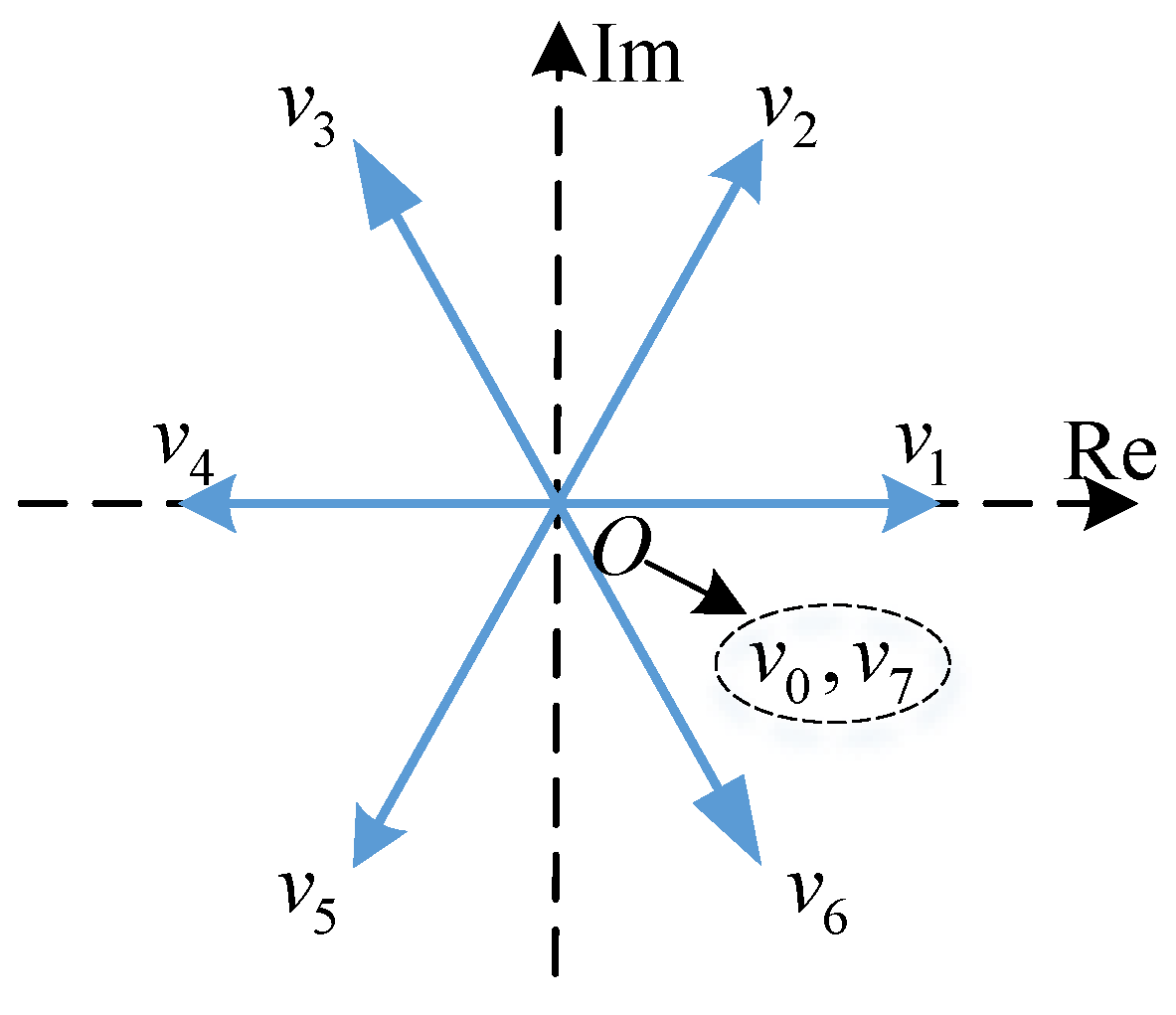
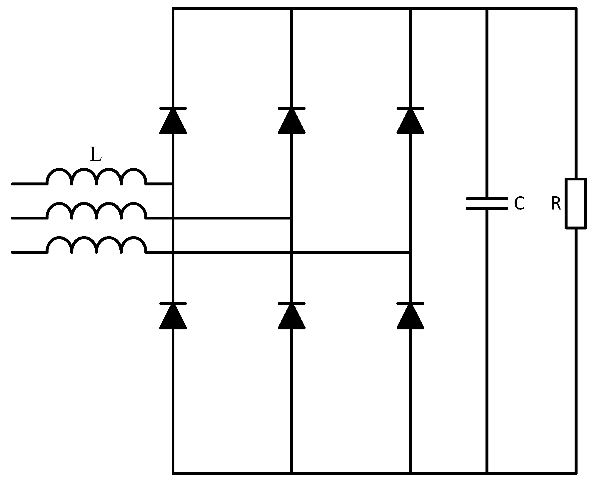
2. Traditional Model Predictive Voltage Control

2.1. System Model

The circuit of a three-phase inverter with an output LC filter is shown in Figure 1, where L is the filter inductor, C is the filter capacitor, $i_f$ is the current flowing through the filter inductor, $i_o$ is the output current, and $v_c$ is the output voltage.

According to the control signal $S_a$, $S_b$ and $S_c$ define the inverter switching states:

$$S_a=\{\begin{array}{c}1,\hspace{1em}if S_1 is ON and S_4 is OFF\\ 0,\hspace{1em}if S_1 is OFF and S_4 is ON\end{array}$$

(1)

$$S_b=\{\begin{array}{c}1,\hspace{1em}if S_2 is ON and S_5 is OFF\\ 0,\hspace{1em}if S_2 is OFF and S_5 is ON\end{array}$$

(2)

$$S_c=\{\begin{array}{c}1,\hspace{1em}if S_3 is ON and S_6 is OFF\\ 0,\hspace{1em}if S_3 is OFF and S_6 is ON\end{array}$$

(3)

The switching state vector S can be expressed as:

$$S=\frac{2}{3}(S_a+e^{j\frac{2\pi }{3}}{S}_b+e^{j\frac{4\pi }{3}}{S}_c)$$

(4)

The space vector sum of the inverter output voltage is defined as:

$$v_i=\frac{2}{3}(V_{aN}+e^{j\frac{2\pi }{3}}{V}_{bN}+e^{j\frac{4\pi }{3}}{V}_{cN})$$

(5)

where $V_{aN}$, $V_{bN}$, and $V_{cN}$ are the voltages of each phase of the inverter output relative to the neutral point $N$. Then, the relationship expression between the voltage vector and the switching state vector is:

$$v_i=V_{dc}S$$

(6)

where $V_{dc}$ is the fixed and known DC bus voltage.

Considering all the possible combinations of control signals $S_a$, $S_b$, and $S_c$, eight switching states and eight voltage vectors were obtained. Because $v_0=v_7$, seven different voltage vectors were generated, as shown in Figure 2 [17].

The filter inductance current $i_f$, the system output current $i_o$, and the output voltage $v_c$ can be expressed using a vector representation method [18].

A mathematical model of the LC filter was established, which consisted of two parts. One was the dynamic vector equation of the filter inductor current, and the other was the dynamic vector equation of the filter capacitor voltage.

The filtering current vector equation is expressed as:

$$L\frac{d{i}_f}{dt}=v_i-v_c$$

(7)

The filter capacitor voltage dynamic vector equation can be expressed as:

$$C\frac{d{v}_c}{dt}=i_f-i_o$$

(8)

The two equations can be rewritten as a state–space system:

$$\frac{dx}{dt}=Ax+B{v}_i+D{i}_o$$

(9)

where $x=\left[\begin{array}{c}{i}_f\\ v_c\end{array}\right]$; $A=\left[\begin{array}{cc}0& -1/L\\ 1/C& 0\end{array}\right]$; $B=\left[\begin{array}{c}1/L\\ 0\end{array}\right]$; and $D=\left[\begin{array}{c}0\\ -1/C\end{array}\right]$.

The output of the system is the output voltage $v_c$ shown in the following expression:

$$v_c=\left[\begin{array}{cc}0& 1\end{array}\right]x$$

(10)

For a sampling time $T_s$, zero-order hold (ZOH) discretization (12) was used to obtain the prediction of the system’s behavior as follows:

$$x\left(k+1\right)=A_{p}x\left(k\right)+B_p{v}_i\left(k\right)+D_p{i}_o\left(k\right)$$

(11)

where $A_p=e^{A{T}_s}$; $B_p={\int }_0^{T_s}{e}^{A\tau }Bd\tau$; and $D_p={\int }_0^{T_s}{e}^{A\tau }Dd\tau$.

In order to predict the output voltage $v_c$ at time k + 1, it is necessary to know the output current $i_o$ and to measure the capacitor voltage $v_c$ and the inductor current $i_f$ at time k. However, the load of a UPS is usually unknown, so the output current $i_o$ is not measurable. The estimated value of load current can be calculated using the filter current and output voltage. It can be seen from Equation (8) that the formula is:

$$i_o\left(k-1\right)=i_L\left(k-1\right)-\frac{C}{T_s}\left(v_c\left(k\right)-v_c\left(k-1\right)\right)$$

(12)

For sufficiently small sampling times $T_s$, it can be supposed that the output load does not change considerably in one sampling interval, and in that case, it can be assumed that $i_o\left(k-1\right)=i_o\left(k\right)$.

Figure 3 shows a block diagram of traditional finite set model predictive voltage control.

2.2. Cost Function

The purpose of the cost function was to select a set of optimal switching states from seven different predicted output voltages for the inverter in the next sampling period to minimize the difference between the predicted output voltage and the reference voltage at k + 1. Therefore, the cost function g can be defined as:

$$\mathrm{g}={\left|v_{c\alpha }^{*}\left(k+1\right)-v_{c\alpha }\left(k+1\right)\right|}^2+{\left|v_{c\beta }^{*}\left(k+1\right)-v_{c\beta }\left(k+1\right)\right|}^2$$

(13)

where $v_{c\alpha }^{*}\left(k+1\right)$ and $v_{c\beta }^{*}\left(k+1\right)$ are the reference voltages at the k + 1 time on the α-axis and β-axis in the stationary rotating coordinate system, respectively; and $v_{c\alpha }\left(k+1\right)$ and $v_{c\beta }\left(k+1\right)$ are the predicted output voltage values for the α and β axes, respectively.

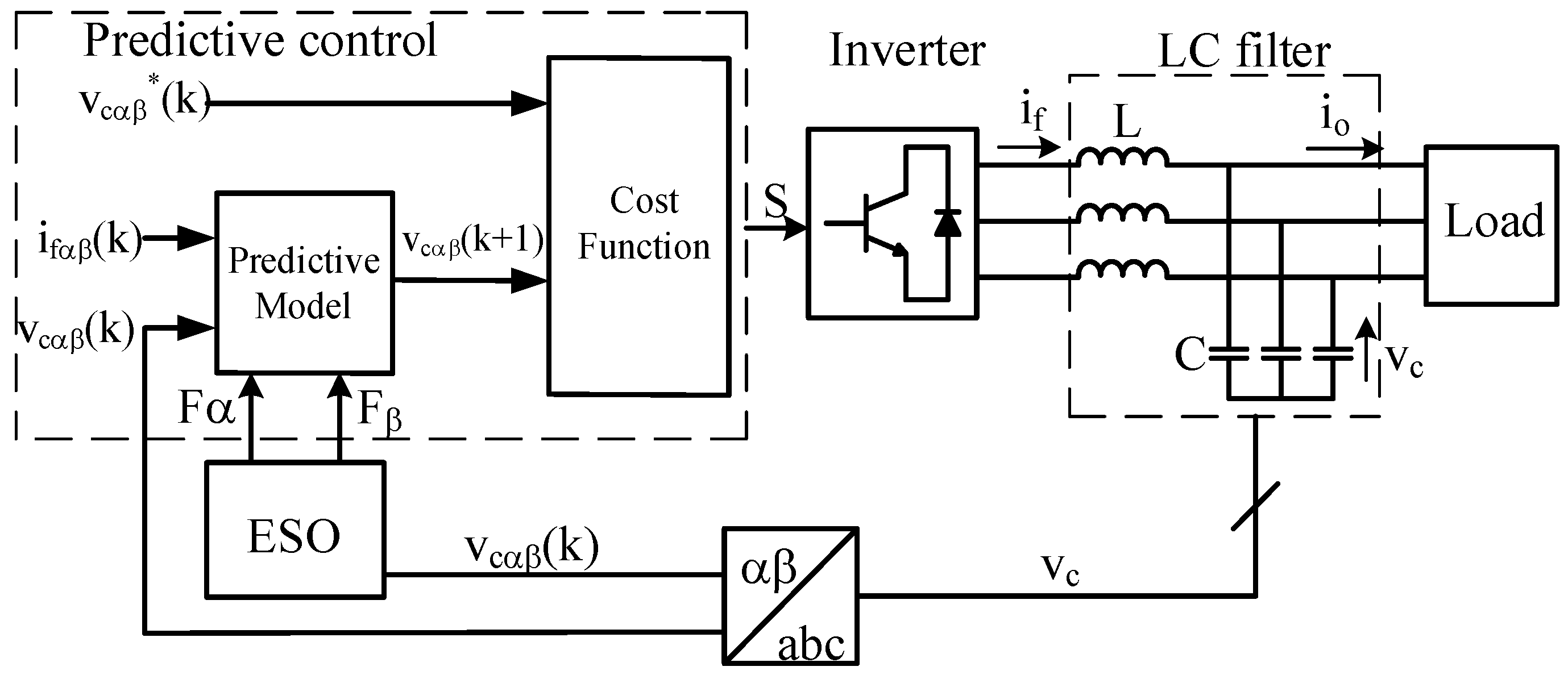
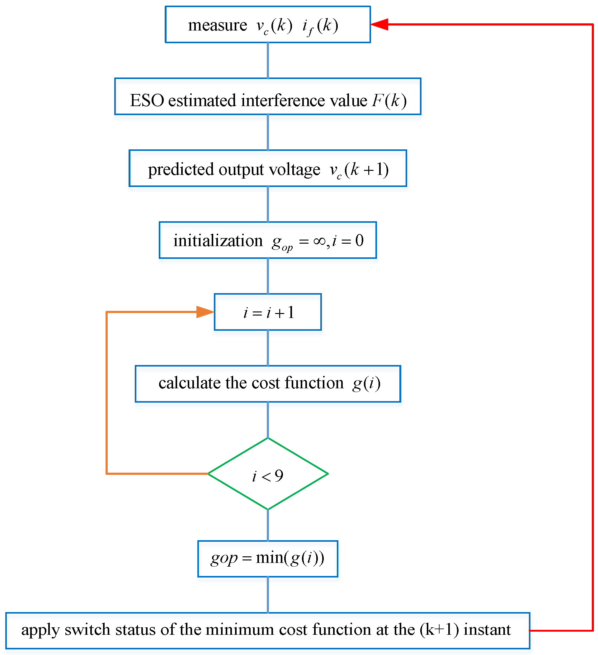
3. Model Predictive Voltage Control Based on ESO

In a traditional FCS-MPC, the disturbance caused by the mismatch of system parameters makes the predicted value deviate from the expected predicted value, which affects the control of the output voltage with a model predictive control strategy and increases the voltage harmonic. In order to overcome parameter-mismatch-induced disturbance, an ESO was used to estimate the disturbance and compensate for the estimated value in the prediction model.

3.1. Impact Analysis of Parameter Mismatch on Output Voltage

To analyze the influence of the capacitance parameter value between the model and the actual value on the output voltage, it was assumed that the capacitance in the model was $C_0$, the actual capacitance was $C_1$, and the load was R. The voltage vector equation of the filter capacitor is rewritten as:

$$\mathrm{C}\frac{d{v}_c}{dt}=i_f-\frac{v_c}{R}$$

(14)

Formulas (7) and (14) were arranged, and the Laplace transform was performed to obtain the output voltage of the model capacitor:

$$v_{c1}\left(s\right)=\frac{R{v}_i\left(s\right)}{RL{C}_0{s}^2+Ls+R}$$

(15)

The output voltage of the actual capacitance is:

$$v_{c2}\left(s\right)=\frac{R{v}_i\left(s\right)}{RL{C}_1{s}^2+Ls+R}$$

(16)

The output voltage error is:

$$\Delta v_c\left(s\right)=v_{c1}\left(s\right)-v_{c2}\left(s\right)=\frac{RL{v}_i\left(s\right)s^2\left(C_0-C_1\right)}{\left(RL{C}_0{s}^2+Ls+R\right)\left(RL{C}_1{s}^2+Ls+R\right)}$$

(17)

It can be seen from Equation (17) that the voltage error was related to the inverter output voltage and the capacitance parameter error. Assuming that the output voltage of the inverter is constant, the influence of the capacitance parameter error on the output voltage is discussed. Suppose the inductance is $2.4\mathrm{mF}$, the resistance is $50\mathsf{\Omega }$, and the voltage is $520\mathrm{V}$. The variation trends of different capacitance errors are shown in the figure below.

Figure 4 shows that the voltage error gradually increased with the frequency from 1 Hz to 100 Hz, and the voltage error caused by the three actual capacitance parameters was obviously different. When the frequency was greater than 1000 Hz, the three actual capacitance parameters had almost the same effect on the voltage error.

3.2. Mathematical Model of Parameter Mismatch

In the actual operation process, the capacitance parameters are affected by the external environment, so the output voltage dynamic vector equation can be rewritten as:

$$\left(C+\Delta C\right)\frac{d{v}_c}{dt}=i_f-i_o$$

(18)

where C is the nominal value of the capacitance of the LC filter, ΔC is the variation of the capacitance, and $C+\Delta C$ is the actual capacitance of the model.

By transforming Equation (18) from a three-phase stationary abc coordinate system to a two-phase stationary αβ coordinate system, it can be expressed as:

$$\{\begin{array}{c}\left(C+\Delta C\right)\frac{d{v}_{c\alpha }}{dt}=i_{f\alpha }-i_{o\alpha }\\ \left(C+\Delta C\right)\frac{d{v}_{c\beta }}{dt}=i_{f\beta }-i_{o\beta }\end{array}$$

(19)

The equation can be rewritten to:

$$\{\begin{array}{c}\frac{d{v}_{c\alpha }}{dt}=\frac{1}{C}{i}_{f\alpha }-\frac{1}{C}{i}_{o\alpha }-\frac{\Delta C}{C}\frac{d{v}_{c\alpha }}{dt}\\ \frac{d{v}_{c\beta }}{dt}=\frac{1}{C}{i}_{f\beta }-\frac{1}{C}{i}_{o\beta }-\frac{\Delta C}{C}\frac{d{v}_{c\beta }}{dt}\end{array}$$

(20)

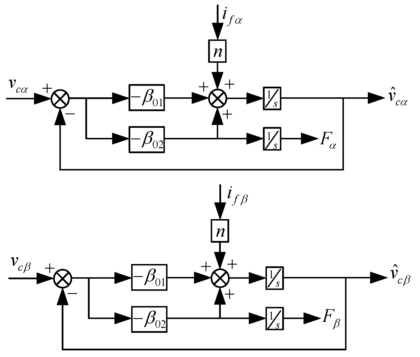
3.3. Design of Extended-State Observer

A linear ESO enables a flexible definition of the total interference. In order to simplify the analysis, the unknown part and parameter mismatch were regarded as the total disturbance, and a predictive voltage model containing disturbance F was established:

$$\{\begin{array}{c}\frac{d{v}_{c\alpha }}{dt}=\frac{1}{C}{i}_{f\alpha }+F_{\alpha }\\ \frac{d{v}_{c\beta }}{dt}=\frac{1}{C}{i}_{f\beta }+F_{\beta }\end{array}$$

(21)

Based on the filter output voltage model, two first-order linear ESOs were constructed to observe the voltage and disturbance. Taking the construction of the a-axis extended-state observer as an example, according to the ESO principle, Fα was taken as the extended variable:

$$z=\left[\begin{array}{c}{z}_1\\ z_2\end{array}\right]=\left[\begin{array}{c}{\widehat{v}}_{c\alpha }\\ {\widehat{F}}_{\alpha }\end{array}\right]$$

(22)

Extended-state observers can be constructed as:

$$\{\begin{array}{c}{e}_{\alpha }=z_1-v_{c\alpha }\\ {\dot{z}}_1=z_2+n{i}_{f\alpha }-{\beta }_{01}{e}_{\alpha }\\ {\dot{z}}_2=-{\beta }_{02}{e}_{\alpha }\end{array}$$

(23)

where $z_1$ and $z_2$ are the estimated values of the state observer, and ${\beta }_{01}$ and ${\beta }_{02}$ are the error feedback gains of the linear ESO.

${\beta }_{01}$ and ${\beta }_{02}$ are the parameters of the observer, which can affect the rapidity and stability of the observer. Therefore, selecting appropriate values can ensure the performance of the observer. Equation (23) is expressed in matrix form as:

$$\{\begin{array}{c}\dot{z}=A_{1}z+B_1{i}_{f\alpha }+D_1\left(y-\widehat{y}\right)\\ \widehat{y}=C_{1}z\end{array}$$

(24)

where $A_1=\left[\begin{array}{cc}0& 1\\ 0& 0\end{array}\right], B_1=\left[\begin{array}{c}n\\ 0\end{array}\right],C_1=\left[\begin{array}{cc}1& 0\end{array}\right], \mathrm{and} D_1=\left[\begin{array}{c}{\beta }_{01}\\ {\beta }_{02}\end{array}\right]$.

According to the above equation, the characteristic equation of an ESO can be expressed as:

$$\left|sI-\left(A_1-C_1{D}_1\right)\right|=s^2+{\beta }_{01}s+{\beta }_{02}$$

(25)

where I is the unit matrix.

According to the bandwidth method, the characteristic root must be located at $-{\omega }_0$ of the observer, and ${\beta }_{01}$ and ${\beta }_{02}$ are obtained as:

$${\beta }_{01}=2{\omega }_0,{\beta }_{02}={\omega }_0^2$$

(26)

${\omega }_0$ is the bandwidth of the extended-state observer, which plays a decisive role in the performance of the observer, so the design of ${\omega }_0$ is crucial. This paper discusses the design of ${\omega }_0$ in the z domain. The discrete-time model of Equation (23) can be described as follows:

$$\{\begin{array}{c}{e}_{\alpha }\left(k\right)={\widehat{v}}_{c\alpha }\left(k\right)-v_{c\alpha }\left(k\right)\\ {\widehat{v}}_{c\alpha }\left(k+1\right)={\widehat{v}}_{c\alpha }\left(k\right)+T_s\left({\widehat{F}}_{\alpha }\left(k\right)+n{i}_{f\alpha }\left(k\right)\right)-{\beta }_1{e}_{\alpha }\left(k\right)\\ {\widehat{F}}_{\alpha }\left(k+1\right)={\widehat{F}}_{\alpha }\left(k\right)-{\beta }_2{e}_{\alpha }\left(k\right)\end{array}$$

(27)

where ${\beta }_1=T_s{\beta }_{01}$ and ${\beta }_2=T_s{\beta }_{02}$ are the observer gains.

From the above formula, it can be derived that the transfer function of an ESO is:

$$G\left(z\right)=\frac{{\widehat{v}}_{c\alpha }\left(z\right)}{v_{c\alpha }\left(z\right)}=\frac{{\beta }_{1}z-{\beta }_1+{\beta }_2{t}_{sc}}{{\left(z-1\right)}^2+{\beta }_{1}z-{\beta }_1+{\beta }_2{t}_{sc}}$$

(28)

The characteristic equation is:

$${\left(z-1\right)}^2+{\beta }_{1}z-{\beta }_1+{\beta }_2{t}_{sc}=0$$

(29)

Considering ${\beta }_1=2{\omega }_0{t}_{sc}$ and ${\beta }_2={\omega }_0^2{t}_{sc}$ from the above formula, we can infer that the pole of $G\left(z\right)$ is:

$$z_{1,2}=1-{\omega }_0{t}_{sc}$$

(30)

${\omega }_0$ can be obtained by the following equation:

$${\omega }_0=\frac{1-z_{1,2}}{t_{sc}}$$

(31)

In general, if ${\omega }_0$ is too small or too large, it reduces the performance of the observer and affects the robustness of the system [19]. In this paper, $z_{1,2}$ was set to 0.15 [20], and when the sampling time was 33 μs, the bandwidth ${\omega }_0$ of the ESO was about 26,000.

3.4. Predictive Control Model of ESO

The extended state observer used the measured output voltage and inductance current to estimate parameter mismatch and unknown parts leading to disturbance. The estimated value was transferred to a prediction model to solve the influence of the disturbance on the performance of the control system.

According to the predicted voltage model including disturbance, the state–space model in the second part can be rewritten into the following expression:

$$\frac{dx}{dt}=Ax+B{v}_i+EF$$

(32)

where $E=\left[\begin{array}{c}0\\ 1\end{array}\right]$.

Based on a linear ESO, the total interference in a system can be compensated, and the discrete-time model can be described as:

$$x\left(k+1\right)=A_{p}x\left(k\right)+B_p{v}_i\left(k\right)+E_{p}F\left(k\right)$$

(33)

where $E_p={\int }_0^{T_s}{e}^{A\tau }Ed\tau$.

A model predictive voltage control scheme based on an ESO is shown in Figure 5.

Figure 6 shows the control diagram of the extended-state observer. It can be seen from Figure 6 that the disturbance caused by parameter mismatch could be estimated through the ESO. In Figure 7, a flow chart of a control algorithm combining an extended-state observer and a finite-set model predictive control is presented, which was used to improve parameter robustness.

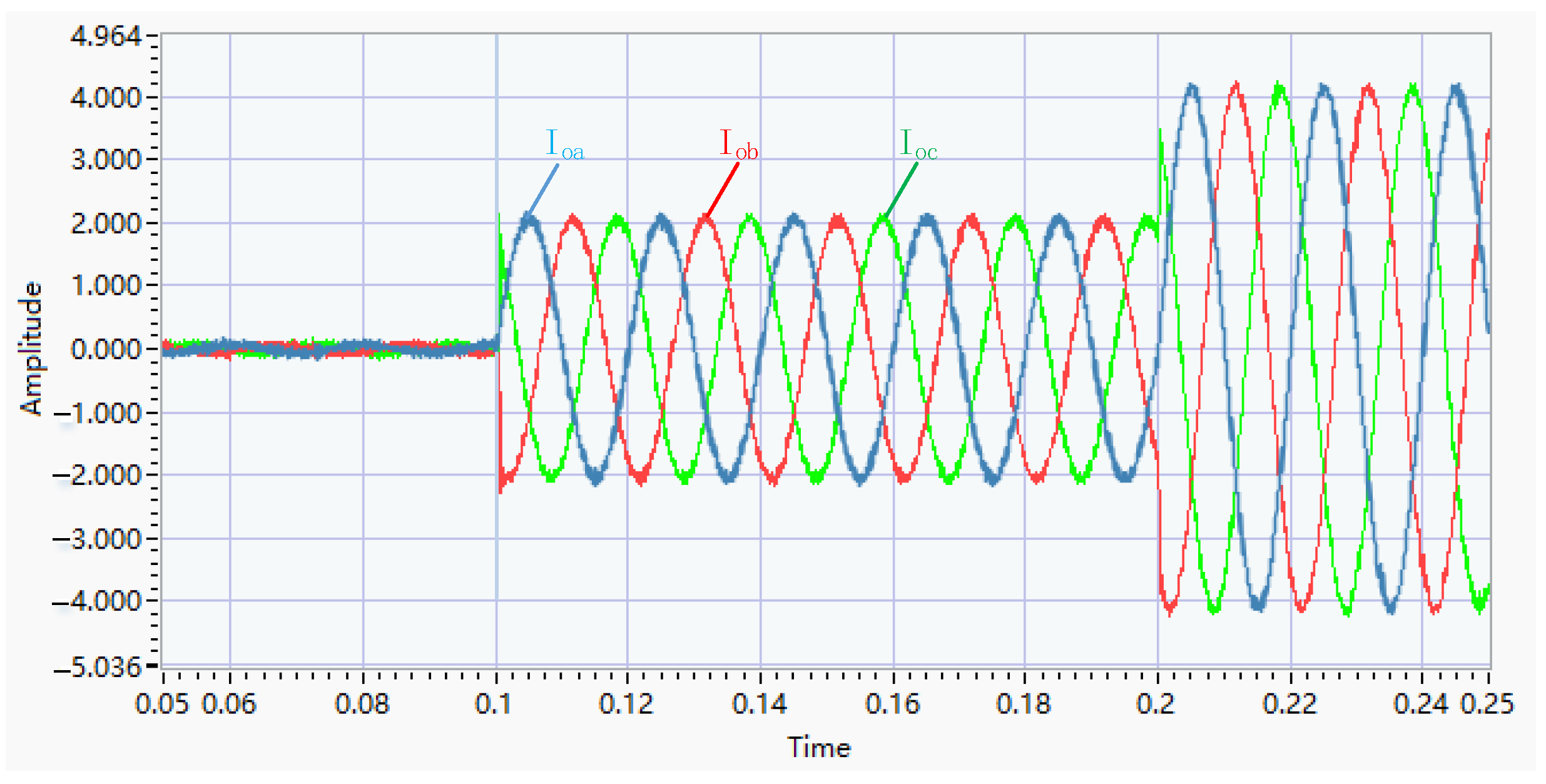
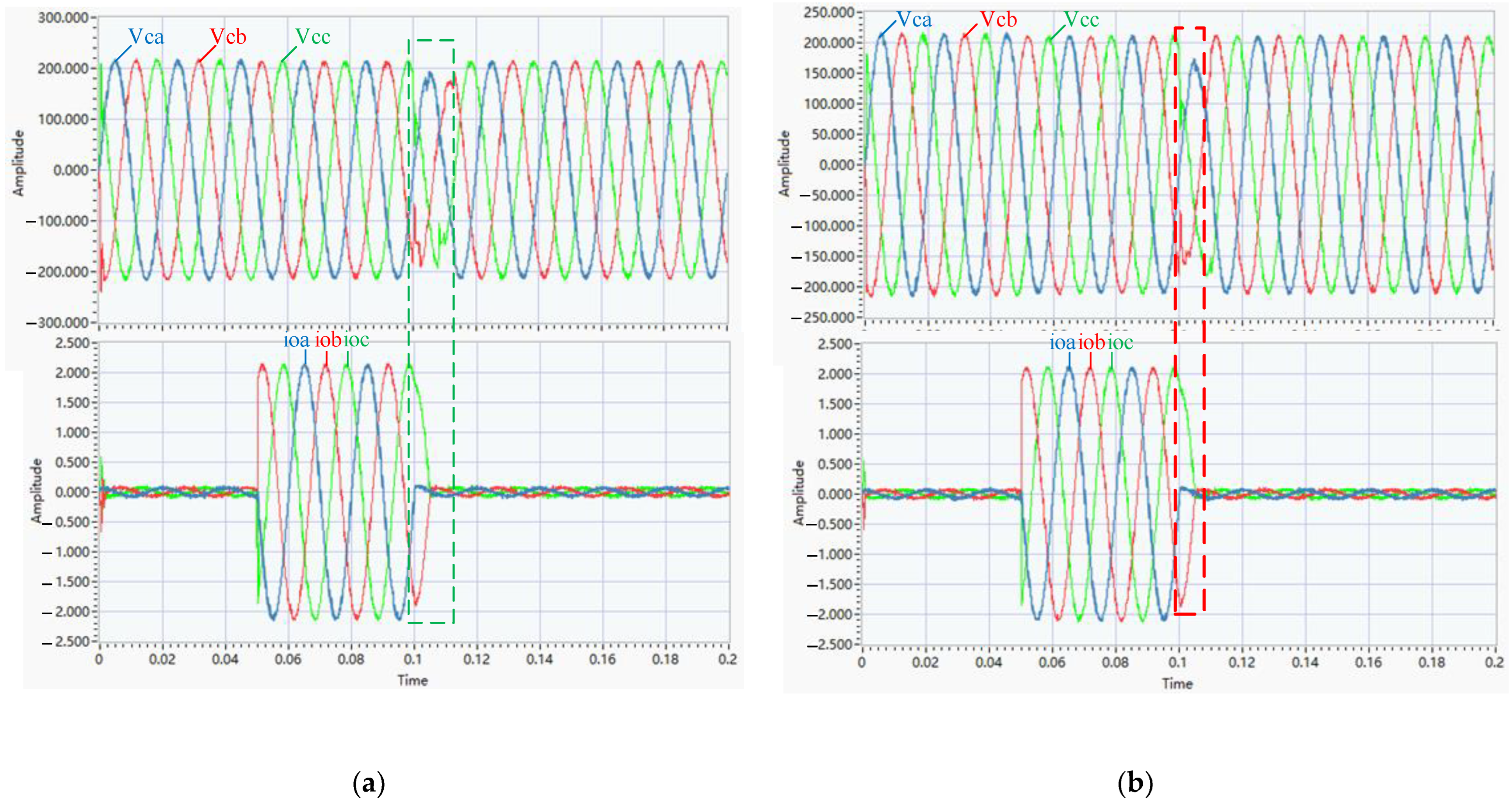
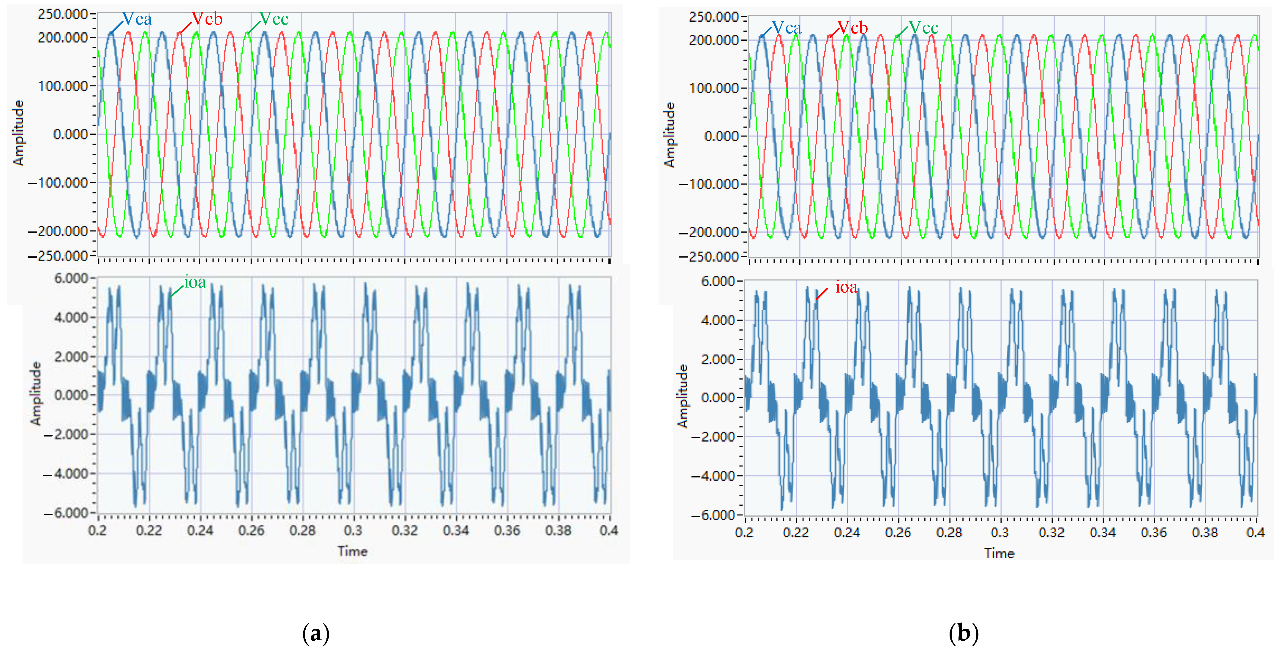
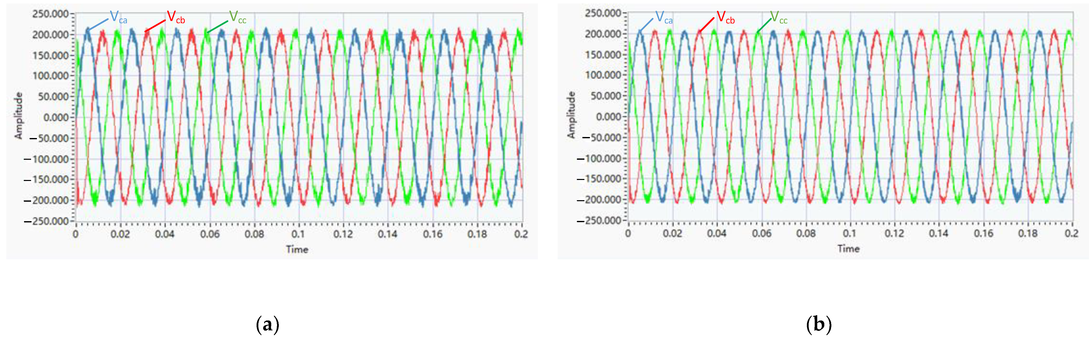
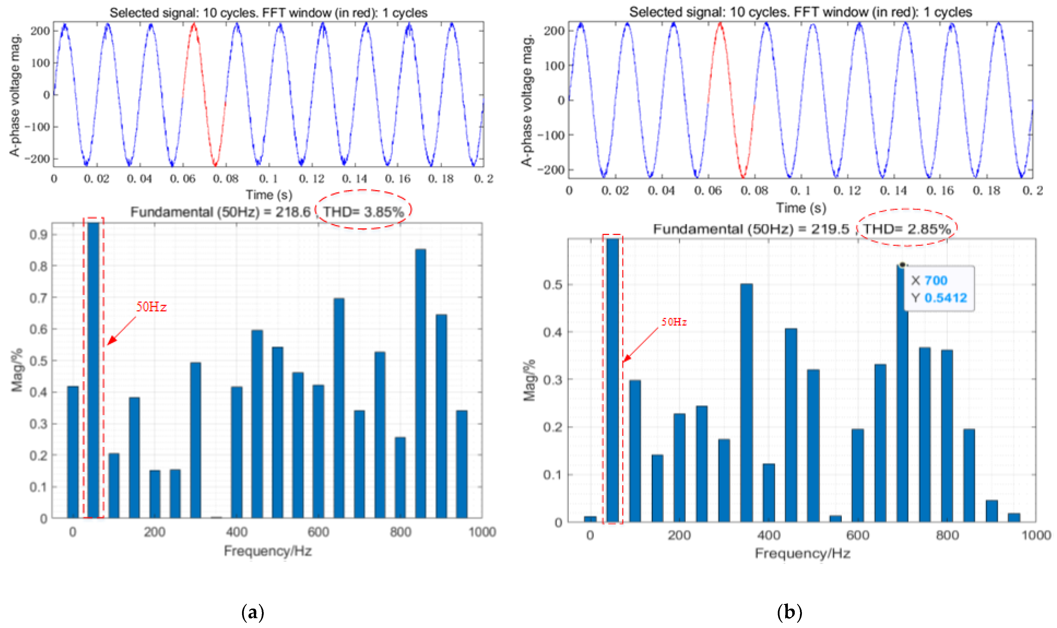
4. Simulation and Experimental Results

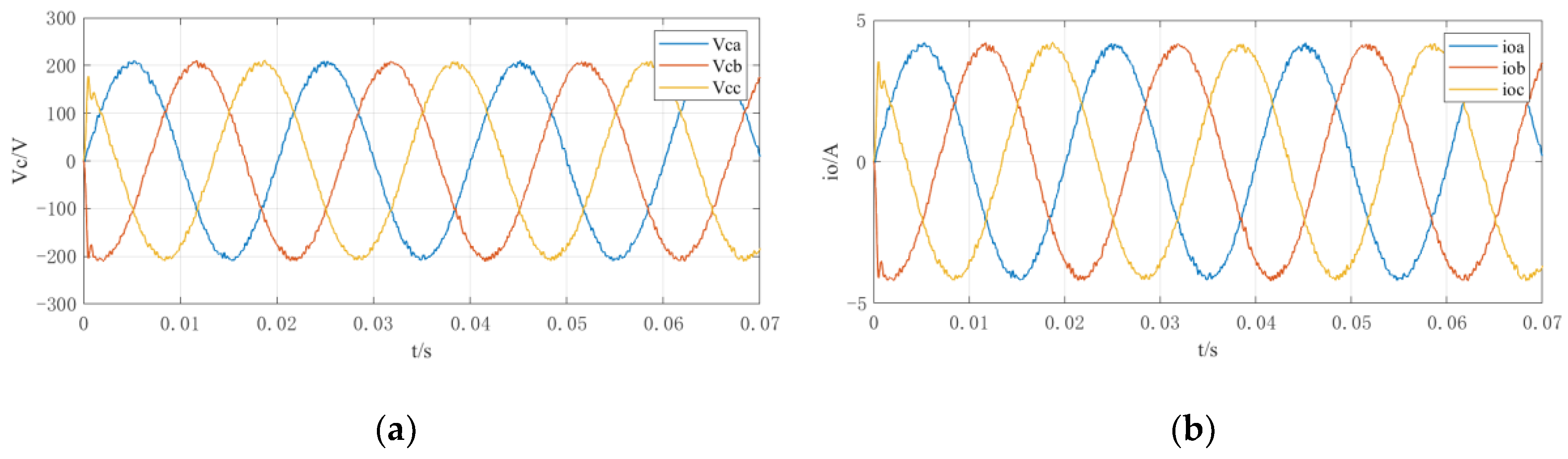
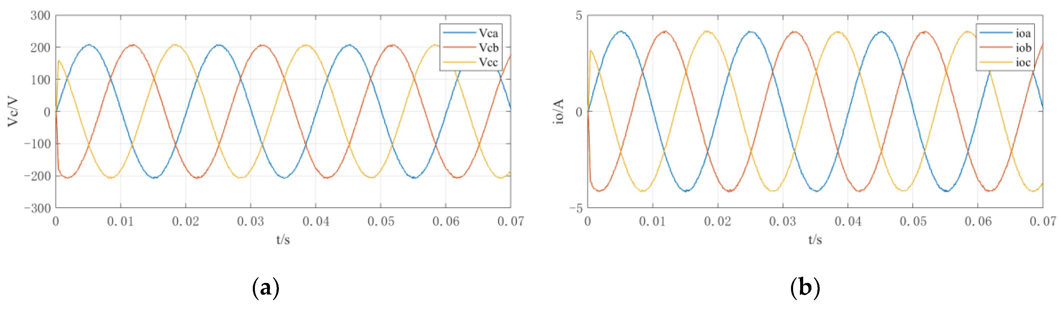
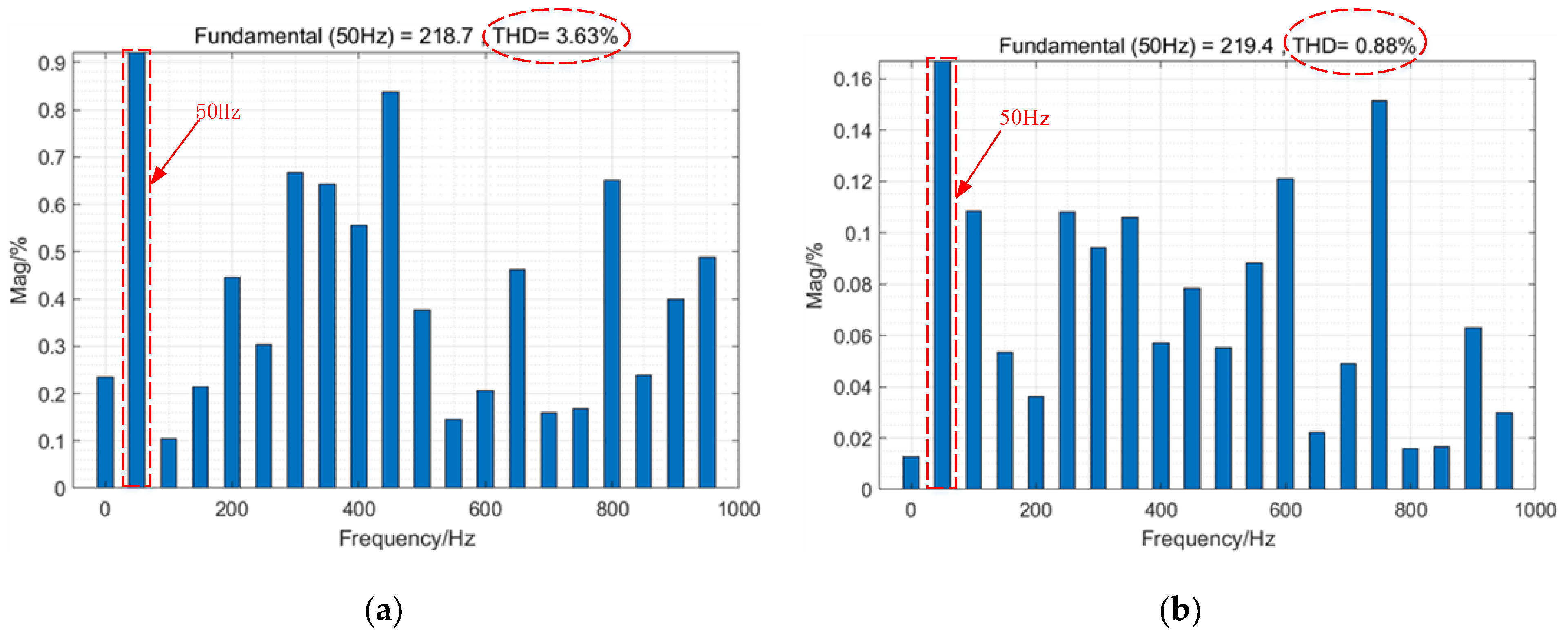
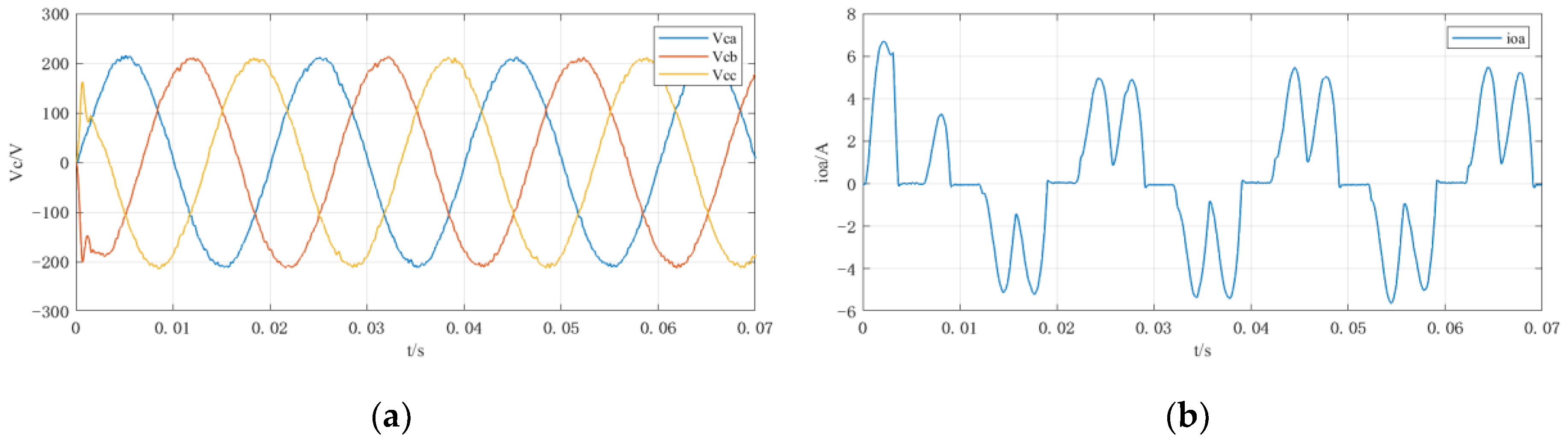
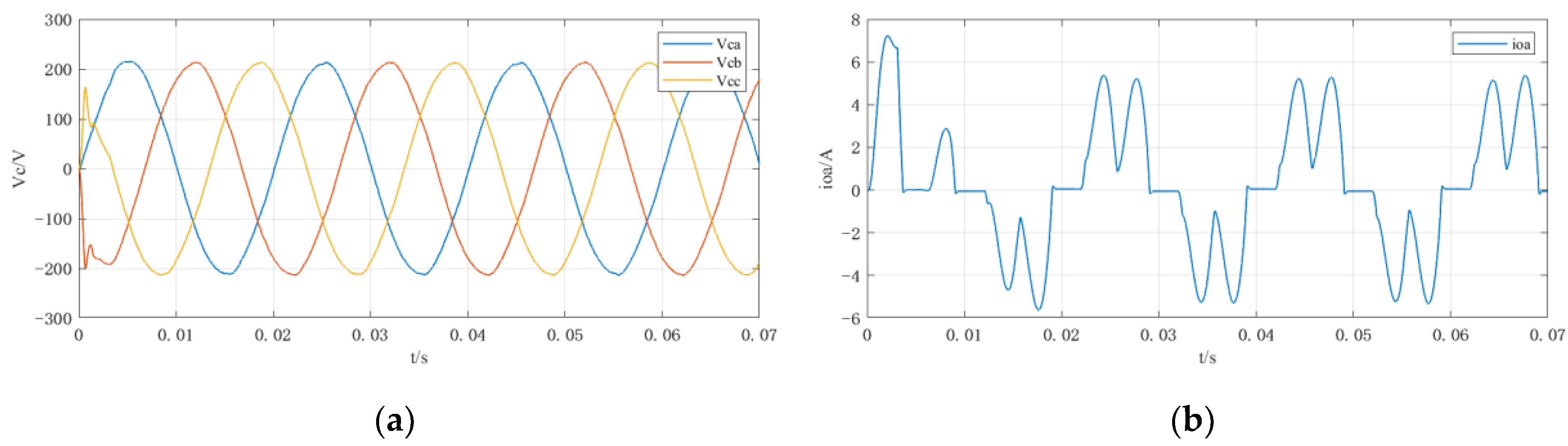
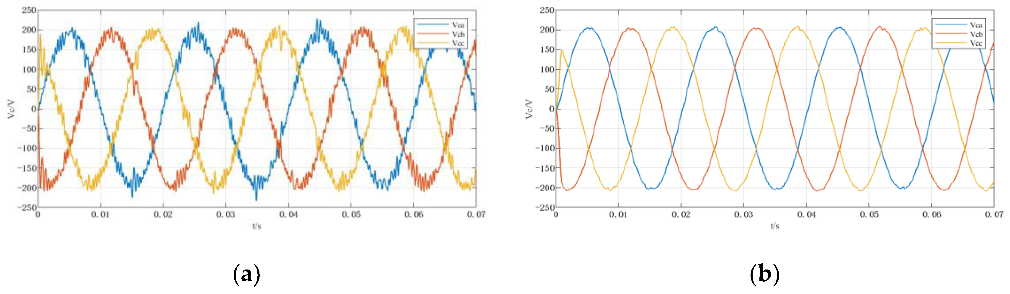
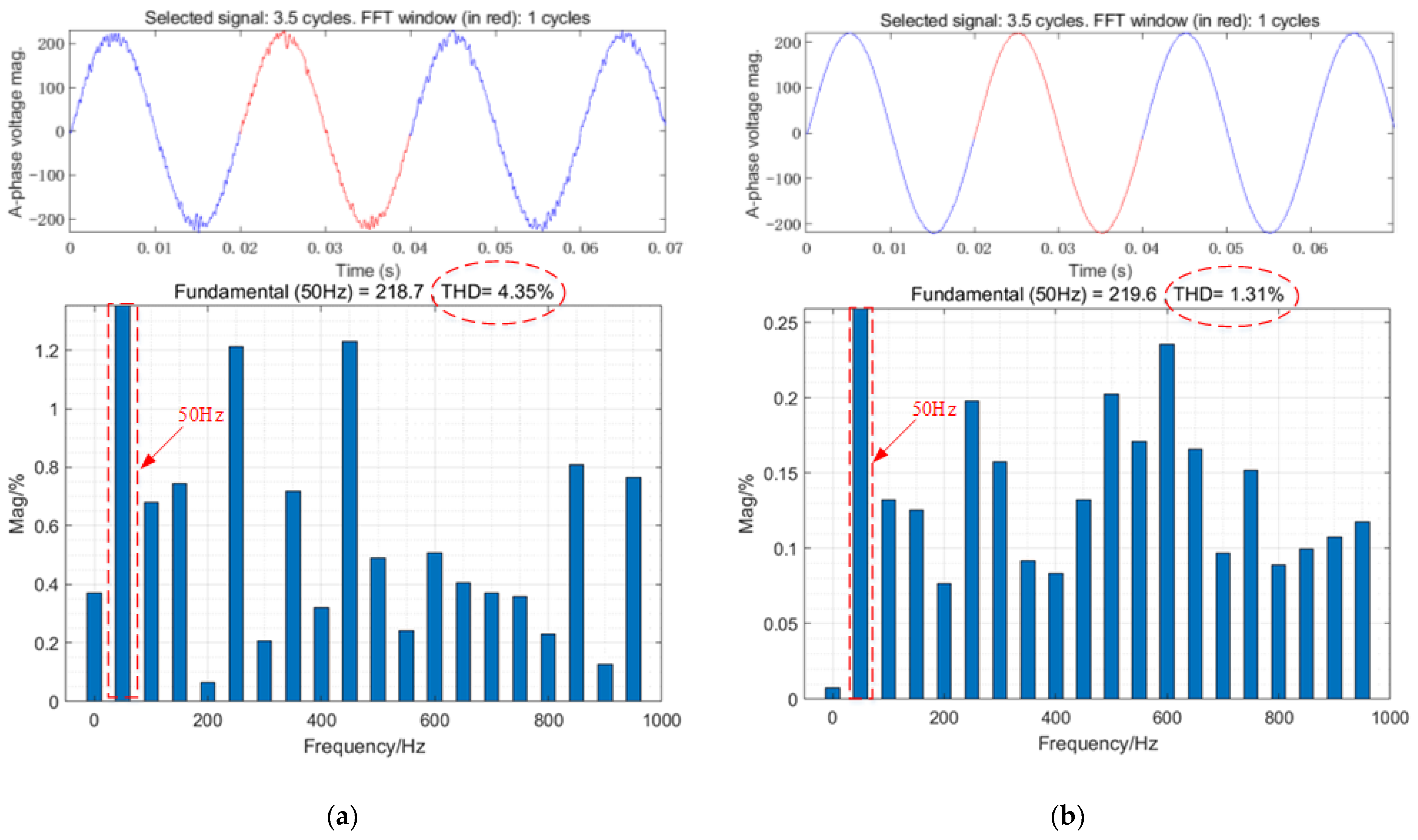
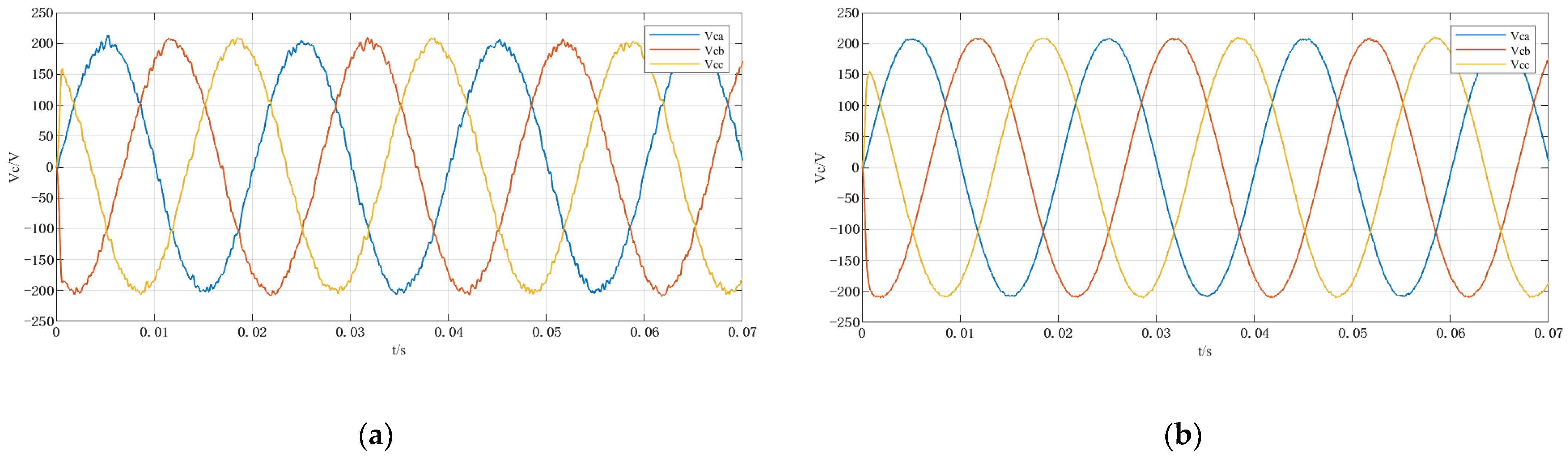
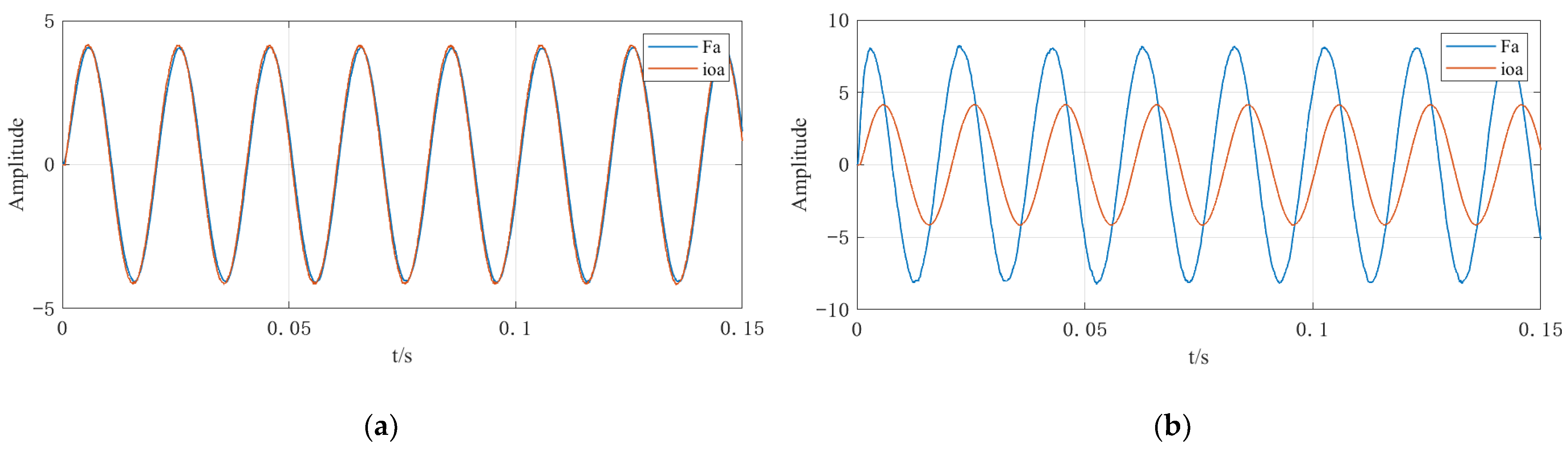
4.1. Simulation Results

In order to verify the control effect of the proposed ESO-based model predictive voltage control on the output voltage, a Matlab Simulink simulation model was built that was verified under a pure resistive load and a nonlinear load, respectively. According to the actual working conditions and load conditions of the UPS, the simulation and experimental parameters [21] are shown in

Table 1. System parameters.

Parameter	Value
$\mathrm{DC}\mathrm{link}\mathrm{voltage}{V}_{dc}$	520 V
Filter inductance L	2.4 mH
Filter capacitor C	40 μF
$\mathrm{Sampling}\mathrm{time}{T}_s$	33 μs

.

In this paper, the reference voltage amplitude was set to 220 V, and the frequency was 50 Hz. In the case of the pure resistance load, the output voltage and current waveforms of the two methods when the load power was 3 KW are discussed.

Figure 8 and Figure 9 show the comparison of the inverter output power qualities of the conventional model predictive voltage control and the model predictive voltage control based on ESO under pure resistance loads, respectively. From Figure 8, it can be seen that there were obvious harmonics in the waveforms of output voltage and current without the extended-state observer for disturbance measurement. From Figure 9, it can be seen that, when the extended-state observer was set, the output voltage and current waveforms showed smooth, sinusoidal curves during stable operation.

Figure 10 shows the harmonic spectra of the output voltage of the UPS system with two control methods. From

Table 2. Comparison of two methods under different loads.

Pure Resistor Load/W	Traditional MPC	MPC Based on ESO
	THD/%	THD/%
100	3.67	0.94
3000	3.63	0.88
30,000	2.54	0.91

and Figure 10, it can be seen that voltage control strategy with the extended-state observer had low output voltage harmonics, showing good stability.

Figure 11 shows the simulation results of verifying the dynamic performance of the control system. The system changed from no load to a 3 KW load in 0.05 s, and from a 3 KW load to no load in 0.1 s. It can be found that the system had little effect on the output voltage from no load to a load. During system unloading, the control system could control the voltage to quickly reach a stable state. The simulation results showed that the finite-set model predictive control had good dynamic performance.

In this paper, a diode bridge rectifier circuit was used to simulate a nonlinear load. Figure 12 is the schematic diagram of the nonlinear load in the simulation model. In the case of the nonlinear load, the output voltage and phase A current waveforms of the two methods are discussed when the capacitance was 100 μF, and the resistance was 100 Ω.

Figure 13 shows the output voltage and current waveforms without an extended-state observer under a nonlinear load. Figure 14 considers the output voltage and current waveforms of the extended-state observer. It can be seen that the output current had obvious distortion under the nonlinear load. The finite-set model predictive control method based on ESO was effective for output voltage control under a nonlinear load.

Table 3. Comparison of two methods under different nonlinear loads.

Resistance/Ω	Capacitance/μF	Traditional MPC	MPC Based on ESO
		THD/%	THD/%
400	100	3.40	1.36
400	2000	3.06	1.45
300	500	2.81	1.60
800	500	3.14	1.09

shows that, for the model predictive voltage control method based on ESO, when the resistance was constant, increasing the load capacitance led to increased harmonics; when the capacitance was constant and the resistance increased, the harmonics decreased.

The performance of a predictive controller depends largely on the parameters used in the predictive model, considering the influence of parameter variation on the control system. A change in the capacitance value was introduced into the prediction model, that is, the actual values were C = 20 μF and C = 150 μF.

Figure 15 shows the control effect of the UPS control system on output voltage without considering the mismatch between the capacitance model parameters and the actual values. Figure 16 shows the control effect of the UPS control system on output voltage considering the mismatch between the capacitance model parameters and the actual values. Comparing Figure 15 with Figure 16, it can be seen that the disturbance caused by parameter mismatch was not considered, resulting in a decline in the quality of the output voltage. The model predictive voltage control based on ESO had a significant inhibitory effect on the disturbance caused by parameter mismatch and improved the output voltage quality.

When the inductance parameters were mismatched and the actual inductance was $L_1=0.75L$, the suppression effects of the two control methods on the inductance mismatch were compared, as shown in Figure 17. The results show that the extended-state observer could compensate for the disturbance caused by inductance mismatch and could reduce the harmonics of the output voltage.

Figure 18 shows the output voltage waveform of parameter mismatch when the actual inductance was $L_1=0.75L$ and the actual capacitance was $C_1=2C$. The total harmonic distortion of the output voltage obtained using the traditional method was 2.62%, while the method proposed in this paper yielded 0.66%, and the difference between them was 1.96%. The results show that the proposed method could compensate well for the disturbance caused by parameter mismatch to improve the quality of the output voltage.

In Figure 19, Fa is the value of phase A, which was obtained through the following steps. First, the disturbance value obtained with the ESO was multiplied by $T_s$ and then put through Clark inverse transformation. Figure 19a shows the waveform of Fa and the actual measured current of phase A. The results show that the extended-state observer could be used as an output current sensor when the capacitance parameters of the predictive model were matched. It can be seen from Figure 19b that the waveform of Fa and the waveform of the phase A output current were different in phase and amplitude at the same time. In the case of capacitor parameter mismatch, the extended-state observer did not obtain the output current of phase A, but it did compensate for the capacitor parameter mismatch.

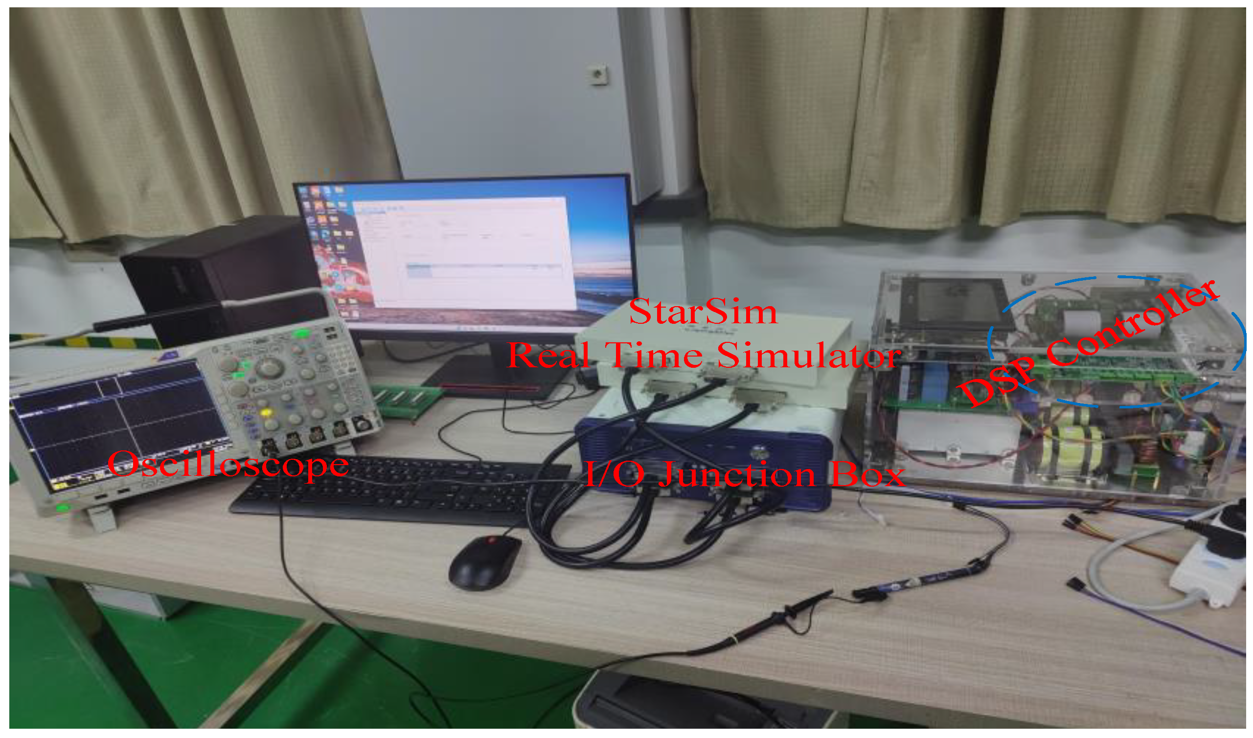
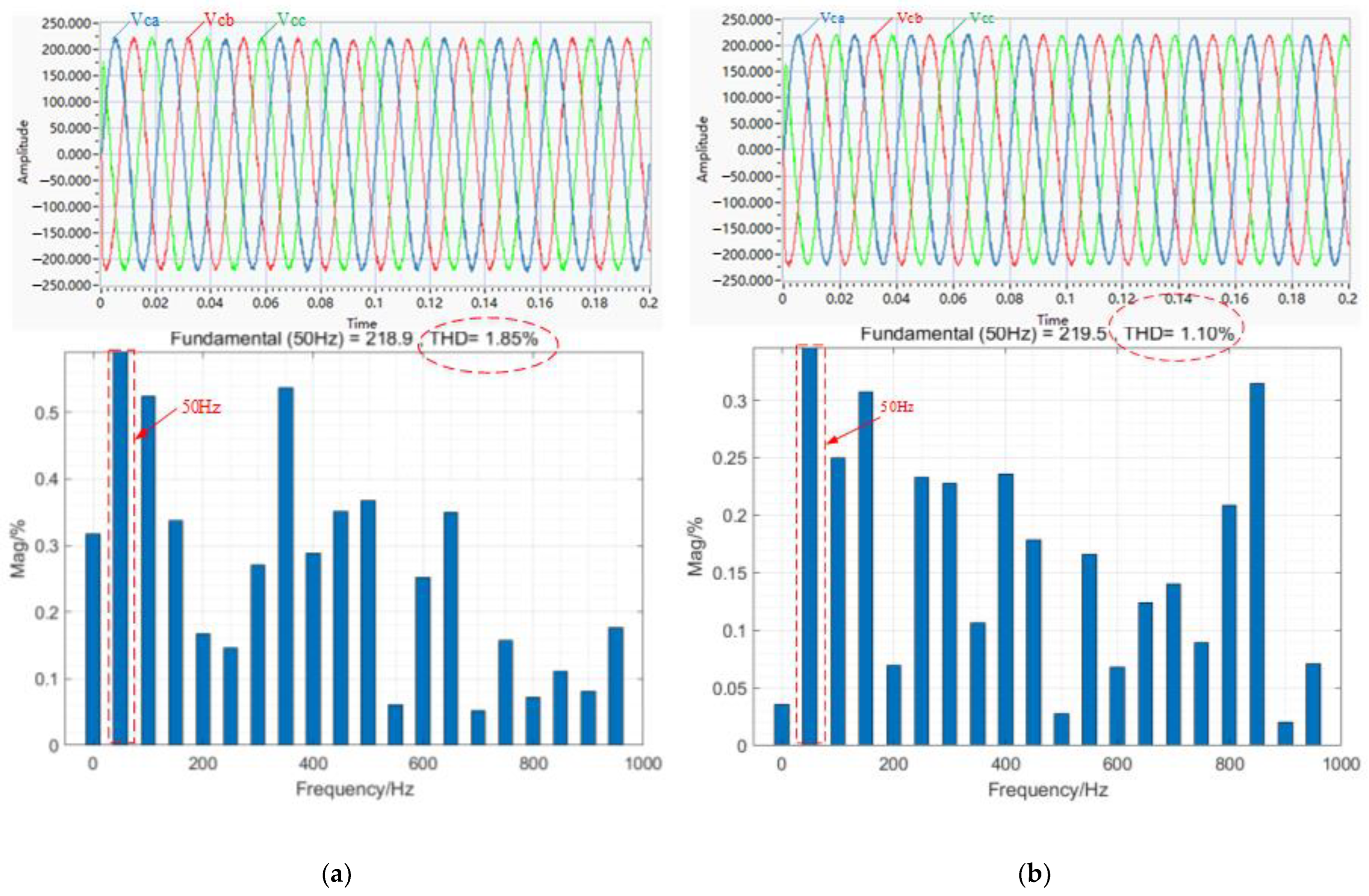
4.2. Experimental Results

Figure 20 is a diagram of the experimental equipment, which included a StarSim real-time simulator and a DSP controller; the real-time simulator and the controller were interconnected with a real, physical IO.

In order to verify the method proposed in this paper, dynamic experiments were carried out with the Yuankuan experimental platform to explore the dynamic performance and stability of the method and to compare the parameter robustness with a traditional finite-set model predictive control method. The load in the experimental tests was 3 KW.

Figure 21 shows the dynamic waveform of the output current when the load and output voltage changed.

Figure 22 shows the waveforms of the output voltage and current during the system load-switching process. The load was changed from zero to 3 KW at 0.05 s, and it was restored to zero at 0.1 s. The system was connected to the load in 0.05 s, and the voltage did not change. After 0.1 s, the system became no-load, and the output voltage presented a short adjustment process. From the experimental results, it can be observed that the dynamic performance of the method proposed in this paper was better than the traditional method for the process of system unloading.

Figure 23 shows the waveforms of the output voltage and phase A output current of the system under a nonlinear load. The experimental results show that the output voltage was sinusoidal, and the output current waveform was not sinusoidal under a nonlinear load.

When the capacitance parameters were mismatched, the actual capacitance was $C_1=0.5C$. Figure 24 shows the experimental waveforms of the output voltage. Through harmonic analysis, it was found that the output voltage THD of the traditional control method was 5.94%, and the method proposed in this paper had a THD of 3.34%, which means the quality of the output voltage was better than that of the traditional method.

Figure 25 shows the output voltage waveforms with an actual inductance of 1.8 mH, while Figure 26 shows the harmonic analysis of the phase A output voltage from 0.06 to 0.08 s, which shows that this method could also suppress the interference caused by the mismatch of inductance parameters.

Figure 27 shows the output voltage waveforms and the THD analysis of the parameter mismatch when the actual inductance was $L_1=0.75L$ and the actual capacitance was $C_1=2C$. The total harmonic distortion is shown in the figure.

5. Conclusions

In this paper, a traditional model predictive voltage control method and an ESO-based model predictive voltage control method were compared. The control performances of the two methods on the output voltage under a pure resistive load and a nonlinear load were analyzed, and the output voltage waveforms and harmonic distortion distribution when the filter capacitor parameters changed were discussed. The results showed that the proposed extended-state observer was combined with a finite-set model predictive control to realize the non-offset tracking control of a UPS system and to reduce the harmonic distortion of the output voltage. The extended-state observer could compensate for the influences of model parameter mismatch and load current and reduced the use of current sensors, improving the robustness of the control system.

References

1. Shahzad, D.; Pervaiz, S.; Zaffar, N.A.; Afridi, K.K. GaN-based high-power-density AC–DC–AC converter for single-phase transformerless online uninterruptible power supply. IEEE Trans. Power Electron. 2021, 36, 13968–13984. [Google Scholar] [CrossRef]
2. Han, Y.; He, G.; Fan, X.; Zhao, Q.; Shen, H. Design and analysis of improved ADRC controller for multiple grid-connected photovoltaic inverters. Mod. Phys. Lett. B 2018, 32, 34–36. [Google Scholar] [CrossRef]
3. Prabhakaran, P.; Krishna, S.M.; Febin, D.J.L.; Perumal, T. A novel PR controller with improved performance for single-phase UPS inverter. In Proceedings of the 2021 4th Biennial International Conference on Nascent Technologies in Engineering, NaviMumbai, India, 15–16 January 2021. [Google Scholar]
4. Li, J.; Sun, Y.; Li, X.; Xie, X.; Lin, J.; Su, M. Observer-based adaptive control for single-phase UPS inverter under nonlinear load. IEEE Trans. Trans. Electr. 2022, 8, 2785–2796. [Google Scholar] [CrossRef]
5. Caseiro, L.M.A.; Mendes, A.M.S.; Cruz, S.M.A. Cooperative and dynamically weighted model predictive control of a 3-Level uninterruptible power supply with improved performance and dynamic response. IEEE Trans. Ind. Electron. 2020, 67, 4934–4945. [Google Scholar] [CrossRef]
6. Na, Z.; Kaitao, Z.; Hui, Z.; Xi, X. Model predictive control of energy storage converter with feedback correction. In Proceedings of the 2017 Chinese Automation Congress, Jinan, China, 20–22 October 2017. [Google Scholar]
7. Qin, G.; Chen, Q.; Zhang, L. Finite control set model predictive control based on three-phase four-leg grid-connected inverters. In Proceedings of the 2020 35th Youth Academic Annual Conference of Chinese Association of Automation, Zhanjiang, China, 16–18 October 2020. [Google Scholar]
8. Chen, Z.; Qiu, J. Adjacent-vector-based model predictive control for permanent magnet synchronous motors with full model estimation. IEEE J. Emerg. Sel. Top. Power Electron. 2022. [Google Scholar] [CrossRef]
9. Cortes, P.; Rodriguez, J.; Vazquez, S.; Franquelo, L.G. Predictive control of a three-phase UPS inverter using two steps prediction horizon. In Proceedings of the IEEE International Conference on Industrial Technology, Via del Mar, Chile, 14–17 March 2010. [Google Scholar]
10. Chan, R.; Kim, K.H.; Park, J.Y.; Kwak, S.S. Simplified model predictive control with preselection technique for reduction of calculation burden in 3-Level 4-leg NPC inverter. In Proceedings of the 2020 IEEE Applied Power Electronics Conference and Exposition, New Orleans, LA, USA, 15–19 March 2020. [Google Scholar]
11. Zhang, H.; Ma, Z.; Li, Z.; Zhang, X.; Liao, Z.; Lin, G. Multivariable sequential model predictive control of LCL-type grid connected inverter. In Proceedings of the 2021 IEEE International Conference on Predictive Control of Electrical Drives and Power Electronics, Jinan, China, 20–22 November 2021. [Google Scholar]
12. Chun, H.; Jianhui, H.; Yong, L. Robust predictive current control for PMSM drives with parameter mismatch. In Proceedings of the 2021 IEEE International Conference on Predictive Control of Electrical Drives and Power Electronics, Jinan, China, 20–22 November 2021. [Google Scholar]
13. Yuan, X.; Xie, S.; Chen, J.; Zhang, S.; Zhang, C.; Lee, C.H.T. An enhanced deadbeat predictive current control of SPMSM with linear disturbance observer. IEEE J. Emerg. Sel. Top. Power Electron. 2022. [Google Scholar] [CrossRef]
14. He, C.; Hu, J.; Ran, X. Finite control set model predictive current control for PMSM based on extended state observer. In Proceedings of the 14th IEEE Conference on Industrial Electronics and Applications, Xi’an, China, 19–21 June 2019. [Google Scholar]
15. Danayiyen, Y.; Lee, K.; Choi, M.; Lee, Y.I. Model Predictive Control of Uninterruptible Power Supply with Robust Disturbance Observer. Energies 2019, 12, 2871. [Google Scholar] [CrossRef] [Green Version]
16. Le, V.-T.; Lee, H.-H. Robust finite-control-set model predictive control for voltage source inverters against LC-filter parameter mismatch and variation. J. Power Electron. 2022, 22, 406–419. [Google Scholar] [CrossRef]
17. Mohamed, I.; Zaid, S.; Elyazeed, M.A.; Elsayed, H. Improved model predictive control for three-phase inverter with output LC filter. Int. J. Model. Identif. Control 2015, 23, 371. [Google Scholar] [CrossRef]
18. Mohamed, I.S.; Zaid, S.A.; Abu-Elyazeed, M.F.; Elsayed, H.M. Classical methods and model predictive control of three-phase inverter with output LC filter for UPS applications. In Proceedings of the International Conference on Control, Decision and Information Technologies, Hammamet, Tunisia, 23 December 2013. [Google Scholar]
19. Xu, Q.; Sun, M.; Chen, Z.; Zhang, D. Analysis and design of the extended state observer using internal mode control. In Proceedings of the 32nd Chinese Control Conference, Xi’an, China, 26–28 July 2013. [Google Scholar]
20. Zhang, Y.; Jin, J.; Huang, L. Model-free predictive current control of PMSM drives based on extended state observer using ultralocal model. IEEE Trans. Ind. Electron. 2021, 68, 993–1003. [Google Scholar] [CrossRef]
21. Mohamed, I.S.; Rovetta, S.; Do, T.D.; Dragicević, T.; Diab, A.A.Z. A neural-network-based model predictive control of three-phase inverter with an output LC filter. IEEE Access 2019, 7, 124737–124749. [Google Scholar] [CrossRef]
Figure 1. Three-phase inverter with output LC filter.
Energies 15 05489 g001
Figure 2. Possible voltage vector generated by inverter.
Energies 15 05489 g002
Figure 3. Traditional model predictive control block diagram of UPS.
Energies 15 05489 g003
Figure 4. Influence of capacitance parameter errors on output voltage.
Energies 15 05489 g004
Figure 5. Predicted voltage control diagram of three-phase inverter model based on ESO.
Energies 15 05489 g005
Figure 6. ESO control diagram.
Energies 15 05489 g006
Figure 7. Flow diagram of the proposed MPC control.
Energies 15 05489 g007
Figure 8. Traditional model predictive control method: (a) output voltage waveform and (b) output current waveform.
Energies 15 05489 g008
Figure 9. Model predictive control method based on ESO: (a) output voltage waveform and (b) output current waveform.
Energies 15 05489 g009
Figure 10. THD of output voltage for phase A: (a) traditional model predictive control method and (b) model predictive control method based on ESO.
Energies 15 05489 g010
Figure 11. Dynamic simulation results: (a) traditional model predictive control method and (b) model predictive control method based on ESO.
Energies 15 05489 g011
Figure 12. Nonlinear load.
Energies 15 05489 g012
Figure 13. Traditional model predictive control method: (a) output voltage waveform and (b) output current waveform.
Energies 15 05489 g013
Figure 14. Model predictive control method based on ESO: (a) output voltage waveform and (b) output current waveform.
Energies 15 05489 g014
Figure 15. Traditional model predictive control method: (a) when the actual capacitance was 20 μF, the THD of the output voltage was 9.74%; (b) when the actual capacitance was 150 μF, the THD of the output voltage was 1.24%.
Energies 15 05489 g015
Figure 16. Model predictive control method based on ESO: (a) when the actual capacitance was 20 μF, the THD of the output voltage was 2.96%; (b) when the actual capacitance was 150 μF, the THD of the output voltage was 0.43%.
Energies 15 05489 g016
Figure 17. THD of output voltage for phase A under the condition of mismatched inductance parameters: (a) traditional model predictive control method and (b) model predictive control method based on ESO.
Energies 15 05489 g017
Figure 18. Simulation results of output voltage: (a) traditional model predictive control method and (b) model predictive control method based on ESO.
Energies 15 05489 g018
Figure 19. Simulation waveforms of Fa and ioa: (a) capacitance parameters were not mismatched; (b) capacitor parameters were mismatched.
Energies 15 05489 g019
Figure 20. Experimental equipment.
Energies 15 05489 g020
Figure 21. Dynamic waveform of output current.
Energies 15 05489 g021
Figure 22. Experimental results of dynamic load changes: (a) traditional model predictive control method and (b) model predictive control method based on ESO.
Energies 15 05489 g022
Figure 23. Experimental waveforms of nonlinear load: (a) traditional model predictive control method and (b) model predictive control method based on ESO.
Energies 15 05489 g023
Figure 24. Experimental results of output voltage with mismatched capacitance parameters: (a) traditional model predictive control method and (b) model predictive control method based on ESO.
Energies 15 05489 g024
Figure 25. Experimental waveforms of output voltage with inductance parameter mismatch: (a) traditional model predictive control method and (b) model predictive control method based on ESO.
Energies 15 05489 g025
Figure 26. THD analysis of experimental waveforms in case of inductance parameter mismatch: (a) traditional model predictive control method and (b) model predictive control method based on ESO.
Energies 15 05489 g026
Figure 27. Experimental results of parameter mismatch caused by inductance and capacitance: (a) traditional model predictive control method and (b) model predictive control method based on ESO.
Energies 15 05489 g027