Supraharmonic Emissions from DC Grid Connected Wireless Power Transfer Converters

Abstract

Power converters for wireless power transfer (WPT) and, in general, for electrical vehicle charging are evolving in terms of nominal power and performance, bringing along non negligible emissions in the supraharmonic range (2 kHz to 150 kHz). The large installed power and the high concentration with a relatively short separation distance can be addressed by feeding the converters through a DC grid for better dynamic response and lower impedance. The prediction of conducted emissions in real supply conditions requires carrying out measurements with low impedance values, lower than those available in line impedance stabilization networks (LISNs) for AC grids. This work proposes an approach to extrapolate converter emissions in an ideal 0 Ω condition, that together with the input impedance curve (determined by a least mean square approach) form a Norton equivalent circuit of the converter. The interaction of the converters with the DC grid and superposition of emissions can be then thoroughly evaluated by means of a general ladder grid scheme to which the Norton equivalents are connected. Such a grid model is suitable for Monte Carlo simulation aimed at assessing the degree of compensation between sources of emissions and the overall network distortion. Results using a Simulink model are provided considering emissions aggregation and compensation under random phase conditions for the following cases: close-by and separated sources (5 m and 100 m cable separation, respectively); increased number of sources studying scenarios with 3 and 10 sources; and using different resolution bandwidth values (200 Hz and 500 Hz) against a random change of the frequency of the emission components.

1. Introduction

The number of electric vehicles (EVs) for private and public transportation is growing, not only in absolute terms but also in comparison to the overall fleet of circulating vehicles [1,2]. This has been aided by financial incentives, a slight price reduction, and the widely publicised impending ban on vehicles that run on conventional fossil fuels: following the European Union’s “green package” announced on 14 July 2021 [3], some cities have announced circulation prohibitions for such vehicles beginning in 2030, and entire countries have announced a sales halt.

EV advantages are well recognised mainly as [4,5]:

• Ecologically friendly with negligible direct polluting emissions;
• Indirect emissions are also lower, if more efficient generation at the source and possibility of exploiting renewables are considered;
• Higher energy efficiency and better performance than conventional fossil-fuel vehicles;
• Reduced noise, especially at low speed in cities.

However, because EV charging is a substantial source of distortion, the influence on the electric distribution network should be analysed and discussed in terms of power quality (PQ). DC grids are a substantial possible solution [6,7,8], which need greater insight to improve PQ and efficiency, especially for integration with renewable sources and storage and decoupling from the public AC grid; this is a method now under investigation for ultra-fast charging [8].

The application of DC grids has recently grown faster than the development and update of suitable normative references for the characterisation of electrical phenomena and the impact on grid elements.

DC microgrids have long been used for backup and high-availability circuits (e.g., to support black start of power generation facilities and to increase the resilience of data centres and sensitive applications) and are commonly used on board vehicles and boats. Higher integration of sources and loads, as well as greater dynamic performance, may now be attributed to the aforementioned robustness, simplicity, and availability [9]. As a result of the advancement of semiconductor devices and converter topologies, power and voltage levels have shifted from low values to ratings comparable to AC grids. This has allowed a larger power transfer and better dynamic performance, promoting DC grids for the interconnection of pulsed power loads [7].

One of the advantages of DC distribution is the ease of integration of sources and loads, without the complication of phase angle instability and coordination that are typical of AC applications. A short physical extension is in the order of hundreds of meters, which brings, however, resonances in the frequency interval of the typical emissions of interfaced converters. This aspect has recently attracted a lot of interest and research, studying EMC problems of the so-called supraharmonic 9–150 kHz interval [10,11,12]. The use of interface filters of LCL (inductor-capacitor-inductor) type may help reduce the problem, although they increase the likeliness of resonances at lower frequency, especially if some devices are interfaced with CLC (capacitor-inductor-capacitor) filters (such as the omnipresent EMI filters, EMI standing for electromagnetic interference) [13].

At high frequency in the supraharmonics interval and beyond, network response becomes more complex and the impedance is generally higher, similar to the AC distribution for a similar cable implementation [14]. A significant distortion is expected from the widespread use of converters, and suitable assessment methods may be the same as those in use for AC distribution. The line impedance stabilisation networks (LISNs, also called artificial networks) are largely the same for AC and DC networks for the frequency intervals 9 kHz to 150 kHz and 0.15 MHz to 30 MHz.

The combination of the various grid elements (cables, converters and their filters, etc.) and the contribution of their inductance and capacitance causes the appearance of high-frequency oscillations (HFOs). They are found in all networks with a large number of reactive elements, and especially in those with a large physical extension, where resonances occur at lower frequencies, resulting in lower damping due to lower losses (e.g., skin effect and dielectric losses). HFOs may develop in the frequency interval of large converter emissions, namely in the supraharmonic range.

These phenomena may be analysed by considering the parallel combination of the series impedance $Z_s$ and parallel admittance $Y_p$ of the equivalent circuits, including the grid cables and connected devices. Frequencies at which crossing occurs of the curves $Z_s$ and $1/Y_p$ indicate possible resonance conditions, also depending, however, on the phase margin (or, in other words, the factor of merit) [14,15,16]. Such situations may occur in the frequency range where major emission components of the connected converters are located, as pointed out for an AC grid in [17].

The position of such resonance hot-spots is influenced by the grid parameters and by changes to connection links and the input characteristics of connected converters. Even the number of connected converters may affect the overall grid behaviour, in terms of total deployed capacitance, but also positively with a partial compensation of random emissions. This is particularly true in a DC grid that lacks a fundamental for synchronisation. This positive characteristic adds to the known good features of DC grids when it comes to supply distorting converters and pulsed power loads [7]. DC grids are attracting attention for applications with high power concentration and fast power dynamics, for the ease of providing local storage such as capacitors, supercapacitors, and batteries. Electric vehicle (EV) charging is probably the most significant example that is taking prominence for the ever increasing number of EVs and provided charging performance: fast charging is a first exemplification [8], whereas wireless power transfer (WPT) features both large power levels and high dynamic conditions. A WPT lane would transiently absorb power to charge upcoming vehicles, with a multitude of converters to accommodate for EV distribution along the lane, possibly arranged in an array of coils [18].

The problem may be synthesised thus as a more-or-less compact DC grid (with physical extension, e.g., from 100 m to 1 km), supplying a set of power converters (which can be characterised by their own equivalent circuit focusing on a frequency–domain approach). The objective is to understand what is the influence of the grid parameters on the individual converter emissions and on the overall combined distortion (abusing momentarily the term “distortion”, applying it indistinctly to the supraharmonic and RF CE ranges).

The study of the behaviour of conducted emissions (CE) for the supraharmonic range and beyond (the so called RF CE in the 0.15 MHz to 30 MHz range) has been carried out so far using circuit simulation [19]. Provided results are still partial in terms of verification of statistical consistency from the combination of the contributing CE, and no experimental data have been collected so far for the response and behaviour of the entire DC grid.

This work is thus organised in two main parts: Section 2 lays down the description of the converter CE model, providing a method to derive model parameters from measurements and focusing on a structure that may be easily interfaced for the purpose of simulating the combined behaviour of a multitude of such converters; Section 3 provides the structure of the DC grid model able to interface and combine converter models and to carry out simulations. Experimental results are then discussed in Section 4 for a WPT converter. Monte Carlo simulations are used in Section 5 to provide estimates of combined disturbance at relevant points of the DC grid for different scenarios in terms of grid parameters and number of converters.

2. WPT Converter Model

2.1. Differential and Common Mode

As a commonplace approach in electromagnetic compatibility (EMC), from the viewpoint of assessing conducted disturbance applied to the grid, it is irrelevant to model the details of the internal mechanisms of emissions if an equivalent circuit can be drawn based on measured data. Equipment emissions, as known, can be divided into common-mode (c.m.) and differential-mode (d.m.) emissions. For each of them, there will be a different equipment impedance and correspondingly a different grid response. Grid impedance is better defined for d.m. signals, that is, the normal mode of operation for grid elements, such as cables and equipment themselves. Common-mode emissions instead may undergo a wider variability due to the influence of grounded elements (such as cable trays) and local grounding effectiveness; equipment also has a more undetermined response, as its c.m. emissions are due to parasitics (mainly stray capacitance of semiconductors and leakage resistance of many elements in parallel), which are much less controlled by design. For this reason, this work focuses on d.m. phenomena, whereas the c.m. response will be analysed in more detail in a future development of this activity.

For the inclusion in the DC grid model described in Section 3, it was decided to use a Norton equivalent circuit model, featuring the short-circuit current $I_s$ and the impedance $Z_s$ of the WPT converter, seen as the source of emissions. Impedance can be estimated by voltage and current measurements, but short-circuit current (namely in 0 Ω conditions) must be extrapolated from measurements carried out at a progressively low feeding impedance, as a neat 0 Ω condition is not achievable. For the obvious objection of why not using a Thèvenin equivalent circuit, the no-load or infinite impedance condition is similarly not realistic and more difficult to achieve considering the influence of parasitic capacitance. In addition, modern DC grids have quite low impedance values thanks to the large power level and connected capacitance (originating from storage and compensators, visible in differential mode).

2.2. General Method of Equipment under Test (EUT) Impedance Measurement

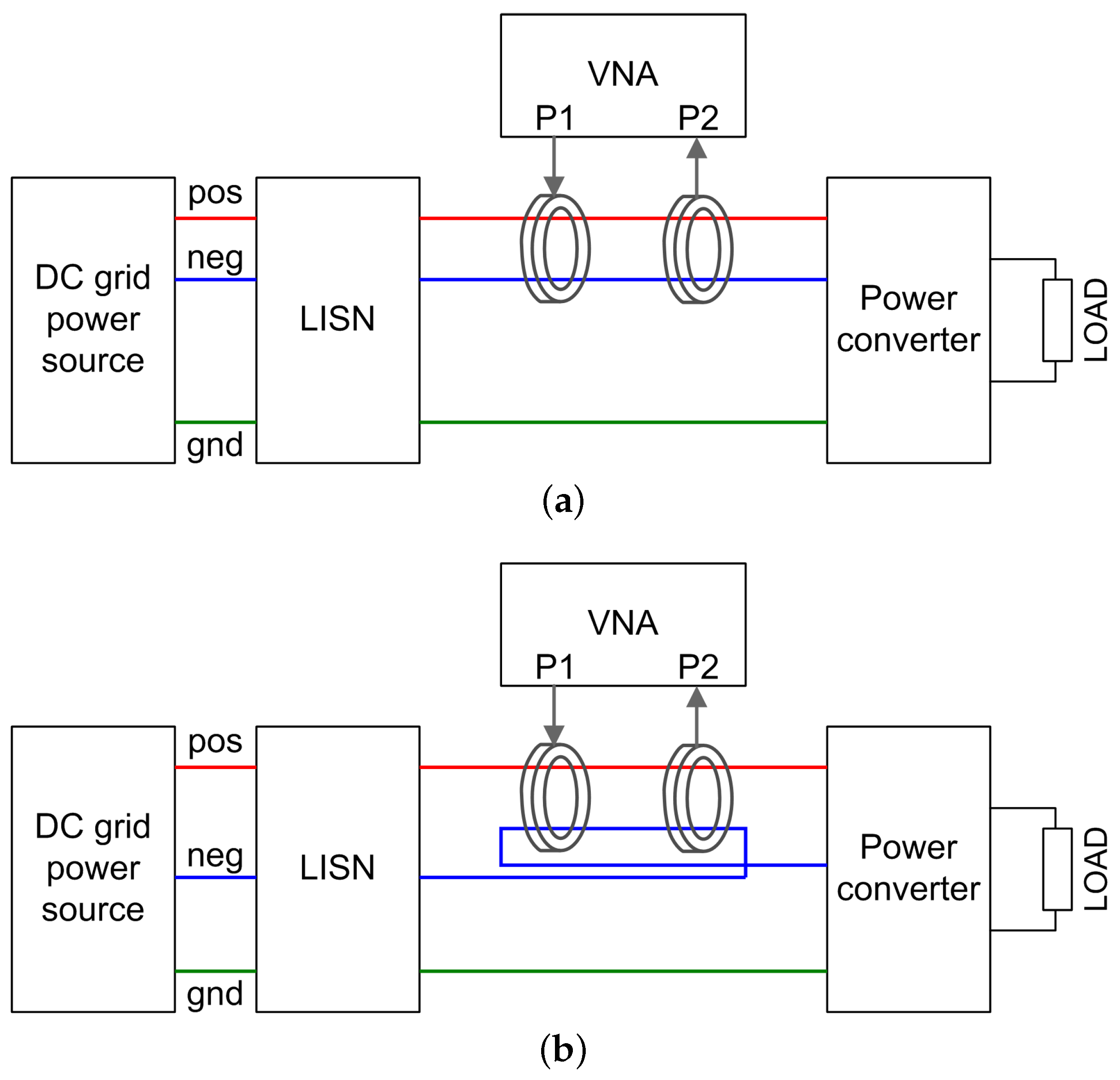
In general, the input impedance of the EUT should be measured in operative conditions (therefore, with the EUT supplied and operating) to get a reliable picture of the real EUT behaviour. This is achieved by applying a test signal and measuring the response at the input port using decoupled channels by means of passive current probes (which are bidirectional and can be used for current injection and current reading) [20,21]. This measurement method is shown in Figure 1, where all relevant elements from an RF point of view are included: the LISN, the connecting wires, and the EUT (power converter), with the two current probes interfaced to the vector network analyzer (VNA).

The advantage of this method is mainly the large signal-to-noise ratio, as the VNA operates in the frequency domain tracking with P2 the swept test signal applied by port P1. Disadvantages consist of the VNA cost, the necessity of having two current probes, and the limitations of the number of points and minimum frequency of some models. For these reasons, a simplified method based on cheaper and commonly available instrumentation is proposed.

2.3. Simplified Method for Impedance and Current Emission Measurement

For the considered supraharmonic frequency range (2 kHz to 150 kHz), the impedance of connecting wires between EUT and LISN may be neglected, especially if they are short. Any other cable connection will be included in the DC grid model discussed below in Section 3. The aim is to replace the active injection of the test signal of the previous method (active impedance measurement) with passive listening of the EUT port. In addition, such a method would provide not only an estimate of the EUT impedance, but also a direct measurement of current emissions; these two pieces of information represent the Norton equivalent circuit that is used then in the DC grid model.

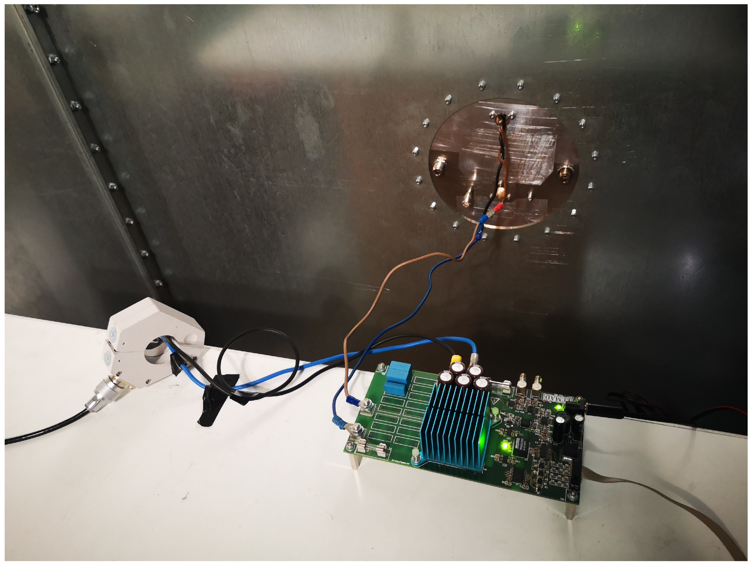
The setup as described in Figure 1b, is limited to the d.m. characterisation; a photo is shown in Figure 2, and the setup elements are described in the caption. In the following, the LISN impedance is indicated by $Z_l$, fed by an ideal voltage source $E_l$ (condition ensured by the use of large-value decoupling capacitors at the LISN input side); the EUT then has an input impedance $Z_e$ with $V_e$, indicating internal distortion voltage associated with distorted current emissions. Measured quantities are the input voltage and current at the EUT port $V_{in}$ and $I_{in}$.

With $V_e$ as the only AC generator in the circuit, the flowing current is determined by the loop impedance:

$$I_{in}=-\frac{V_e}{Z_e+Z_l}=-\frac{V_{in}-Z_e{I}_{in}}{Z_e+Z_l}$$

(1)

Splitting the two halves of the circuit at the left and right of $V_{in}$ and with some manipulation, two, in principle, identical equations are obtained, which, however, differ for unavoidable approximations, noise, and measurement uncertainty, as the two quantities $V_{in}$ and $I_{in}$ are both measured spectra.

$$\begin{array}{cc}\hfill Z_e{I}_{in}+V_e& =-Z_l{I}_{in}\hfill \\ \hfill Z_e{I}_{in}+V_e& =V_{in}\hfill \end{array}$$

(2)

By repeating measurements with different $Z_l$ values, there will be an equal amount of systems of Equation (2) that can be solved by a least square approach.

The proposed Norton equivalent circuit based on the short-circuit current source $I_s$ is preferable to the obvious alternative of the Thévenin equivalent circuit, because a short-circuit condition is more viable in a practical setup, in addition to being available by extrapolation of measurements at moderately low impedance values as in the present case.

With a DC supply, a large capacitor bank between the supply and EUT provides an almost ideal short-circuit path for all relevant AC components in the supraharmonic range and above. The use of large series impedance values (approaching infinite), instead, may compromise the correct operation of the EUT, as it is contrary to good circuit design for switching converters, in addition to being more exposed to the negative effects of parasitic capacitance terms.

3. DC Grid Model

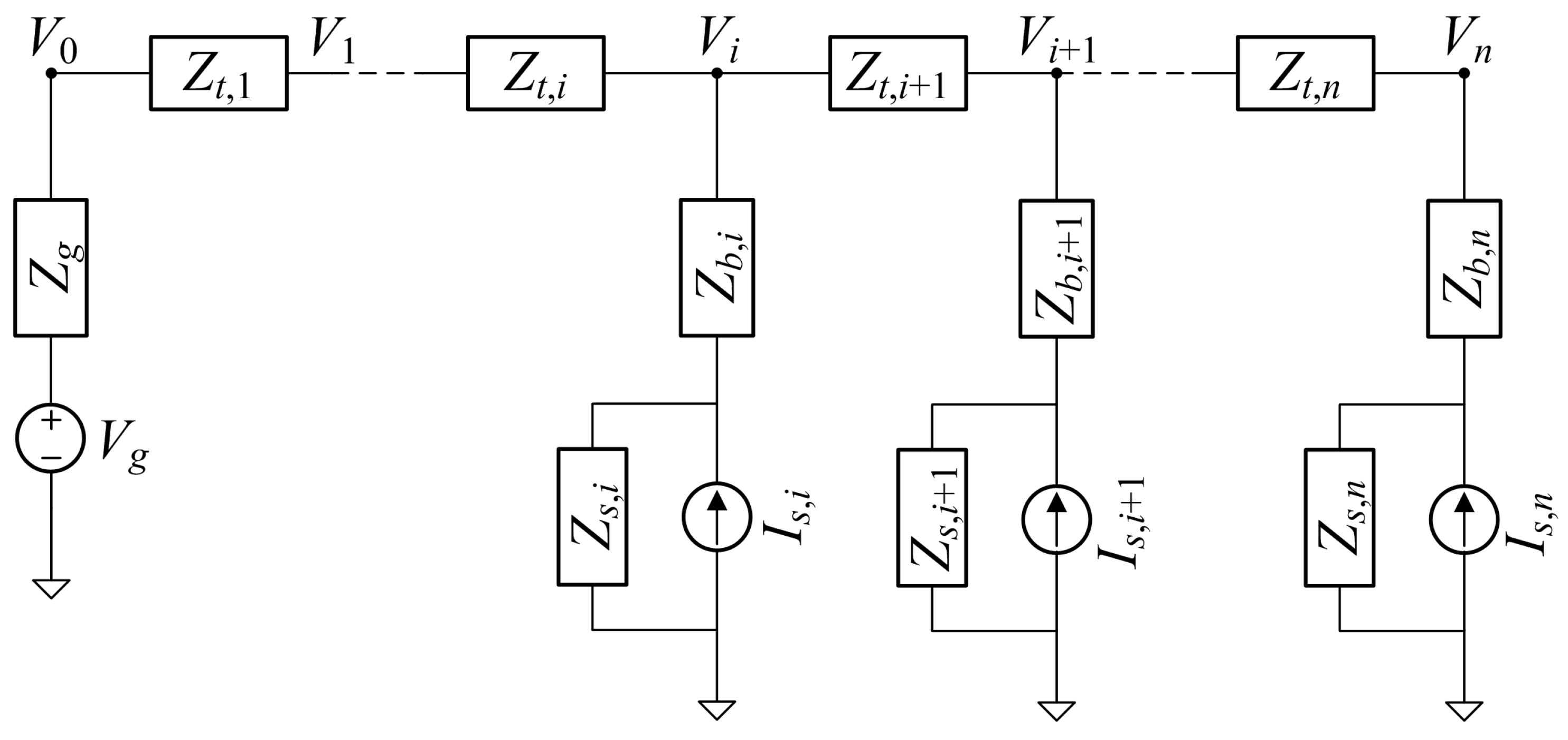
To the aim of combining the disturbance contributions originating from various sources connected at different ports (or tapping points) along the DC grid, the latter may be modelled by means of transmission line branches combined in a ladder network architecture (see Figure 3).

This arrangement is able to model the most common networks used for distribution of power among charging points or WPT coil converters, thus broadly addressing the subject of EV charging: shorting of branch impedance terms $Z_b$ models a straight common-bus distribution, whereas shorting transversal line segments $Z_t$ transforms the ladder into a pure radial network.

Each source is modelled by means of its Norton equivalent circuit, as discussed in Section 2. The noise produced by the network upstream is instead represented by its equivalent Thevenin circuit using the voltage source $V_g$. This is irrelevant, however, to the aim of estimating propagation and superposition of WPT converter disturbance, as long as the feeding network is not characterised by spectrum components at the same frequency.

The DC grid circuit can be solved by symbolic manipulation of expressions and equivalent circuits [22,23] aimed at determining the complete expression of the grid response for the purpose of calculating its frequency response, impulse response. and resonant frequencies (or modes). Alternatively, it may be implemented in a numeric circuit simulator, allowing more flexibility and ease of topological changes by adding/removing elements.

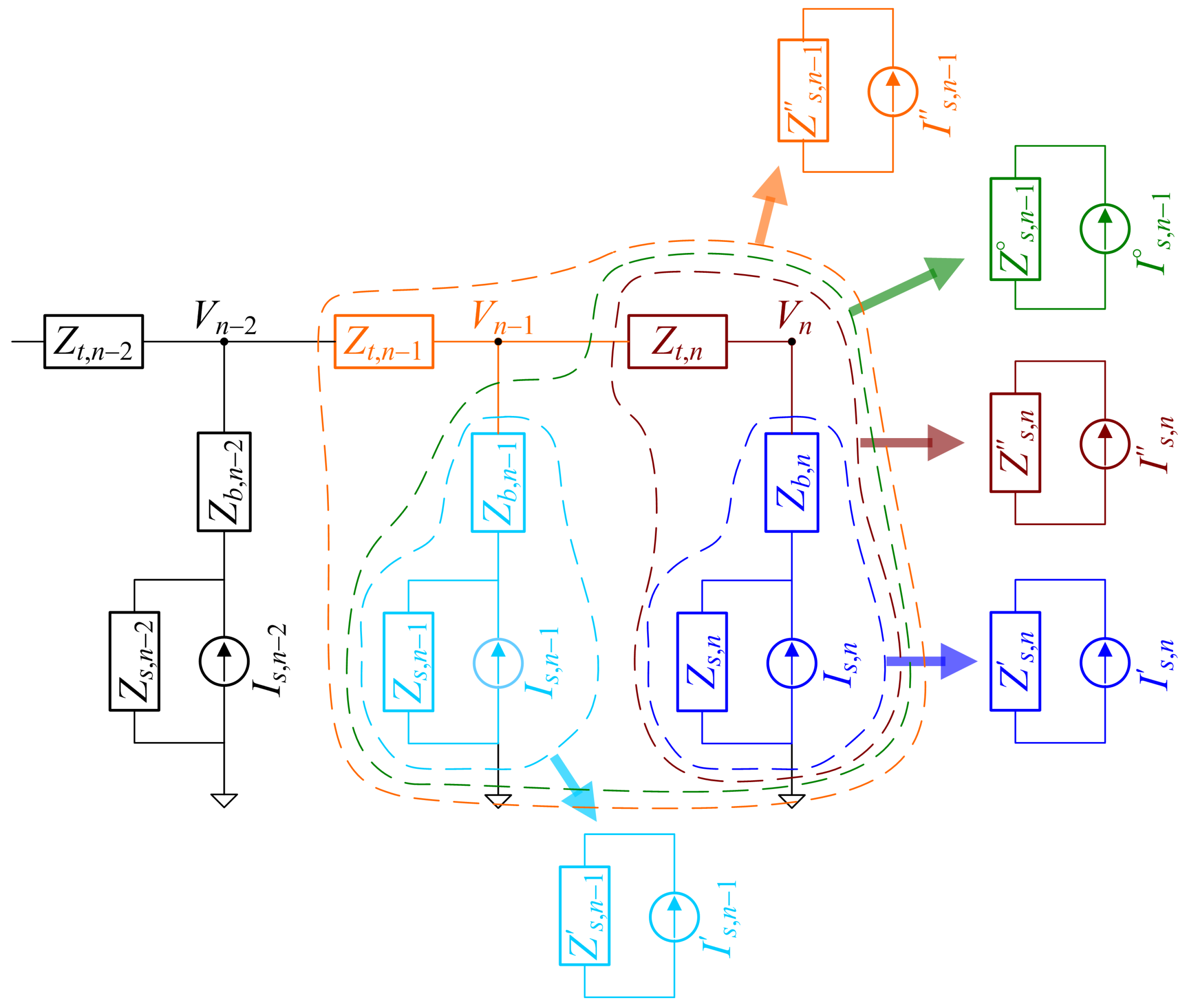
3.1. Iterative Analytical Solution

The network model can be solved iteratively in closed form in two phases:

• Proceeding from the rightmost block of index n back to the feeding point at the left, building at each step a new Norton equivalent model collectively for all blocks downstream of block i;
• The overall Norton equivalent of all combined sources (WPT converters) is realised and connected directly in front of the network equivalent circuit, and the resulting PCC voltage $V_1$ is calculated;
• The second phase then proceeds in the opposite direction, from $V_1$ down to the n block and can then determine the current flowing in each branch (thus in each WPT converter) as resulting from the composition of the internal current $I_i$ and by the application of $V_i$.

The closed-form symbolic solution allows for the calculation of resonant frequencies and the assessment of the statistical distribution of quantities at various points in the network, provided that the probability density functions (pdfs) are known for the current source $I_{s,i}$.

Starting at the nth node and proceeding backwards, there is a first simplification combining the branch impedance $Z_{b,n}$ with the internal source impedance $Z_{s,n}$ (and the same is repeated for any node of index i). In addition, the current flowing along the branch can be calculated, and these quantities are noted with a prime.

$$Z_{s,n}^{\prime }=Z_{b,n}+Z_{s,n}$$

(3)

$$I_{s,n}^{\prime }=I_{s,n}\frac{Y_{b,n}}{Y_{b,n}+Y_{s,n}}$$

(4)

where “Y” is the admittance terms, reciprocal of the respective impedance terms with same notation.

The equivalent branch impedance and current are then combined with the line impedance term $Z_{t,n}$, yielding terms indicated with a double prime.

$$Z_{s,n}^{″}=Z_{t,n}+Z_{s,n}^{\prime }$$

(5)

$$I_{s,n}^{″}=I_{s,n}^{\prime }\frac{Y_{t,n}}{Y_{t,n}+Y_{s,n}^{\prime }}$$

(6)

When combining these terms with those of the previous source block (here with index $n-1$), an additional passage is needed, that of making the parallel between the equivalent downstream with double prime and the new source block under processing; this is indicated with a circle as superscript, not to break the symmetry of prime (source block) and double prime (overall equivalent including line impedance term).

$$Z_{s,n-1}^{\prime }=Z_{b,n-1}+Z_{s,n-1}$$

(7)

$$I_{s,n-1}^{\prime }=I_{s,n-1}\frac{Y_{b,n-1}}{Y_{b,n-1}+Y_{s,n-1}}$$

(8)

$$Z_{s,n-1}^{\circ }=Z_{s,n-1}^{\prime }\Vert Z_{s,n}^{″}$$

(9)

$$I_{s,n-1}^{\circ }=I_{s,n-1}^{\prime }+I_{s,n}^{″}$$

(10)

noting with ‖ the electrical parallel of the two terms.

$$Z_{s,n-1}^{″}=Z_{t,n-1}+Z_{s,n-1}^{\circ }$$

(11)

$$I_{s,n-1}^{″}=I_{s,n-1}^{\circ }\frac{Y_{t,n-1}}{Y_{t,n-1}+Y_{s,n-1}^{\circ }}$$

(12)

It is easy to see that the group of Equations (7)–(12) defines a recursive structure that is applicable anywhere, providing n is replaced by i.

The above simplifications of the network electrical circuit are graphically described in Figure 4.

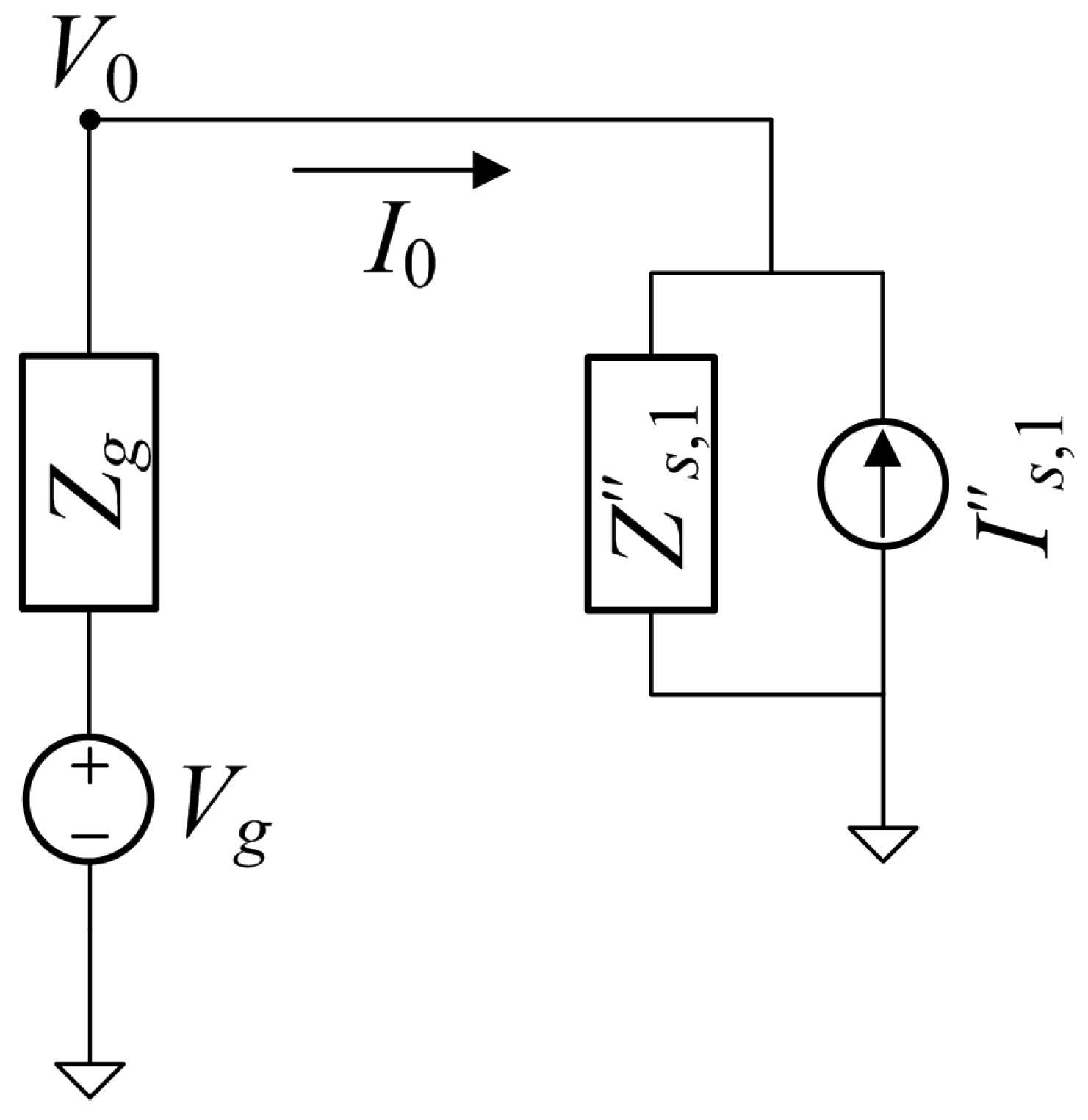
When the subscript $i-1$ reaches 1, the so obtained $Z_{s,i-1}^{″}$ term is presented to the network Thevenin circuit $V_g$ and $Z_g$, together with the equivalent total current $I_{s,i-1}^{″}$, as shown in Figure 5. This allows the calculation of the bus voltage $V_0$ and the total flowing current due to both the network voltage $V_g$ and the source term $I_{s,1}^{″}$.

$$V_0=V_g\frac{Z_{s,1}^{″}}{Z_{s,1}^{″}+Z_g}+I_{s,1}^{″}(Z_{s,1}^{″}\Vert Z_g)$$

(13)

$$I_0=\frac{V_g}{Z_{s,1}^{″}+Z_g}-I_{s,1}^{″}\frac{Z_{s,1}^{″}}{Z_{s,1}^{″}+Z_g}$$

(14)

Proceeding back from the feeding point 0 to the right, the voltage drop along each line segment $Z_{t,i}$ and the current drawn by each equivalent source block $Z_{s,i}^{\circ }$ are calculated recursively, going then into the details of the source blocks of the same indices i and $i+1$.

$$V_1=V_0-Z_{t,1}{I}_0$$

(15)

For the block $Z_{s,1}^{\circ }$, observing that it is the parallel of two blocks, containing $Z_{s,1}^{\prime }$ and $Z_{s,2}^{″}$, we may write:

$$I_{Z_{s,1}^{\prime }}=\frac{V_1}{Z_{s,1}^{\prime }}{I}_{Z_{s,2}^{″}}=\frac{V_1}{Z_{s,2}^{″}}$$

(16)

Putting together the so calculated current provided from the grid $I_{Z_{s,2}^{″}}$ and the one provided locally $I_{s,2}$, it is possible to calculate the new voltage drop along the next line segment:

$$V_2=V_1-Z_{t,2}(I_{Z_{s,2}^{\prime }}-I_{s,2}^{\prime })$$

(17)

This can be put in a generic form for the ith block, to allow for writing the iterated calculation of the current terms, as shown in Equation (16) for the first block.

$$V_i=V_{i-1}-Z_{t,i}(I_{Z_{s,i}^{\prime }}-I_{s,i}^{\prime })$$

(18)

$$I_{Z_{s,i-1}^{\prime }}=\frac{V_{i-1}}{Z_{s,i-1}^{\prime }}{I}_{Z_{s,i}^{″}}=\frac{V_{i-1}}{Z_{s,i}^{″}}$$

(19)

3.2. Numeric Solution with Circuit Simulator

As said, this iterative solution allows the analytical determination of the transfer functions and the assessment of the network response and frequency behaviour, such as the presence of resonances. Otherwise, a more pragmatic approach followed in this work to prepare the results shown in Section 5 is that of implementing the ladder model in a circuit simulator that allows manipulation of probability density functions and carrying out Monte Carlo method (MCM) simulation. The choice fell on Simulink, setting electrical parameters and distributions from the MATLAB environment, so with the possibility of using both ideal and measured data for source current and impedance.

Considering the models discussed in Section 2, results in the following sections are extracted for differential mode, that is, the most relevant by extension of the behaviour of harmonic terms. Common-mode terms in the supraharmonic range and above are getting more and more important [7], and this represents the natural extension of the presented model.

It is noted that the Simulink model runs in the time domain, whereas the expressions above are elaborated in the frequency or Laplace domains. Sources will thus be realised starting from a frequency domain representation as a mix of phasor currents:

$$i_{s,i}=\sum _{k=1}^K{A}_{k,i}sin(2\pi f_{k,i}t+{\beta }_{k,i})$$

(20)

indicating with i the index of the source of emission and with k the index sweeping the set of the K relevant spectral components of amplitude $A_{k,i}$, frequency $f_{k,i}$, and phase ${\beta }_{k,i}$. Although in principle this set may be extended to the entire frequency range when using measured data, it may be limited to the most relevant components.

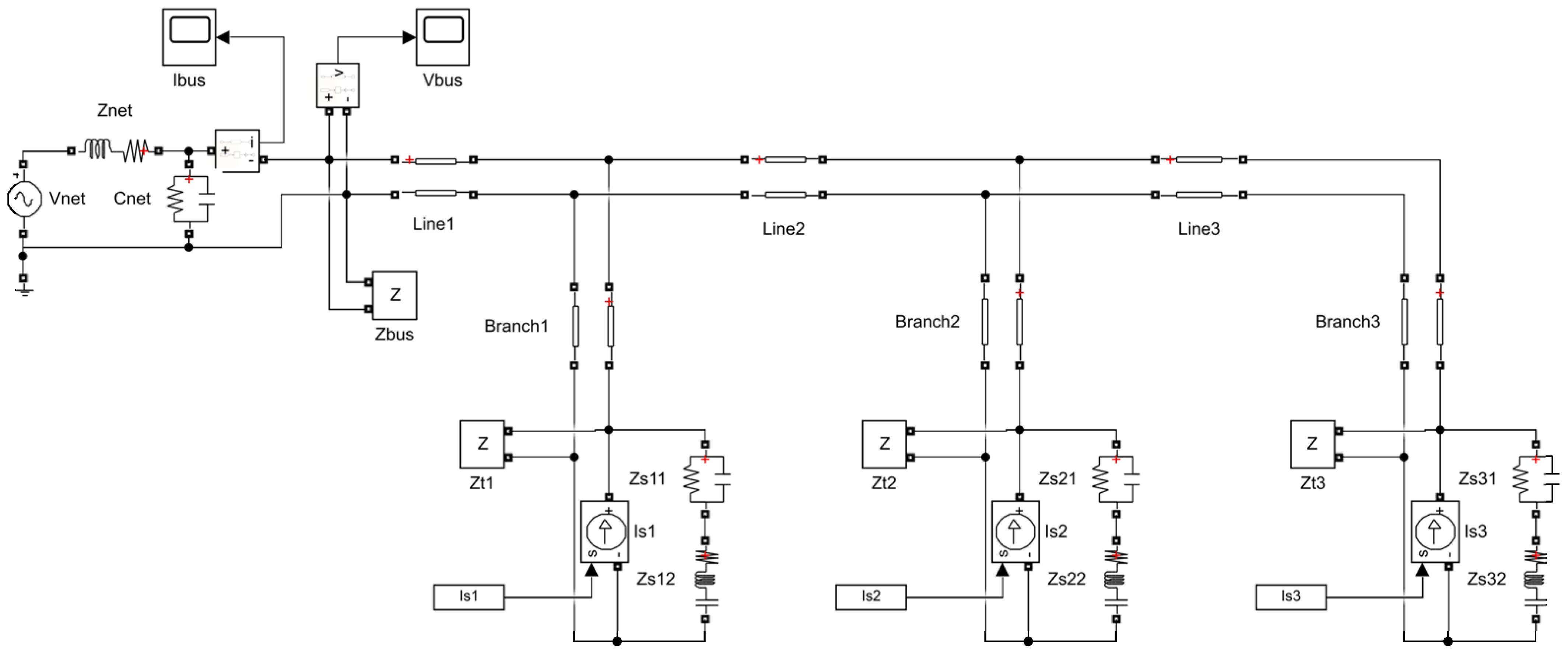
Impedance terms in Simulink using Simscape must be implemented with series and parallel RLC blocks and transmission line blocks for lumped and distributed parameter elements, as shown in Figure 6. Lumped parameter elements are, namely, the input impedance of each source block, i.e., the WPT converter, in addition to the network impedance $Z_g$ at the feeding point. The identification of the measured impedance is thus forced to use a limited number of degrees of freedom, but this is reasonable if considering supraharmonics in differential mode. Distributed parameter elements are exemplified by the connecting cables that can be well modelled with the noted Simscape transmission line blocks.

4. Measured Emissions and Converter Model Identification

The used data acquisition system is a Rohde & Schwarz oscilloscope exploiting three of its four channels to connect two voltage channels and one current channel, the latter exchanged between differential-mode and common-mode current reading due to contingency, as there is only one available current probe. Signals are sampled with a 5 MHz sampling frequency that, keeping a 200 ms time duration for each acquisition, amounts to 1 million samples per channel; that is the limit of the oscilloscope.

Conducted emissions have been measured using the custom LISN prototype implementing different levels of line impedance, at about 0.2 Ω, 0.6 Ω, and 0.6 Ω + 10 μH. The three LISN modes have been verified using an impedance analyser, providing the frequency response in magnitude and phase for each of the two supply lines, positive and negative.

The analysis is focused on differential mode (d.m.) emissions, for which the relevant LISN impedance is the d.m. one. Converter emissions have been measured as (see Figure 2 for a photo of the setup):

• Unsymmetrical voltages, $v_p$ and $v_n$, taken using oscilloscope voltage probes connected between each supply line and ground; such voltage probes are absolutely suitable considering the frequency range of 2 kHz to 150 kHz on which we focus in the present analysis;
• Differential-mode current measured with a Rohde & Schwarz EZ-17 clamp-on current probe; the probe factor is included once the time–domain signals are transformed into frequency domain.

For the creation of the Norton equivalent circuit for the connected converters as sources of emissions, the key elements to address are two:

• Identification of the converter internal impedance as provided by Equation (2);
• Extrapolation to zero-impedance condition that cannot be achieved in normal measurements, as the supply system and connections have their own impedance; this method is preferable to the alternative Thévenein method, as discussed previously in Section 2.

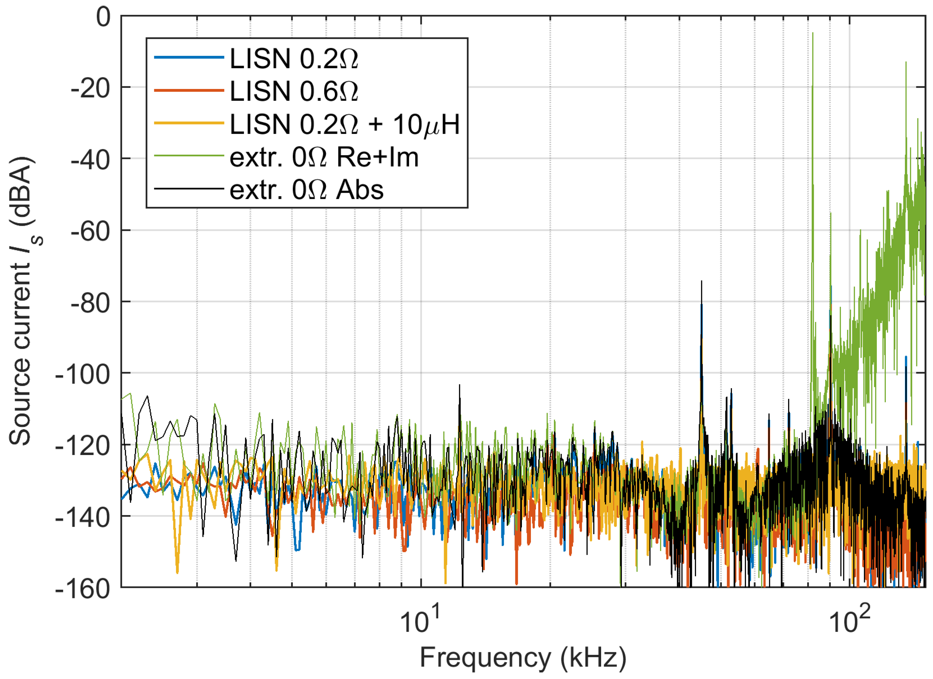
The results of the extrapolation to the 0 Ω condition are shown in Figure 7, where two methods are considered: extrapolation of the absolute value and of the real and imaginary parts, taken separately, indicated by the black and green curves, respectively.

It is observed that the curve obtained by the real + imaginary parts extrapolation is not consistent with the black curve based on amplitude above approximately 90 kHz.

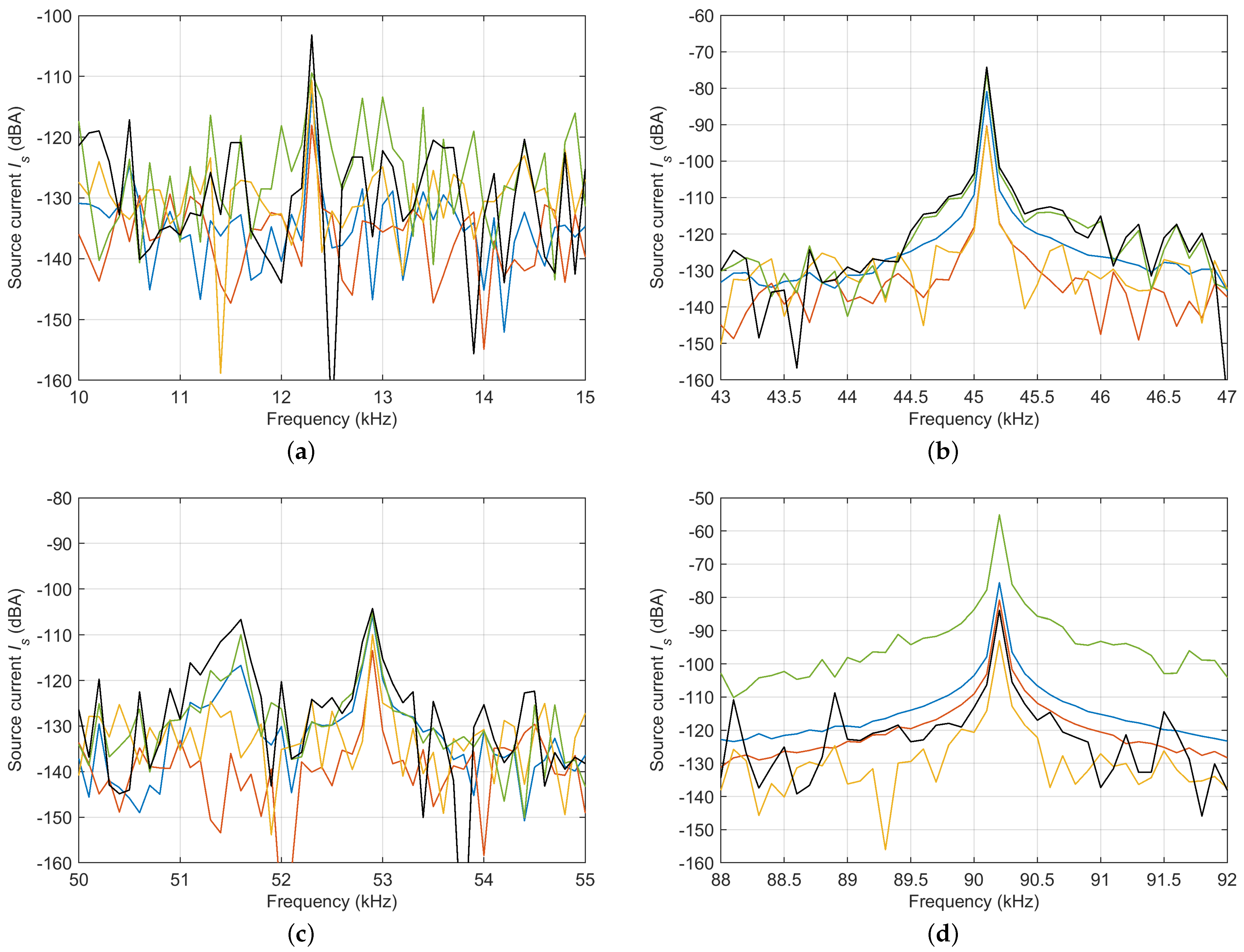
Because the behaviour of extrapolation is not consistent over the entire frequency range, zooms of smaller frequency intervals are reported in Figure 8. It is possible to observe that, at coherent components of emission, the behaviour is as expected, with the extrapolated $I_s$ values larger than the measured ones at the three LISN conditions. Other incoherent components related to noise can instead behave differently (they are visible around the main components in each of the four insets of Figure 8). An exception is observed at 90.2 kHz, where extrapolation carried out considering the absolute value does not provide a maximum value, but an intermediate value between measured components.

The EUT impedance has been determined by solving Equation (2) with a least mean square (LMS) approach, operating a trade-off between a suitable number of independent measurements (observations) and the minimization of effort related to the construction of a different LISN configuration for each of such measurements: the three 0.2 Ω, 0.6 Ω, and 0.6 Ω + 10 μH configurations backed up by two, in principle identical, but dissimilar, $V_{in}$ and $-Z_l{I}_{in}$ measured quantities, has provided a sufficient set of data.

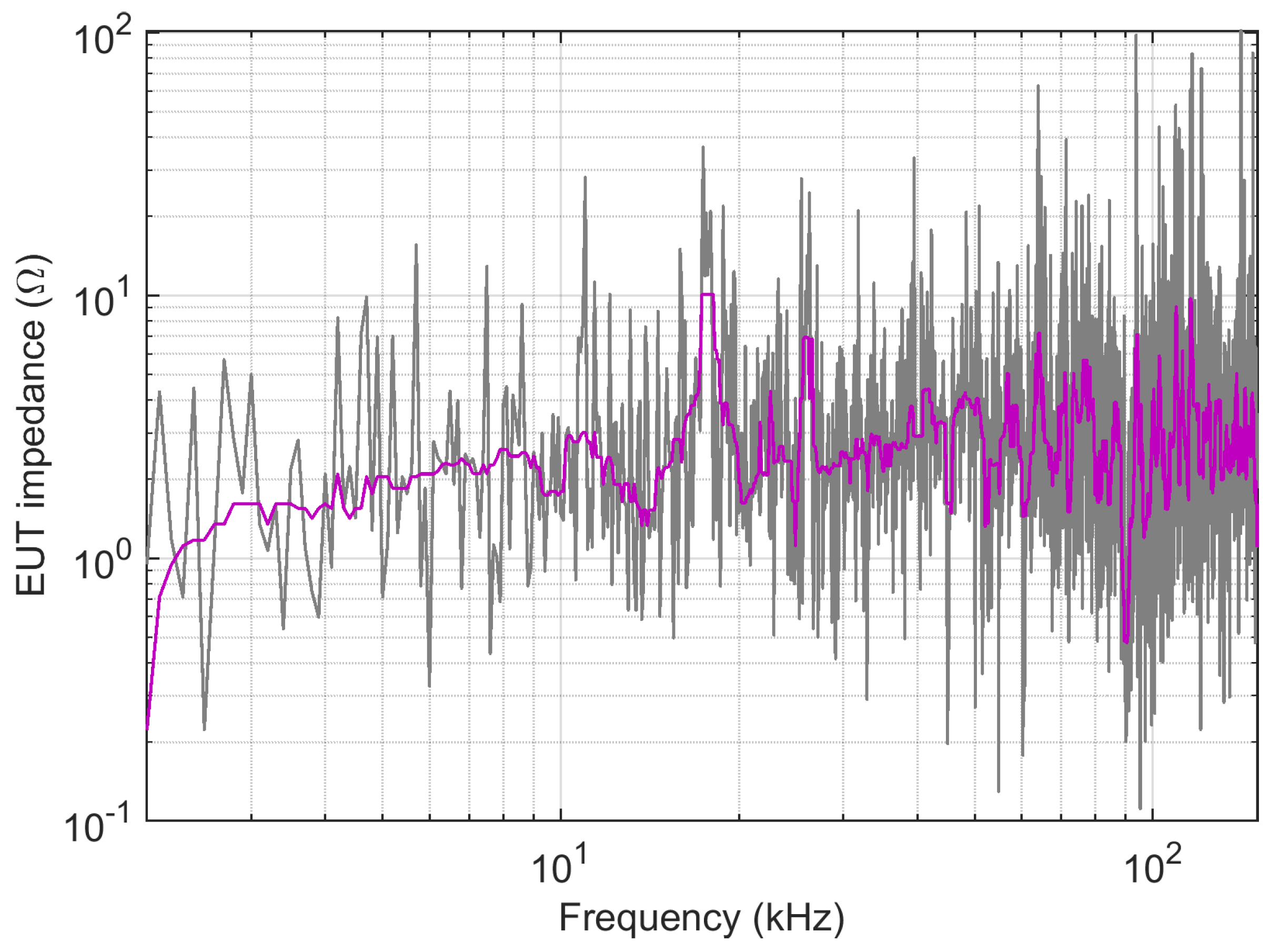
The method should distinguish between coherent and incoherent spectral components, due to emissions and noise, respectively, and use only the former for the estimate of the EUT impedance. With a low signal-to-noise ratio, it is not possible to use the amplitude criterion to separate these two sets of components. Rejection of variability due to the inclusion of incoherent components is then achieved by using a median filter that removes outliers, as shown in Figure 9 using a filter width of 15. The resulting filtered profile has the expected overall profile increasing slightly with frequency with a resonant behaviour due to the input filter at approximately 20 kHz. Parasitic capacitance terms will possibly reduce the input impedance at higher frequency, but they are much more relevant for common-mode impedance.

5. DC Grid Simulation and Combined Disturbance Assessment

Monte Carlo simulations are carried out by a MATLAB script that solves the DC grid electric circuit by using Simulink:

• First, all the parameters of the DC grid components are initialized, such as per-unit-length parameters of cables, current $I_s$, and impedance $Z_e$ of converters, etc.
• The Monte Carlo simulation is then started by generating the first set of $I_s$ waveforms, each built according to Equation (20) with amplitude ($A_1$, $A_2$, and $A_3$) and frequency ($f_1$, $f_2$, and $f_3$) and random phase: three frequency values are considered ($f_1=$ 10 kHz, $f_2=$ 20 kHz, and $f_3=$ 50 kHz) covering well the supraharmonic frequency interval and in particular bracketing a resonance phenomenon occurring in the DC grid; the selected amplitude value is 100 mA for all three components, in line with values commonly measured at the interface of EV chargers [14,17,24].
• The circuit simulation is started from within the script by calling the corresponding .slx Simulink file; when the circuit simulation is completed, the control is returned to the MATLAB script that collects the bus electric quantities.
• Simulations are repeated by looping the generation of $I_s$ signals with random phase, the circuit simulation, and the accumulation of the results.

Another case study is a DC grid featuring ten connected converters, simulated and managed in the same way.

The parameters and quantities are described in

Table 1. Parameters of the Simulink DC grid model and MCM simulations.

Parameter	Value
DC grid intake impedance $Z_{net}$	(1 Ω, 10 μH)‖10 μF
Cable impedance $Z_t$ (1 km)	(0.64 Ω, 0.5 μH, 0.14 μF)
Cable impedance $Z_b$ (1 km)	(0.64 Ω, 0.5 μH, 0.14 μF)
Line segment length	100 m or 5 m
Source current $I_s$ amplitude	100 mA
Source current $I_s$ frequency	$f_1=$ 10 kHz, $f_2=$ 20 kHz, $f_3=$ 50 kHz
Number of connected sources	3 or 10

.

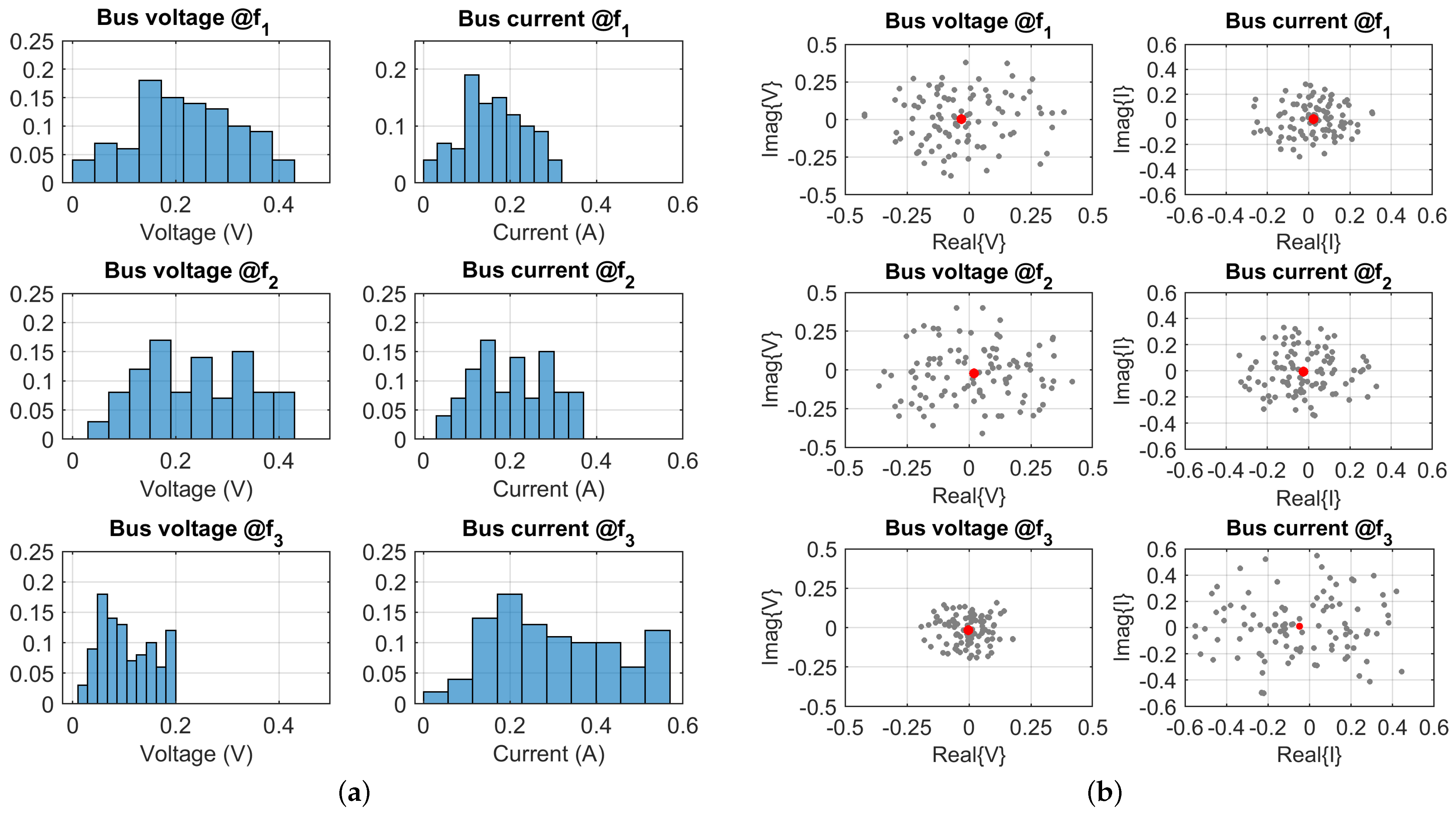
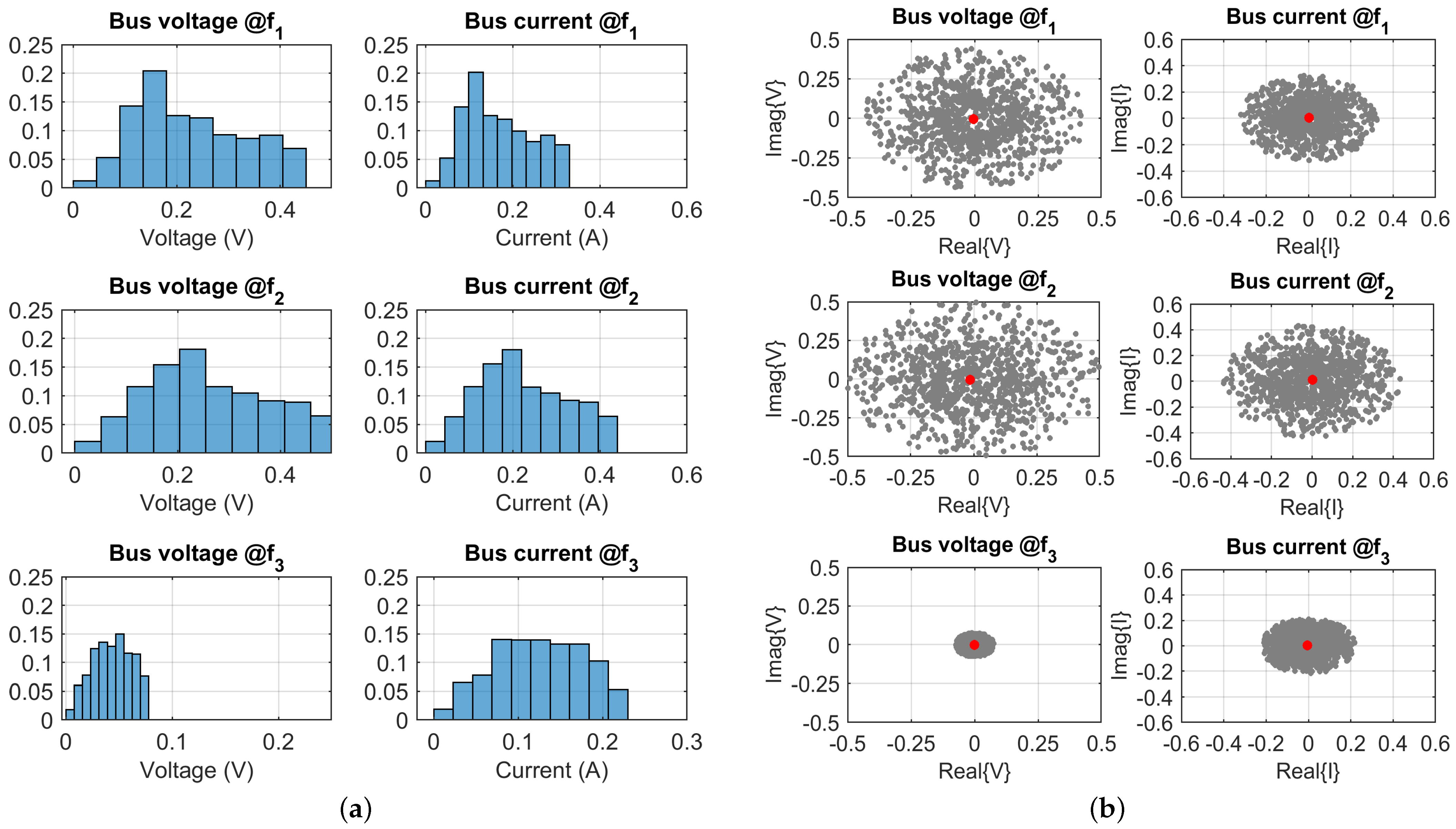
Results are shown in terms of histograms of absolute value and scatter plots of the real and imaginary parts of the bus voltage and current.

By comparing Figure 10a and Figure 11a, it may be concluded that 100 trials with 3 connected WPT converters (i.e., 3 sources of emissions) are not sufficient for an accurate evaluation of distribution of the two bus quantities, voltage $V_0$ and current $I_0$.

This is confirmed by looking at Figure 10b, where the distribution of grey points is somehow uneven, but most of all the red points of the average are slightly offset from the center of the overall cloud of points, that is, the origin. The analysis of the 3-sources configuration is thus carried out using 1000 trials.

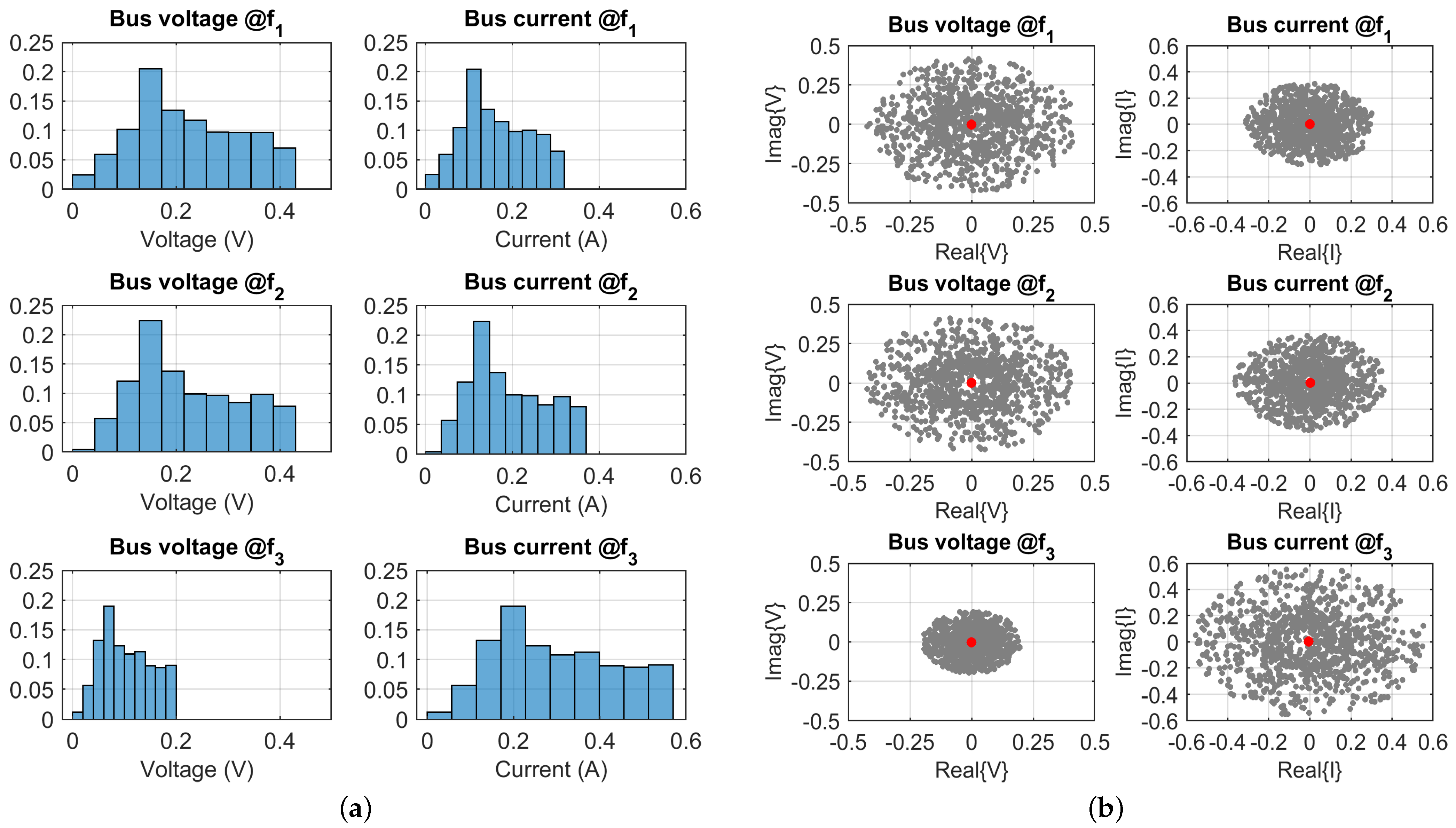
The recently noted almost null overall average does not mean that at each trial the distribution of phases is such to give a balanced distribution leading to a perfect compensation of the emissions from the connected converters, as demonstrated by the distribution of the absolute values. Rather, it is expected that, with an increase in the number of connected converters, the phases of source current will be more evenly distributed and more balanced at each trial. This is discussed later for the case with ten connected converters.

By observing the histogrammed distributions in Figure 11a, it may be immediately noticed that near $f_3$ the grid undergoes an anti-resonance, thus changing the expected inductive increase of impedance with frequency. The bus current consistently features values as large as 400 mA to 500 mA and a lower voltage, approximately half of that observed at the first two frequencies, $f_1$ and $f_2$. The same is evident looking at the scatter plots of Figure 11b, providing a larger cloud of points for $I_0\left(f_3\right)$ (although much denser towards the origin) and a compact smaller cloud of voltage points.

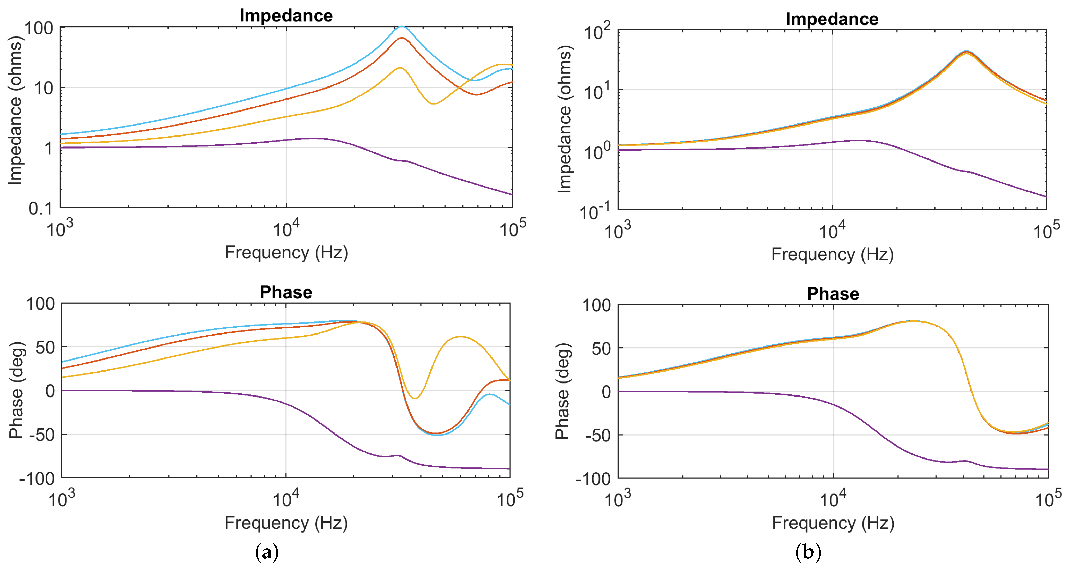
To demonstrate this behaviour, the grid impedance curves have been calculated as seen from the three different converters, as shown in Figure 12: when the grid segments after the first one have negligible length and the converters are connected in proximity, the curves show almost a maximum of the impedance at approximately 50 kHz, whereas when they are distributed evenly with 100 m separation, the impedance curves show progressively an anticipation of the anti-resonance when moving towards the last farthest converter, which sees a minimum of impedance at approximately 45 kHz (yellow curve).

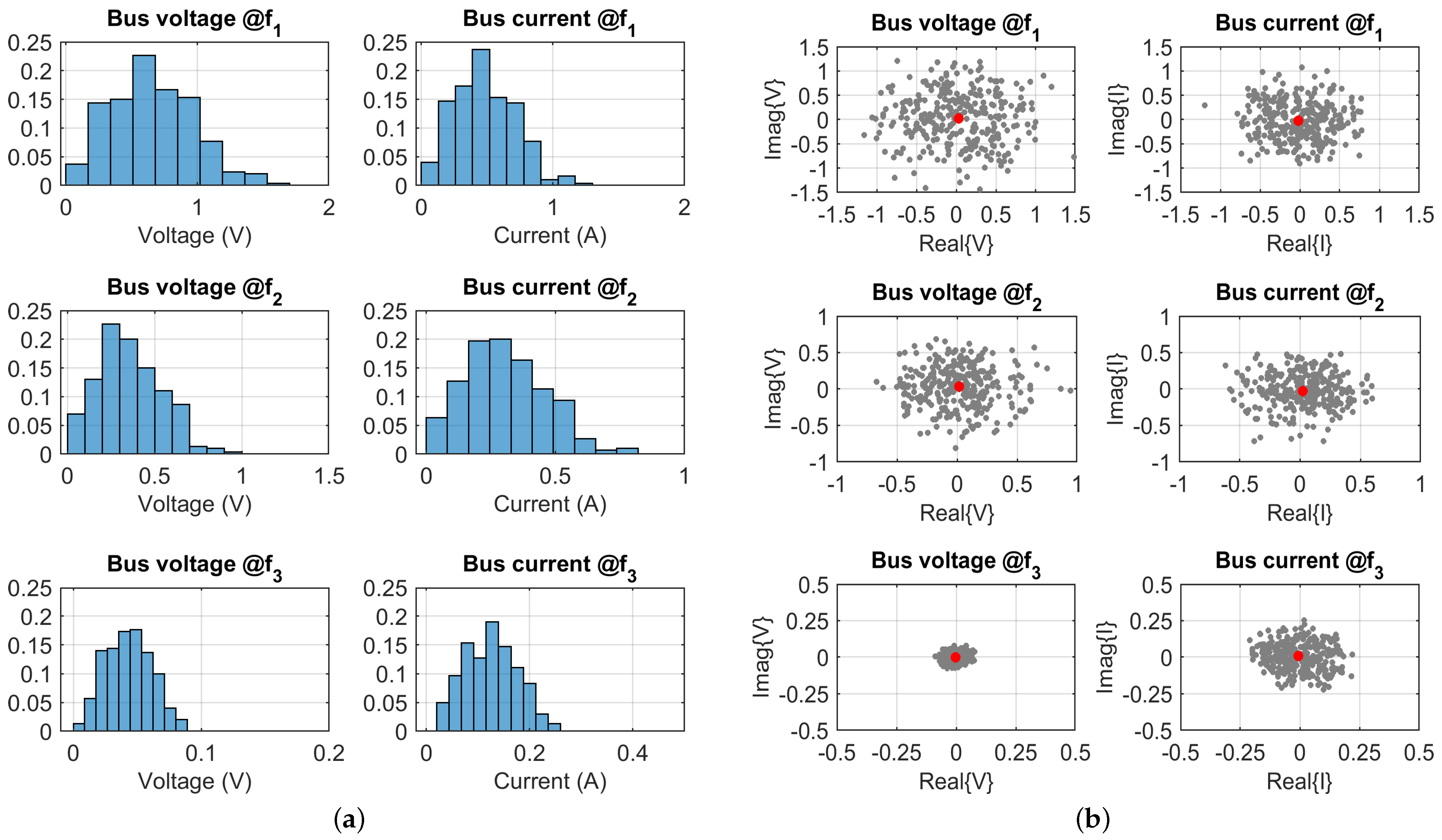
Regarding compensation between sources undergoing a random phase displacement of their emission components, one more degree of freedom is represented by the impedance of the grid segments $Z_{t,i}$ between their connection points, which is a consequence of the relative physical distance (and cable length) between them. This affects not only the impedance response of the grid (as shown in Figure 12), but also the attenuation of each emission component when combined with the others.

Thus, two simulations with the 3-source circuit were carried out, one separating sources with 5 m of cable and another one with 100 m: Figure 11 refers to the 100 m case (separated converters), whereas Figure 13 refers to proximal converters (with 5 m of grid cable between connecting points). In the latter case, there is a greater deal of compensation for the $f_3$ component, which is the one most susceptible to the attenuation caused by cable capacitance: as all $I_s\left(f_3\right)$ components have similar amplitude, they provide better cancellation when the phase displacement allows. At lower frequency, there is no visible change of the compensating behaviour.

Table 2. Measures of dispersion of the MCM simulations for the three-converter network with 100 m of line cable separation between converters.

Quantity	Mean			std
	Real	Imag	abs	Real	Imag	abs
Bus voltage @ $f_1$	−0.0008	−0.0005	0.2214	0.1699	0.1753	0.1028
Bus current @ $f_1$	0.0005	0.0005	0.1635	0.1257	0.1294	0.0760
Bus voltage @ $f_2$	−0.0014	0.0015	0.2218	0.1766	0.1683	0.1013
Bus current @ $f_2$	0.0017	0.0005	0.1911	0.1446	0.1526	0.0873
Bus voltage @ $f_3$	−0.0005	−0.0022	0.1045	0.0804	0.0826	0.0484
Bus current @ $f_3$	−0.0062	0.0017	0.2983	0.2355	0.2296	0.1383

and

Table 3. Measures of dispersion of the MCM simulations for the three-converter network with 5 m of line cable separation between converters.

Quantity	Mean			std
	Real	Imag	abs	Real	Imag	abs
Bus voltage @ $f_1$	−0.0050	−0.0049	0.2282	0.1714	0.1841	0.1057
Bus current @ $f_1$	0.0027	0.0044	0.1686	0.1274	0.1353	0.0781
Bus voltage @ $f_2$	−0.0145	−0.0055	0.2614	0.2073	0.1991	0.1203
Bus current @ $f_2$	0.0014	0.0133	0.2252	0.1736	0.1766	0.1037
Bus voltage @ $f_3$	−0.0014	−0.0015	0.0436	0.0334	0.0335	0.0184
Bus current @ $f_3$	−0.0041	0.0040	0.1244	0.0958	0.0951	0.0525

report the numeric values.

Simulations carried out for the ten-source scenario allow for drawing the following conclusions. Because the emissions of ten sources are collected at the DC grid intake, the reference current is ten times that of a single source, so 3.33 times larger than that for the three-source case. The amplitude histograms are more compact if comparing the position of the peak (the bin with maximum probability) with the spread of values: we pass from slightly less than 50% for three sources to about 30% for the ten sources, roughly proportional to the expected square root of the ratio of the number of sources, i.e., 1.8. The histograms of Figure 14 exhibit also a more pronounced tail, showing a significant reduction following the noted peak of the distribution.

This method of analysis has proven to provide relevant results for the composition of the emission spectra with the following points:

• The frequency response of the grid can influence the behaviour of the various contributions at the point of common coupling (the DC grid intake), as they may be attenuated or amplified depending on the behaviour of the impedance curve (between the extremes of a resonant and anti-resonant behaviour, as demonstrated for the $f_3=$ 50 kHz component);
• The random phase distribution allows for compensation between sources of emissions, provided that their number is sufficient to derive solid statistical compensation;
• Additional degrees of freedom may be provided if also amplitude and frequency can undergo a random behaviour, for which an estimate of their probability distribution function can be assigned and implemented in a MCM simulation.

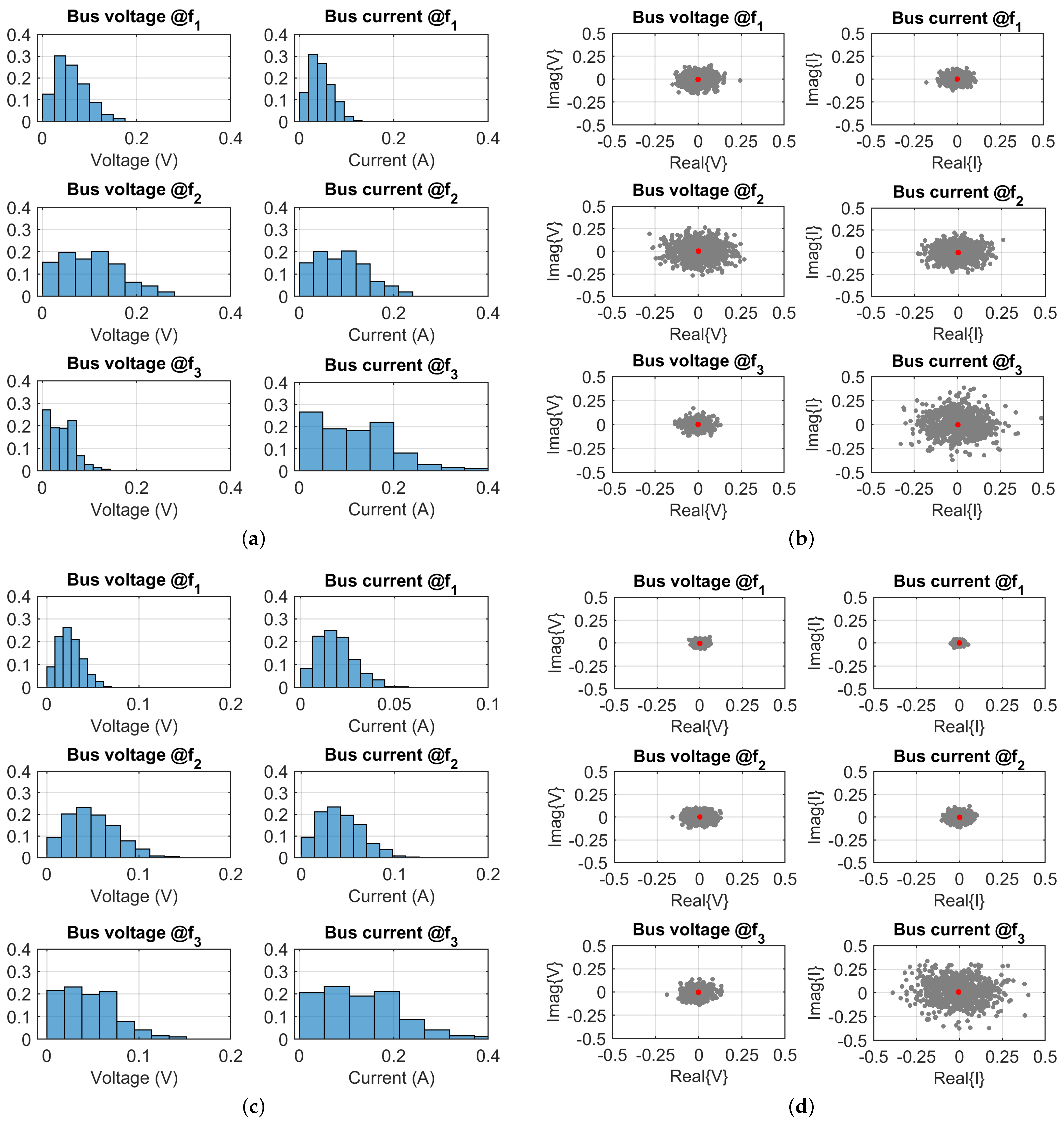
Whereas amplitude changes are natural for a scenario with variable operating conditions (namely absorbed power, temperature of the specific converter, etc.), the random shift of the frequency of the spectral components must be weighted by the adopted resolution used for the Fourier analysis of the signals. Two components that can be resolved at a finer frequency resolution are counted as one when the width of the frequency bin increases, although they get composed within it with a slightly different relative weight. This is demonstrated in Figure 15.

The applied random $\pm 1\%$ change to the components frequency translates into a frequency shift that is proportional to their frequency value, namely $\pm 100$ Hz, $\pm 200$ Hz, and $\pm 500$ Hz for $f_1$, $f_2$, and $f_3$, respectively. The two frequency resolution values used for the Fourier analysis of simulated signals are 200 Hz (results reported in Figure 15a,b) and 500 Hz (results reported in Figure 15c,d). The beneficial effect of the larger frequency resolution consists of a better achievement of compensation between sources because of the higher probability that frequency shifts farther away fall inside the same frequency bin and are de facto summed algebraically together, rather than occurring in adjacent bins. Because the possible victims of such emissions are not narrowband systems, it is natural to expect that large frequency resolution values are more suitable to assess the overall interference.

6. Conclusions

The work has considered the problem of characterizing the behaviour of WPT power converters with the objective of determining an equivalent circuit for conducted emissions, suitable for later use in circuit simulation. The purpose of the circuit simulation of an entire DC grid feeding a significant number of such converters is the verification of aggregation and the extent of mutual compensation between the different sources of conducted emissions.

Converters are not synchronized to a main grid frequency for two reasons: the grid is operated at DC and, in any case, there is no reason to synchronize high-frequency conversion components located at tens or hundreds of kHz even with an AC grid. This supports the assumption of random phase distribution of such components, as was analysed in this work.

The proposed equivalent circuit representation is that of a Norton equivalent, using extrapolation of measured current to the 0 Ω condition. The identification of the equivalent converter impedance is carried out by least mean square identification. Results are satisfactory, with a great deal of work to reject the effect of incoherent spectral components caused by measurement noise. The proposed methods are extrapolation of absolute value of measured current components and of the real and imaginary parts separately, showing some sensitivity to incoherent spectrum components, which remains the main challenge. Using the absolute value gave the best performance. An alternative active method, already proposed in the literature [20,21], is that of using a sweeping test signal, provided by a second current probe used as an injecting point: in this case, the measurement should use a frequency domain instrument (such as vector network analyzer) to exploit the so provided larger signal-to-noise ratio. This technique has much better performance in terms of accuracy and insensitivity to disturbance. However, the advantage of the proposed method is that it is passive and uses less expensive instrumentation, already used to carry out the emissions measurements.

The composition and partial compensation of emissions have been demonstrated with Monte Carlo method simulations of selected network configurations, showing the effect of the distribution cables and network resonances, while providing the statistical distribution of resulting grid quantities, namely, the voltage and current phasors at the DC grid intake. The analysis has focused on the behaviour of the injected spectral components, located at three conveniently spread frequencies, namely 10 kHz, 20 kHz, and 50 kHz. The results show that the 50 kHz is close to a network resonance that takes place for a moderate, but not negligible, length of connecting cables, for a total span on the order of 300 m. Wider grid extensions will, of course, lower resonance frequencies more deeply into the first portion of the frequency interval, where emissions are expected to be stronger. As the method is equally applicable to DC and AC grids and also for static EV charging applications, extensions in the kilometer range cannot be excluded, making the interaction with grid resonance more complex; in this case, the proposed analysis is strongly recommended. The obtained results demonstrate the extent of compensation between converters in a realistic scenario, where connecting cables and physical separation have been considered, as opposed to [19], where converters are all concentrated at one point. Past contributions discussed some experimental results [17,24] but never proposed an integrated approach that includes variable converter emissions and network configurations and the statistics of their conducted emissions.

In line with this last consideration, future developments of converter characterization integrated with grid modeling for combined aggregation and statistical analysis are: the extension to AC grid cases, the inclusion of more variability depending on converter operating conditions, and the validation with real scenarios (where extensive measurements of network quantities are a necessity, including long observation times to derive meaningful statistics to compare with the outcome of MCM simulation results).