Machine Learning in Operating of Low Voltage Future Grid

Abstract

The article is a continuation of the authors’ ongoing research related to power flow and voltage control in LV grids. It outlines how the Distribution System Operator (DSO) can use Machine Learning (ML) technology in a future grid. Based on supervised learning, a Selectively Coherent Model of Converter System Control for an LV grid (SCM_CSC) is proposed. This represents a fresh, new approach to combining off and on-line computing for DSOs, in line with the decarbonisation process. The main kernel of the model is a neural network developed from the initial prediction results generated by regression analysis. For selected PV system operation scenarios, the LV grid of the future dynamically controls the power flow using AC/DC converter circuits for Battery Energy Storage Systems (BESS). The objective function is to maintain the required voltage conditions for high PV generation in an LV grid line area and to minimise power flows to the MV grid. Based on the training and validation data prepared for artificial neural networks (ANN), a Mean Absolute Percentage Error (MAPE) of 0.15% BESS and 0.51–0.55% BESS 1 and BESS 2 were achieved, which represents a prediction error level of 170–300 VA in the specification of the BESS power control. The results are presented for the dynamic control of BESS 1 and BESS 2 using an ANN output and closed-loop PID control including a 2nd order filter. The research work represents a further step in the digital transformation of the energy sector.

1. Introduction

An increasing number of authors have published studies which suggest that there are beneficial applications for AC/DC converter systems connected to low voltage grids [1,2,3,4,5,6,7,8,9,10,11,12]. Power flow in an LV grid is controlled to suit the bidirectional nature of their operation. It should be noted that every LV grid is different, due to the number of consumers, its physical parameters, or the number of prosumers. However, a number of patterns are present that have a significant impact on the operation of LV grids, i.e., PV generation power factor (p.f.) and grid capacity [13,14,15,16,17,18,19,20,21].

Poland supports the European decarbonisation process. It currently faces the challenge of reconciling the growth of distributed power generation and its local consumption for sustainable development in the energy system. The use of AC/DC converter circuits in LV grids alone is insufficient for DSOs to achieve the objectives of grid control. The dynamics of the changes in LV grids, due to the load profile and the movement of the sun during the day, require active control of converter P and Q [22,23,24,25,26]. Grid support follow-up systems become insufficient, as they are an improvement to the power/voltage grid parameters at one selected connection point of the AC/DC system [27,28,29,30]. These types of systems work very well in closed microgrid-class systems. An LV grid requires a coherent perspective, with consideration of all its nodal points, especially those at the ends of the lines.

It should be stressed that the transformation of the energy sector will force a paradigm shift in the operation of LV grids. This concerns the operating boundary conditions for PV generation in particular. The objective function for DSOs will be to maximise local generation from the PV in favour of taking this power from the TSO nodes, the opposite of what current practice dictates [31,32,33]. This is due to the volatile prices of fuel, coal and gas, or the availability of hydrogen for central power and energy generation units in the electrical power system [34,35,36,37,38,39,40]. The costs of fuels, the switching of industries to electrical power and its flow from HV to LV will become increasingly expensive. DSOs will be forced to optimally and selectively manage power and energy at the generating sites.

A review of the literature on the subject suggests that there is currently no description of dynamic control for AC/DC converters in LV grids by application of simultaneous decentralised microcontrollers. As an alternative, the literature only indicates the use of BESS by the prosumer and the possibility of cooperation for the LV grid [41,42,43,44,45,46,47,48,49,50].

1.1. Research Gap

• Dynamic management of power flows in the LV grid, with high levels of distributed power generation in prosumer installations. Most papers list the static or emergency operating states due to the objective function;
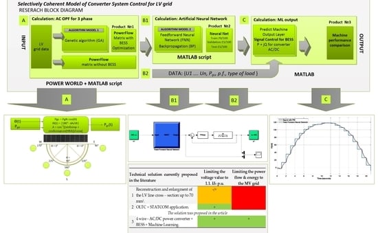
• Application of ANN machine learning models in LV grids for control of AC/DC power converter systems—the research hypothesis presented in this paper;
• Development of new processes for the management of DSO assets in Poland in connection with the increasing digital transformation. New models of operation for actuation and control devices under the operator’s supervision;
• Building an architecture for the logical aggregation of metering data from LV grids, e.g., Advance Metering Infrastructure class meters in offline and online modes.

1.2. Motivation

The motivation for the research was to discover the architecture for the AC/DC converter control and through which algorithms the DSO can achieve the intended objective, being dynamic control of power flows in the LV grid. This means achieving not only a limitation of the increase in voltage ratings at the PV connection points, but also the limitation of the power flows to the MV grid. The proposal was to use regression methods and neural networks (ANN) to predict the P + Q values of a converter system operated to improve the voltage performance of the LV grid.

1.3. Research Procedures

The object of analyses and research work was an actual LV grid (see description in Section 2.1). Power flow analyses were performed in terms of the changes in p.f. $\langle 0.95-1\rangle$, PV power $\left(0-8\right.〉$ kW and load scenarios (see

Table 1. Times of voltage condition overruns of the test object on 22 June.

Scenario	Real Time	Pgc	Type of Load	Power Factor
1	0:50	7.8–8 kW	SF—weekend	1
2	3:10	5.9–8 kW	SF—weekend	0.95
3	3:20	5.7–8 kW	R—week	1
4	4:40	4.3–8 KW	R—week	0.95

). The observations of voltage conditions were the datasets used for machine learning (see

Table 2. Characteristics of the training and test data.

Training Data	Testing Data
Pgc, p.f.: 2d (two-dimensional) Load: 4d (four-dimensional) BESS Predictors: 26d (twenty-six-dimensional) BESS 1 Predictors: 13d (thirteen-dimensional) BESS 2 Predictors: 10d (ten-dimensional)	Pgc, p.f.: 2d (two-dimensional) Load: 4d (four-dimensional) BESS Predictors: 26d (twenty-six-dimensional) BESS 2 Predictors: 10d (ten-dimensional)
Output: 1	Output: Prediction
Scenario: 12	Scenario: 4
Low Voltage grid operation type: BESS and BESS1/2	Low Voltage grid operation type: BESS and BESS1/2

). The training, validation and test data X → ℝ had a single PowerWord data source; however, they were not common sets as they were independent. MATLAB was used as the modelling environment for ANN machines and SIMULINK for the signal control dynamics.

2. Materials and Methods

2.1. Original Infrastructure—Research Environment

In practice, there were two models for DSO management for the on/off actuators or technical parameter control (see Figure 1). The first mode was “A”, or centralised control. The master computing unit performed the parameterisation calculations for a defined condition and objective function. This required building an advanced computing unit, but the calculation results were close to the real ones. In this case, it was voltage optimization of the nN grid nodes for the values of P and Q [51,52,53,54,55,56,57] of the given converter in time window t. The second model, “B”, was decentralised control, which dispersed the decision-making locally in the place where control was required directly. The local unit, a microcontroller, controlled the operation of the converter system in a simplified way, as it was unable to run advanced calculations by itself, as in the case of model A. It was possible to combine the two models as one hybrid. This enabled use of the best features of models A and B. The fixed parameters of the LV grid and its development will eventually be allocated centrally in a dedicated domain environment, while the optimal output set responses for the converter control function will be made local.

With these operational activities and assumed logic of operation, a change was required in the processes relevant to the management of the DSO assets in the LV and MV grids [58,59,60,61]. The LV grid mapped in GIS class systems had to have functionalities which enabled analysis of the power flows with distributed power generation. The purpose of the new functionalities was to collect training data for the building of machines learning local control as a function of the adopted objective. The hybrid operation system for the two possible locations of BESS in the LV grid is shown in Figure 2.

The LV grid model was adopted from the authors’ publication [62], which involved a grid studied for power flows using the PowerWorld environment (the test object). The power generation capacity for a system of PV modules installed by the prosumers changed dynamically with the movement of the sun on a given day of the year. During this work, it was assumed that the day would be 22 June for the geographical location of the LV grid specified below: Latitude: 52.10.04, Longitude: 22.16.17 UTC + 1. A mathematical model of the transition from the PV physical quantities (P_gN) to the actual value P_gc(t) is shown in Figure 3.

Where:

• P_gN—Nominal PV power value per prosumer [kW];
• P_gc—PV generation current capacity [kVA];
• θ—Angular distance between the azimuth and the PV installation;
• A—Azimuth.

PV systems in Poland have typically been installed facing south, allowing the maximum generation capacity to be achieved with θ = 90°. The solar motion (see Figure 3) made the operation of the test object dynamic, due to the change in P_gc(t). As the power flow changed, consequently, the voltage conditions of the test object increased. The determinants for the overrun of temporal voltage conditions, U_n < 1.1 p.u., for the connection points were: P_gc, load and power factor (see Table 1). The data were obtained with the assumption of zero cloud cover and full operational performance for all PVs within the test object. The calculation error compared to the actual data for the tested day could be affected by the ambient temperature, reducing the nominal capacity of the PV panels.

The time-stamped measurement data from the test object had to be transmitted to the BESS controller from the overvoltage overruns according to a 10-min average (see EN-50549-1). This means that a communication line had to be set up with AC/DC PV converter systems for RMS U_n measurement towards the BESS controller. To develop the boundary conditions, the authors assumed 10-min measurement sequences of the test object for time window t of the BESS control (see Table 1).

A review of the scientific literature suggested that On-Load Tap Changer (OLTC) operation had a direct effect on the variation in the RMS voltage value of an LV grid that was highly penetrated by PVs [63,64,65,66,67]. To confirm this, simulations were carried out on the test object. For this purpose, the feasibility of OLTC control was applied with TAP = 2.5% in the ΔU p.u. change from the voltage rating, resulting from the transformer ratio (MV/LV transformer primary voltage rating). The change in voltage ratio was simulated in the PowerWord environment at the TAP:2 upward (5% U_n) and TAP:3 upward (7.5% U_n) positions. Two main scenarios were adopted for the analysis of power flow in the test object: SF and R (see Table 1). The power generation capacity P_gc was 8, 9 and 10 kW per consumer. Figure 4, Figure 5, Figure 6 and Figure 7 show the RMS p.u. voltage waveforms independently for the two branches (Feeder 1: 13 connection points, Feeder 2: 10 connection points).

Analysis of Figure 4: Note the evident improvement in U_n values with TAP-3, even with considerable values of P_gc = 10 kW.

Analysis of Figure 5: Note that for Feeder 1, TAP-3 reduced the overrun of 1.1 U_n to 9 kW. For Feeder 2, there was a reduction at P_gc = 8 kW.

Analysis of Figure 6: Note the evident improvement in U_n values with TAP-3, even with considerable values of P_gc.

Analysis of Figure 7: Note that for Feeder 1, TAP-3 improved U_n only at 8 kW and 9 kW per connection point. For Feeder 2, only TAP-3 provided an improvement, yet only up to a power of P_gc = 8 kW.

2.2. Research Methodology

The Selectively Coherent Model of Converter System Control for LV grid–SCM_CSC, shown in Figure 8, was proposed for the construction of a logic topology for a microcontroller to implement dynamic control of the power flow in an LV grid using an AC/DC power converter system(s) [62]. The model consisted of three instances of operation, presented in three sequential blocks.

The first two instances of the SCM_CSC model had to be made offline and were used to prepare the target control for the third instance. The final instance ran online through a GPU microcontroller-type actuator [88,89,90,91]. The SCM_CSC model was based on Machine Learning (ML) technology by collecting predictors according to a predefined classification and the expected response for the control system.

SCM_CSC Block A—this required offline preparation of two categories of measurement data from the grid system (training data and testing data). The training data were a matrix which represented the prediction data (predictors) with the optimal P + Q selection for the BESS in the hybrid operation system (see Figure 2a,b). The matrix was built based on pre-developed scenarios of the test object operation considering p.f. $\langle 0.95-1\rangle$, apparent power S for PV $\left(0-8\right.〉$ kVA, increment 0.25 kW and the load characteristics on the prosumer side (load–SF/R) [62].

The preparation of the training data for the tests included the selection of the data characteristics and their regularities between each other. Principal Component Analysis (PCA) was used for this purpose [92,93,94,95,96]. The extract of the analysis gave the identified clusters of converging characteristics and their common hierarchical relationship to the BESS, p.f. P_gc.

The analysis showed an existing data linkage between each other, as the future predictors (see Figure 9 and Figure 10). The control variables for the data model (p.f. and P_gc) interacted differently through the hierarchy with the different nodes in the feeders. Furthermore, future prediction would have to learn these relationships in order to recognise them correctly. The datasets presented were systems of non-linear functions. Due to the number of input parameters (16–26) of the predictors, a mathematical description in the form of a polynomial up to the 26th order would be difficult. The ability to control a system through equations of state with this number of variables would be infeasible. To assess the quality of prediction by the future machines and their application, Figure 11 and Figure 12 show the training data distribution separately for BESS and BESS 2. The granularity of the data collected for training had a direct impact on the quality of the control as well as on the distribution of the AC OPF results.

The empty spaces between the data in Figure 11 and Figure 12 would hinder correct machine predictions. Despite the limitations, continuity and predictive validity could be demonstrated. The reason for this work was that the application of machine learning to LV grid data (Table 2) would enable dynamic control of BESS.

3. Results

For analytical purposes, regression-based mathematical models (mdl) were used to verify and compare the validity of machine learning. Measures for the learning quality of a machine were MAPE and MSE [97,98,99,100,101]:

$$\mathrm{MAPE}={\displaystyle \sum }_{t=1}^N\left|\frac{TRAINING DAT{A}_t-Predicte{d}_t}{TRAINING DAT{A}_t}\right|\times \frac{100}{N},$$

(1)

$$\mathrm{MSE}=\frac{1}{N}{\displaystyle \sum }_{t=1}^N\left|{\left(TRAINING DAT{A}_t-Predicte{d}_t\right)}^2\right|,$$

(2)

3.1. Regression Models—Data Training

Three groups of regression-based machines were built for the development of the SCM_CSC product 2. This was because three independent microcontrollers were used, working for the two potential operation systems of the LV grid. One microcontroller was used for BESS at an MV/LV substation and two independent microcontrollers for BESS 1 and BESS 2.

3.1.1. First LV Grid Operation System with BESS

The objective for mdl was to predict the P + Q values for control under BESS in order maintain the voltage condition value. See

Table 3. Computational results for mdl in the operation system of the test object with a single BESS.

Regression Model	MAPE [%]
Gaussian Processes Model—Kernel	0.22392
Stepwise AIC	6.6313
Stepwise	7.4609
SVM Standardize	10.378
Linear Model 2	11.73
Gaussian Processes Model	12.376
Linear Model 1	13.42
Tree Model 1	19.049
Tree Model 3 (Leaf Limit)	19.049
SVM Kernel	21.39
Tree Model 2 (Prune)	43.792
SVM Linear	53.002

for the results of the mdl machine calculations. A model based on Gaussian fitting and squared exponential kernel with a separate length scale per predictor (kernel) achieved the best MAPE results. For the MAPE values (Table 3,

Table 4. Computational results for mdl in the operation system for the test object with BESS 1.

Regression Model	MAPE [%]
Gaussian Processes Model—Kernel	0.74225
Stepwise	1.1026
Stepwise AIC	1.5352
Linear Model 2	2.5383
Linear Model 1	2.6361
SVM Standardize	17.639
Tree Model 1	64.088
Tree Model 3 (Leaf Limit)	64.088
Gaussian Processes Model	113.67
SVM Kernel	129.43
SVM Linear	140.2
Tree Model 2 (Prune)	252.7

and

Table 5. Computational results for mdl in the operation system for the test object with BESS 2.

Regression Model	MAPE [%]
Gaussian Processes Model	0.60121
Gaussian Processes Model—Kernel	0.63229
Stepwise	0.96011
Stepwise AIC	0.96956
Linear Model 2	0.99487
Linear Model 1	1.1293
SVM Standardize	5.7958
Tree Model 1	24.406
Tree Model 3 (Leaf Limit)	24.406
Tree Model 2 (Prune)	29.002
SVM Kernel	38.853
SVM Linear	39.113

), no uncertainly error was calculated, because DATA TRAINING was obtained only through simulation and not a physical measurement [62].

The Gaussian Processes Model is a regression algorithm with probability distribution P according to the following notation:

$$P\left(y|f\left(x_i\right),x_i\right) ~ N(y|h{\left(x_i\right)}^T\beta +f\left(x_i\right),{\sigma }^2),$$

(3)

where:

• $x_i\in {ℝ}^d$—training data,
• y—response variable,
• ${\sigma }^2$—error variance,
• β—coefficient estimated from data x,
• $f\left(x_i\right)$—latent variables i = 1, 2, …, n,
• h—explicit basis functions.

The mdl machine learning results were obtained by dividing the training data into:

• mdl teaching data for 80% of the population (actual);
• mdl validation data for 20% of the population (predicted).

The distribution of the data for the BESS control values did not take a linear value, as shown in Figure 13—the observation number. A MAPE of 0.2239% with a maximum BESS of 200 kVA in this operation system gave a control underestimation of approximately 0.448 kVA.

3.1.2. Second LV Grid Operation System with BESS 1 and BESS 2

In the second operation system of the test object, there were two independent mdls for BESS 1 and BESS 2. The training data had fewer predictors: 16 for BESS 1 and 13 for BESS 2. The results obtained for BESS 1 are given in Table 4 and those for BESS 2 are given in Table 5. Again, the Gaussian Processes Model mdl achieved the best MAPE results for BESS 1 with the kernel function and for BESS 2 without this function.

The MAPE for BESS 1 at 0.7423% (see Figure 14) and a maximum 33.5 kVA operating level gave a prediction error of about 0.25 kVA. For BESS 2, the MAPE achieved was 0.6012% (see Figure 15), for a maximum of 37.5 kVA with an error of approximately 0.22 kVA.

3.2. Neural Networks—Data Training

A feedforward neural network was used to map the input–output data with forward coupling. A description of the FNN algorithm is shown in Figure 16. Two algorithms for machine training by FNN were then applied. The procedure for calculating the cost function, J, was implemented in a different way. The first algorithm was applied to the operation system of the test object with a single BESS, the second algorithm to the two independent BESSs. Difficulties were found in machine learning with fewer predictors due to the control of a different part of the LV grid, where the number of connection points was different and lower than in the case with a single BESS.

The first method used for function optimization was the Levenberg–Marquardt algorithm, with the following notation:

$$x_{i+1}=x_i-{\left(H\left(x_i\right)+\lambda diag\left[H\right]\right)}^{-1}\nabla \mathrm{F}\left(x_i\right),$$

(4)

where:

• $x_i\in {ℝ}^d$—training data
• $\lambda$—attenuation factor

The second was the Bayesian regularization backpropagation algorithm, with the following notation:

$$\frac{\partial J}{\partial w_{ij}^l}=\frac{\partial J}{\partial z_i^l} f_j^{l-1},$$

(5)

$$\frac{\partial J}{\partial w_{ij}^l}=\frac{\partial J}{\partial z_i^l} f_j^{l-1},$$

(6)

where:

• $w_{ij}^l$—weight for perceptron j in layer l for incoming node i,
• $b_i^l$—bias for perception i in layer l,
• $z_i^l$—neuron value for perception i in layer l.

3.2.1. First LV Grid Operation System with BESS

A MAPE of 0.15% (see Figure 17) with a maximum BESS of 200 kVA in this system gave a control underestimation of approximately 0.3 kVA.

3.2.2. Second LV Grid Operation System with BESS 1 and BESS 2

The MAPE for BESS 1 at 0.5105% (see Figure 18) and a maximum 33.5 kVA operating level gave a prediction error of about 0.17 kVA.

For BESS 2, the MAPE achieved was 0.5557% (see Figure 19), for a maximum of 37.5 kVA with an error of approximately 0.2 kVA. The results obtained cause optimism, as they indicated the applicability of ANN for P + Q prediction for BESS.

3.3. Neural Networks—Data Testing

Data testing was developed to verify correct operation of the FNN machine models and to develop the final control results for BESS. This is a set of flow data from U_n overruns for individual nodes of the test object without BESS control, as corrections to the operation of the LV grid (SCM_CSC Block B2). The dynamics of the P_gc changes are described in Section 2 of the paper—see Figure 3. The control scenarios for BESS are shown in Table 1. This represents the implementation of the tasks of Block C for SCM_CSC, where actual values were provided as a data testing set in order for BESS to respond dynamically to changes in the nN grid. Figure 20 presents the operation system for the FNN BackPropagation (FNN BP) machine.

• x1—input, data testing;
• y1—output, FNN response signal;
• PID—signal controller from FNN.

For the tests in the SIMULINK environment, the dynamics used for a change in P (kW) were evaluated on the time axis in seconds from the data described in Section 2 of the paper. The flow data were counted sequentially with a 10-min change in P_gc during the movement of the sun.

The control of BESS and BESS 2 is shown in seconds. This approach made it possible to observe the entire control period and to assess the stability of the control loop (PID with a 2nd order filter).

3.3.1. LV Grid Operation System with BESS

The signal control results for BESS are presented for the four scenarios shown in Table 1.

Figure 21 shows the stability of signal control from the FNN machine for the test data. The proposed control system mitigated the stepped nature of the machine. Figure 22 shows the comparison of predictions to the training data. This example of control discontinuity was caused by underestimation in the prediction by the machine. This was because there was insufficient training data in the P_gc area, ranging from 7.75 to 8 kW—see Figure 11, area A1. With the test object operation at p.f. = 1, there remained a narrow control band for BESS and thus a small volume of training data. However, the machine sought to approximate the control.

Figure 23 shows stable control. The comparison of the predictions for the training data in Figure 24 revealed the correct prediction. The machine followed the logic of the training data, with a larger data range from 6 to 8 kW.

Figure 25 shows the operation of the machine with the starting point for the BESS returning power to the LV grid. The controller reacted in a stable manner to the signal from the machine. Figure 26 shows a correct prediction with slight underestimation in the range from 7.5 to 7.75 kW—see also Figure 11, area A2. Similar to Figure 22, there were no training data and the machine shifted the prediction to the nearest data present.

The too-wide control range for 0.25 kW grain introduced underestimations in the results. There was no control undershoot in the range from 4.5 to 6 kW. Despite this, the signal control was stable over the full control range (see Figure 27 and Figure 28).

3.3.2. LV Grid Operation System with BESS 2

According to Figure 2, the second operation system was BESS 1, regulating operation for feeder 1 and BESS 2, regulating operation for feeder 2. This paper presents only the signal control results for BESS 2 and the four scenarios listed in Table 1. It was deemed more difficult for the machine to control BESS 2 as the operating conditions were close to 1.1 U_n p.u. (RMS 253 VAC). To illustrate the problem, Figure 29 shows the distribution of the optimal value of the U_n p.u. predictors for individual connection points and under different load type scenarios (SF, R, etc.) and p.f. values. BESS 2 was controlled by an ANN machine built on three hidden layers, see Figure 19.

Figure 30 presents the stability of signal control from the FNN machine for the test data, with a control period of 6 s. The machine behaved identically for BESS 2 to the case with BESS—see Figure 22. The limitation was the volume of data for optimising feeder 2 operation at p.f. = 1 (see Figure 12, area A4). Nevertheless, the machine was able to regressively follow the control trend, which confirmed its application was correct (see Figure 31).

Figure 32 shows stable PID control. The comparison of predictions to the training data in Figure 33 demonstrated correct prediction. The FNN correctly followed the training data.

Figure 34 shows the stability of the signal control from the FNN for the test data. The proposed control system mitigated the stepped nature of the FNN. Figure 35 compares the predictions in the training data. Control discontinuity was evident, caused by underestimation of the FNN prediction. This was due to the insufficient training data in the P_gc area, ranging from 7.75 to 8 kW—see Figure 12, area A5.

Figure 36 presents the stability of signal control for the FNN over the test data. It followed the test data, meaning correct prediction of the system (see Figure 37).

4. Discussion

The solution proposed here features new technical requirements for future LV grids. For the SCM_CSC to function correctly, synchronous RMS voltage measurement at the nodal points is essential. A common clock is required to read the voltage RMS value. For real systems, observation of the LV grid and acquisition of load profiles representative of the LV grid part is required. The application of the SCM_CSC model will require—for Block A—to collect data at a smaller grain size than 0.25 kW to fully characterise the control.

There are technologically less expensive solutions to control the voltage in the LV grid, such as by using OLTCH (on-load tap changers) together with an upgrade to the LV grid to 50–70 mm² wiring. However, this requires the use of STATCOM for reactive power management to maintain a power factor of 1 (see Figure 4, Figure 5, Figure 6 and Figure 7). Unfortunately, the solution has limitations in PV production of about 8 kW per prosumer—type A RfG NC [102]. Furthermore, such a solution will not facilitate power balancing at the MV/LV substation, the power being sent to a section of the MV network. A summary of the functionality of the available technologies is shown in

Table 6. Comparison of the functionalities of the technologies with potentially feasible application.

Technical Solution Currently Proposed in the Literature		Limiting the Voltage Value to 1.1. UN p.u.	Limiting the Power Flow and Energy to the MV Grid
1	Reconstruction and enlargement of the LV line cross–section up to 70 mm2.	−/+	−
2	OLTC + STATCOM application.	+	−
The solution was proposed in the article
3	4 wire-AC/DC power converter + BESS + Machine Learning.	+	+

.

5. Conclusions

The collected simulation data clearly indicate that the power factor for PV generation and the movement of the sun directly affect the overrun times in the LV grid (see Table 1). The larger the p.f. value (closer to 1) and the higher the instantaneous load value (the load profile—e.g., SF), the shorter the U_N p.u. overrun time in the LV grid operation. The analysis of the training and validation data used for machine learning shows that the data became clustered (see Figure 9 and Figure 10). This makes ‘room’ for application of these correlations in LV grid control. These data indicate that the use of class ANN FNN and FNN BP machines has great potential for BESS control (see Figure 22, Figure 23, Figure 24, Figure 25, Figure 26, Figure 27, Figure 28, Figure 29, Figure 30, Figure 31, Figure 32, Figure 33, Figure 34, Figure 35, Figure 36 and Figure 37). The adopted hypothesis (see Research Gap) was confirmed by the results obtained (see Figure 17, Figure 18 and Figure 19) and in terms of dynamic control of BESS (see Figure 20, Figure 21, Figure 22, Figure 23, Figure 24, Figure 25, Figure 26, Figure 27, Figure 28, Figure 29, Figure 30, Figure 31, Figure 32, Figure 33, Figure 34, Figure 35, Figure 36 and Figure 37).

Moreover, the work indicates that the correct approach is for DSOs to seek solutions for balancing locally generated electricity, rather than restricting it. This would improve the energy efficiency and the grid loss parameters by reducing the upstream transfers needed. Voltage overruns at the connection point, with more than 1.1 p.f. (253 VAC) on the source side, according to PN-EN 50438:2014-02, trip the automatic disconnect system. A static AC/DC inverter then ceases to perform the inverter functionality towards the LV grid. This solution reduces the voltage spikes in the LV grid and improves the PV productivity, as there are no electricity generation interruptions.

The work presented here opens a new avenue for the application of ML in the power grids of the future. It represents a fresh approach to DSO management and implements the Network Code on Demand Side Flexibility [32,33,34]. Consequently, further work by the authors will focus on the application of deep learning with significantly increased volumes of data for machine learning.

References

1. Li, Q.; Zhou, F.; Guo, F.; Fan, F.; Huang, Z. Optimized Energy Storage System Configuration for Voltage Regulation of Distribution Network With PV Access. Front. Energy Res. 2021, 9, 641518. [Google Scholar] [CrossRef]
2. Wang, G.; Wang, X.; Lv, J. An Improved Harmonic Suppression Control Strategy for the Hybrid Microgrid Bidirectional AC/DC Converter. IEEE Access 2020, 8, 220422–220436. [Google Scholar] [CrossRef]
3. Shamshiri, M.; Gan, C.K.; Sardi, J.; Au, M.T.; Tee, W.H. Design of Battery Storage System for Malaysia Low Voltage Distribution Network with the Presence of Residential Solar Photovoltaic System. Energies 2020, 13, 4887. [Google Scholar] [CrossRef]
4. Fernández, G.; Galan, N.; Marquina, D.; Martínez, D.; Sanchez, A.; López, P.; Bludszuweit, H.; Rueda, J. Photovoltaic Generation Impact Analysis in Low Voltage Distribution Grids. Energies 2020, 13, 4347. [Google Scholar] [CrossRef]
5. Alasali, F.; Haben, S.; Foudeh, H.; Holderbaum, W. A Comparative Study of Optimal Energy Management Strategies for Energy Storage with Stochastic Loads. Energies 2020, 13, 2596. [Google Scholar] [CrossRef]
6. Mazza, A.; Mirtaheri, H.; Chicco, G.; Russo, A.; Fantino, M. Location and Sizing of Battery Energy Storage Units in Low Voltage Distribution Networks. Energies 2020, 13, 52. [Google Scholar] [CrossRef] [Green Version]
7. Ullah, Z.; Arshad; Hassanin, H. Modeling, Optimization, and Analysis of a Virtual Power Plant Demand Response Mechanism for the Internal Electricity Market Considering the Uncertainty of Renewable Energy Sources. Energies 2022, 15, 5296. [Google Scholar] [CrossRef]
8. Khaboot, N.; Chatthaworn, R.; Siritaratiwat, A.; Surawanitkun, C.; Khunkitti, P. Increasing PV Penetration Level in Low Voltage Distribution System Using Optimal Installation and Operation of Battery Energy Storage. Cogent Eng. 2019, 6, 1641911. [Google Scholar] [CrossRef]
9. Ren, C.; Liu, L.; Han, X.; Zhang, B.; Wang, L.; Wang, P. Multi-mode control for three-phase bidirectional AC/DC converter in hybrid microgrid under unbalanced AC voltage conditions. In Proceedings of the IEEE Energy Conversion Congress and Exposition (ECCE), Baltimore, MD, USA, 29 September–3 October 2019; pp. 2658–2663. [Google Scholar] [CrossRef]
10. Kumar, A.; Meena, N.K.; Singh, A.R.; Deng, Y.; He, X.; Bansal, R.C.; Kumar, P. Strategic integration of battery energy storage systems with the provision of distributed ancillary services in active distribution systems. Appl. Energy 2019, 253, 113503. [Google Scholar] [CrossRef]
11. Zhang, D.; Li, J.; Hui, D. Coordinated control for voltage regulation of distribution network voltage regulation by distributed energy storage systems. Prot. Control. Mod. Power Syst. 2018, 3, 3. [Google Scholar] [CrossRef]
12. Rasol, M.; Sedighi, A.; Savaghebi, M.; Guerrero, J.M. Optimal Placement, Sizing, and Daily Charge/Discharge of Battery Energy Storage in Low Voltage Distribution Network with High Photovoltaic Penetration. Appl. Energy 2018, 226, 957–966. [Google Scholar]
13. Meyer, M.; Kurth, M.; Ulbig, A. Robust Assesment of the Effectiveness of Smart Grid Technologies for Increasing PV Hosting Capacity in LV Grids. In Proceedings of the 2021 IEEE PES Innovative Smart Grid Technologies Europe (ISGT Europe), Espoo, Finland, 18–21 October 2021; pp. 1–6. [Google Scholar] [CrossRef]
14. Osma-Pinto, G.; García-Rodríguez, M.; Moreno-Vargas, J.; Duarte-Gualdrón, C. Impact Evaluation of Grid-Connected PV Systems on PQ Parameters by Comparative Analysis based on Inferential Statistics. Energies 2020, 13, 1668. [Google Scholar] [CrossRef] [Green Version]
15. Barrero-González, F.; Pires, V.F.; Sousa, J.L.; Martins, J.F.; Milanés-Montero, M.I.; González-Romera, E.; Romero-Cadaval, E. Photovoltaic Power Converter Management in Unbalanced Low Voltage Networks with Ancillary Services Support. Energies 2019, 12, 972. [Google Scholar] [CrossRef] [Green Version]
16. Cortés, A.; Mazón, J.; Merino, J. Strategy of management of storage systems integrated with photovoltaic systems for mitigating the impact on LV distribution network. Int. J. Electr. Power Energy Syst. 2018, 103, 470–482. [Google Scholar] [CrossRef]
17. Antoniadou-Plytaria, K.E.; Kouveliotis-Lysikatos, I.N.; Georgilakis, P.S.; Hatziargyriou, N.D. Distributed and decentralized voltage control of smart distribution networks: Models, methods, and future research. IEEE Trans. Smart Grid 2017, 8, 2999–3008. [Google Scholar] [CrossRef]
18. Mahmud, N.; Zahedi, A. Review of control strategies for voltage regulation of the smart distribution network with high penetration of renewable distributed generation. Renew. Sustain. Energy Rev. 2016, 64, 582–595. [Google Scholar] [CrossRef]
19. Castro, J.R.; Saad, M.; Lefebvre, S.; Asber, D.; Lenoir, L. Optimal voltage control in distribution network in the presence of DGs. Int. J. Electr. Power Energy Syst. 2016, 78, 239–247. [Google Scholar] [CrossRef]
20. Sigalo, M.B.; Eze, K.O.; Usman, R. Analysis of medium and low voltage distribution network with high level penetration of distributed generators using eracs. Eur. J. Eng. Technol. 2016, 4, 9–23. [Google Scholar]
21. Castelo de Oliveira, T.E.; Bollen, M.; Ribeiro, P.F.; de Carvalho, P.M.S.; Zambroni, A.C.; Bonatto, B.D. The Concept of Dynamic Hosting Capacity for Distributed Energy Resources: Analytics and Practical Considerations. Energies 2019, 12, 2576. [Google Scholar] [CrossRef] [Green Version]
22. Nazaripouya, H.; Pota, H.R.; Chu, C.-C.; Gadh, R. Real-time model-free coordination of active and reactive powers of distributed energy resources to improve voltage regulation in distribution systems. IEEE Trans. Sustain. Energy 2020, 11, 1483–1494. [Google Scholar] [CrossRef]
23. Kersting, W.H. Distribution feeder voltage regulation control. In Proceedings of the 2009 IEEE Rural Electric Power Conference (REPC), Fort Collins, CO, USA, 26–29 April 2009; C1-C1-7. IEEE: Piscataway, NJ, USA, 2009. ISBN 978-1-4244-3420-6. [Google Scholar]
24. Khaboot, N.; Srithapon, C.; Siritaratiwat, A.; Khunkitti, P. Increasing Benefits in High PV Penetration Distribution System by Using Battery Enegy Storage and Capacitor Placement Based on Salp Swarm Algorithm. Energies 2019, 12, 4817. [Google Scholar] [CrossRef] [Green Version]
25. Visser, L.R.; Schuurmans, E.M.B.; AlSkaif, T.A.; Fidder, H.A.; Van Voorden, A.M.; Van Sark, W.G.J.H.M. Regulation strategies for mitigating voltage fluctuations induced by photovoltaic solar systems in an urban low voltage grid. Int. J. Electr. Power Energy Syst. 2022, 137, 107695. [Google Scholar] [CrossRef]
26. Liao, J.T.; Chuang, Y.S.; Yang, H.T.; Tsai, M.S. BESS-Sizing Optimization for Solar PV System Integration in Distribution Grid. IFAC-Pap. 2018, 51, 85–90. [Google Scholar] [CrossRef]
27. Guo, R.; Li, Q.; Zhao, N. An overview of grid-connected fuel cell system for grid support. Energy Rep. 2022, 8 (Suppl. S10), 884–892. [Google Scholar] [CrossRef]
28. Pattabiraman, D.; Lasseter, R.H.; Jahns, T.M. Comparison of grid following and grid forming control for a high inverter penetration power system. In Proceedings of the 2018 IEEE Power & Energy Society General Meeting, Portland, OR, USA, 5–10 August 2018; pp. 1–5. [Google Scholar] [CrossRef]
29. Unruh, P.; Nuschke, M.; Strauß, P.; Welck, F. Overview on Grid-Forming Inverter Control Methods. Energies 2020, 13, 2589. [Google Scholar] [CrossRef]
30. Rosso, R.; Wang, X.; Liserre, M.; Lu, X.; Engelken, S. Grid-forming converters: An overview of control approaches and future trends. In Proceedings of the 2020 IEEE Energy Conversion Congress and Exposition, Detroit, MI, USA, 11–15 October 2020; pp. 4292–4299. [Google Scholar] [CrossRef]
31. Lasseter, R.H.; Chen, Z.; Pattabiraman, D. Grid-forming inverters: A critical asset for the power grid. IEEE J. Emerg. Sel. Top. Power Electron. 2020, 8, 925–935. [Google Scholar] [CrossRef]
32. Network Code on Demand Side Flexibility. Available online: https://smartEn-DSF-NC-position-paper-FINAL.pdf (accessed on 15 June 2022).
33. European Smart Grids Task Force. Expert Group 3, Final Raport, Demand Side Flevabilility. Available online: https://ec.europa.eu/energy/sites/ener/files/documents/eg3_final_report_demand_side_flexiblity_2019.04.15.pdf (accessed on 15 June 2022).
34. IRENA. Demand-Side Flexibility for Power Sector Transformation. Available online: https://www.irena.org/publications/2019/Dec/Demand-side-flexibility-for-power-sector-transformation (accessed on 15 June 2022).
35. Mróz, M. The Impact of Energy Commodity Prices on Selected Clean Energy Metal Prices. Energies 2022, 15, 3051. [Google Scholar] [CrossRef]
36. Eurostat. Imporst Prices in Industry—Quarterly Data. Available online: https://ec.europa.eu/eurostat/databrowser/view/sts_inpi_q/default/bar?lang=en (accessed on 15 June 2022).
37. Eurostat. Gas Prices by Type of User. Available online: https://ec.europa.eu/eurostat/databrowser/view/ten00118/default/bar?lang=en (accessed on 15 June 2022).
38. Przekota, G.; Szczepańska-Przekota, A. Pro-Inflationary Impact of the Oil Market—A Study for Poland. Energies 2022, 15, 3045. [Google Scholar] [CrossRef]
39. Kulpa, J.; Olczak, P.; Surma, T.; Matuszewska, D. Comparison of Support Programs for the Development of Photovoltaics in Poland: My Electricity Program and the RES Auction System. Energies 2022, 15, 121. [Google Scholar] [CrossRef]
40. Kaszyński, P.; Komorowska, A.; Zamasz, K.; Kinelski, G.; Kamiński, J. Capacity Market and (the Lack of) New Investments: Evidence from Poland. Energies 2021, 14, 7843. [Google Scholar] [CrossRef]
41. Kelm, P.; Wasiak, I.; Mieński, R.; Wędzik, A.; Szypowski, M.; Pawełek, R.; Szaniawski, K. Hardware-in-the-Loop Validation of an Energy Management System for LV Distribution Networks with Renewable Energy Sources. Energies 2022, 15, 2561. [Google Scholar] [CrossRef]
42. Liu, D.; Cao, J.; Liu, M. Joint Optimization of Energy Storage Sharing and Demand Response in Microgrid Considering Multiple Uncertainties. Energies 2022, 15, 3067. [Google Scholar] [CrossRef]
43. Talluri, G.; Lozito, G.M.; Grasso, F.; Iturrino Garcia, C.; Luchetta, A. Optimal Battery Energy Storage System Scheduling within Renewable Energy Communities. Energies 2021, 14, 8480. [Google Scholar] [CrossRef]
44. Cerna, F.V.; Pourakbari-Kasmaei, M.; Pinheiro, L.S.S.; Naderi, E.; Lehtonen, M.; Contreras, J. Intelligent Energy Management in a Prosumer Community Considering the Load Factor Enhancement. Energies 2021, 14, 3624. [Google Scholar] [CrossRef]
45. Torres, I.C.; Farias, D.M.; Aquino, A.L.L.; Tiba, C. Voltage Regulation For Residential Prosumers Using a Set of Scalable Power Storage. Energies 2021, 14, 3288. [Google Scholar] [CrossRef]
46. Simmini, F.; Caldognetto, T.; Bruschetta, M.; Mion, E.; Carli, R. Model Predictive Control for Efficient Management of Energy Resources in Smart Buildings. Energies 2021, 14, 5592. [Google Scholar] [CrossRef]
47. Manoj Kumar, N.; Ghosh, A.; Chopra, S.S. Power Resilience Enhancement of a Residential Electricity User Using Photovoltaics and a Battery Energy Storage System under Uncertainty Conditions. Energies 2020, 13, 4193. [Google Scholar] [CrossRef]
48. Andresen, C.A.; Sæle, H.; Degefa, M.Z. Sizing Electric Battery Storage System for Prosumer Villas. In Proceedings of the 2020 International Conference on Smart Energy Systems and Technologies (SEST), Istanbul, Turkey, 7–9 September 2020; pp. 1–5. [Google Scholar] [CrossRef]
49. Zepter, J.M.; Lüth, A.; Crespo del Granado, P.; Egging, R. Prosumer integration in wholesale electricity markets: Synergies of peer-to-peer trade and residential storage. Energy Build. 2019, 184, 163–176. [Google Scholar] [CrossRef]
50. Francisco, R.; Roncero-Clemente, C.; Lopes, R.; Martins, J.F. Intelligent Energy Storage Management System for Smart Grid Integration. In Proceedings of the IECON 2018—44th Annual Conference of the IEEE Industrial Electronics Society, Washington, DC, USA, 21–23 October 2018; pp. 6083–6087. [Google Scholar] [CrossRef] [Green Version]
51. Pijarski, P.; Kacejko, P. Voltage Optimization in MV Network with Distributed Generation Using Power Consumption Control in Electrolysis Installations. Energies 2021, 14, 993. [Google Scholar] [CrossRef]
52. Pijarski, P.; Jędrychowski, R.; Adamek, S.; Miller, P. Optimization of the selection of power supply points for buildings equipped with PV installations in urban areas. In Proceedings of the 2019 Progress in Applied Electrical Engineering (PAEE), Zakopane, Poland, 17–21 June 2019; pp. 1–4. [Google Scholar] [CrossRef]
53. Wang, T.; Meskin, M.; Zhao, Y.; Grinberg, I. Optimal power flow in distribution networks with high penetration of photovoltaic units. In Proceedings of the 2017 IEEE Electrical Power and Energy Conference (EPEC), Saskatoon, SK, Canada, 22–25 October 2017; pp. 1–6. [Google Scholar] [CrossRef]
54. Jamal, R.; Men, B.; Khan, N.H. A Novel Nature Inspired Meta-Heuristic Optimization Approach of GWO Optimizer for Optimal Reactive Power Dispatch Problems. IEEE Access 2020, 8, 202596–202610. [Google Scholar] [CrossRef]
55. Modha, H.; Patel, V. Minimization of Active Power Loss for Optimum Reactive Power Dispatch using PSO. In Proceedings of the 2021 Emerging Trends in Industry 4.0 (ETI 4.0), Raigarh, India, 19–21 May 2021; pp. 1–5. [Google Scholar] [CrossRef]
56. Ningyu, Z.; Qian, Z.; Jiankur, L.; Chenggen, W.; Fanwushuang, X. Research on Multi-Objective Optimization Method for DG’s Locating and Sizing in Distribution Network Based on PSO. In Proceedings of the 2018 International Conference on Sensing, Diagnostics, Prognostics, and Control (SDPC), Xi’an, China, 15–17 August 2018; pp. 786–789. [Google Scholar] [CrossRef]
57. Sidea, D.O.; Picioroaga, I.I.; Tudose, A.M.; Bulac, C.; Tristiu, I. Multi-Objective Particle Swarm optimization Applied on the Optimal Reactive Power Dispatch in Electrical Distribution Systems. In Proceedings of the 2020 International Conference and Exposition on Electrical And Power Engineering (EPE), Iasi, Romania, 22–23 October 2020; pp. 413–418. [Google Scholar] [CrossRef]
58. Sysko-Romańczuk, S.; Kluj, G.; Hawrysz, L.; Rokicki, Ł.; Robak, S. Scalable Microgrid Process Model: The Results of an Off-Grid Household Experiment. Energies 2021, 14, 7139. [Google Scholar] [CrossRef]
59. Ruester, S.; Schwenen, S.; Batlle, C.; Pérez-Arriaga, I. From distribution networks to smart distribution systems: Rethinking the regulation of European electricity DSOs. Util. Policy 2014, 31, 229–237. [Google Scholar] [CrossRef] [Green Version]
60. Bobinaite, V.; Di Somma, M.; Graditi, G.; Oleinikova, I. The Regulatory Framework for Market Transparency in Future Power Systems under the Web-of-Cells Concept. Energies 2019, 12, 880. [Google Scholar] [CrossRef] [Green Version]
61. Esmat, A.; Usaola, J.; Moreno, M.Á. A Decentralized Local Flexibility Market Considering the Uncertainty of Demand. Energies 2018, 11, 2078. [Google Scholar] [CrossRef] [Green Version]
62. Mroczek, B.; Pijarski, P. DSO Strategies Proposal for the LV Grid of the Future. Energies 2021, 14, 6327. [Google Scholar] [CrossRef]
63. Ciocia, A.; Chicco, G.; Spertino, F. Benefits of On-Load Tap Changers Coordinated Operation for Voltage Control in Low Voltage Grids with High Photovoltaic Penetration. In Proceedings of the 2020 International Conference on Smart Energy Systems and Technologies (SEST), Istanbul, Turkey, 7–9 September 2020; pp. 1–6. [Google Scholar] [CrossRef]
64. Wancerz, M.; Miller, P. Problemy napięciowe w instalacjach niskiego napięcia z dużą koncentracją mikroźródeł. Przegląd Elektrotechniczny 2018, 94, 34–37. [Google Scholar] [CrossRef]
65. Neagu, B.C.; Grigoras, G. Optimal Voltage Control in Power Distribution Networks Using an Adaptive On-Load Tap Changer Transformers Techniques. In Proceedings of the 2019 International Conference on Electromechanical and Energy Systems (SIELMEN), Craiova, Romania, 9–11 October 2019; IEEE: Piscataway, NJ, USA, 2019; pp. 1–6, ISBN 978-1-7281-4011-7. [Google Scholar]
66. Zhou, H.; Yan, X.; Liu, G. A review on voltage control using on-load voltage transformer for the power grid. IOP Conf. Ser. Earth Environ. Sci. 2019, 252, 32144. [Google Scholar] [CrossRef]
67. Dutta, A.; Ganguly, S.; Kumar, C. Model predictive control-based optimal voltage regulation of active distribution networks with OLTC and reactive power capability of PV inverters. IET Gener. Transm. Distrib. 2020, 14, 5183–5192. [Google Scholar] [CrossRef]
68. Małkowski, R.; Izdebski, M.; Miller, P. Adaptive Algorithm of a Tap-Changer Controller of the Power Transformer Supplying the Radial Network Reducing the Risk of Voltage Collapse. Energies 2020, 13, 5403. [Google Scholar] [CrossRef]
69. Rocha, S.A.; Mattos, T.G.; Cardoso, R.T.N.; Silveira, E.G. Applying Artificial Neural Networks and Nonlinear Optimization Techniques to Fault Location in Transmission Lines—Statistical Analysis. Energies 2022, 15, 4095. [Google Scholar] [CrossRef]
70. Valedsaravi, S.; El Aroudi, A.; Barrado-Rodrigo, J.A.; Issa, W.; Martínez-Salamero, L. Control Design and Parameter Tuning for Islanded Microgrids by Combining Different Optimization Algorithms. Energies 2022, 15, 3756. [Google Scholar] [CrossRef]
71. Kaushik, E.; Prakash, V.; Mahela, O.P.; Khan, B.; Abdelaziz, A.Y.; Hong, J.; Geem, Z.W. Optimal Placement of Renewable Energy Generators Using Grid-Oriented Genetic Algorithm for Loss Reduction and Flexibility Improvement. Energies 2022, 15, 1863. [Google Scholar] [CrossRef]
72. Aydin, O.; Igliński, B.; Krukowski, K.; Siemiński, M. Analyzing Wind Energy Potential Using Efficient Global Optimization: A Case Study for the City Gdańsk in Poland. Energies 2022, 15, 3159. [Google Scholar] [CrossRef]
73. Pravesjit, S.; Longpradit, P.; Kantawong, K.; Pengchata, R.; Seng, S. An Improvement of Genetic Algorithm with Rao Algorithm for Optimization Problems. In Proceedings of the 2021 2nd International Conference on Big Data Analytics and Practices (IBDAP), Bangkok, Thailand, 26–27 August 2021; pp. 72–75. [Google Scholar] [CrossRef]
74. Yang, J. Indoor space compositions based on genetic algorithms to optimize neural networks. Phys. Commun. 2020, 42, 101167. [Google Scholar] [CrossRef]
75. Cao, Z.; Cui, F.; Xian, F.; Zhai, C.; Pei, S. A hybrid approach using machine learning and genetic algorithm to inverse modeling for single sphere scattering in a Gaussian light sheet. J. Quant. Spectrosc. Radiat. Transf. 2019, 235, 180–186. [Google Scholar] [CrossRef]
76. Chen, J.; Zhang, D.; Liu, D.; Pan, Z. A Network Selection Algorithm Based on Improved Genetic Algorithm. In Proceedings of the 2018 IEEE 18th International Conference on Communication Technology (ICCT), Chongqing, China, 8–11 October 2018; pp. 209–214. [Google Scholar] [CrossRef]
77. Osowski, S.; Szmurlo, R.; Siwek, K.; Ciechulski, T. Neural Approaches to Short-Time Load Forecasting in Power Systems—A Comparative Study. Energies 2022, 15, 3265. [Google Scholar] [CrossRef]
78. Li, D.; Liu, Z.; Xiao, P.; Zhou, J.; Armaghani, D.J. Intelligent rockburst prediction model with sample category balance using feedforward neural network and Bayesian optimization. Undergr. Space 2021, 6, 1–14. [Google Scholar] [CrossRef]
79. Machado, E.; Pinto, T.; Guedes, V.; Morais, H. Electrical Load Demand Forecasting Using Feed-Forward Neural Networks. Energies 2021, 14, 7644. [Google Scholar] [CrossRef]
80. Cortes-Robles, O.; Barocio, E.; Obushevs, A.; Korba, P.; Sevilla, F.R.S. Fast-training feedforward neural network for multi-scale power quality monitoring in power systems with distributed generation sources. Measurement 2021, 170, 108690. [Google Scholar] [CrossRef]
81. Ren, Y.; Li, H.; Lin, H.-C. Optimization of Feedforward Neural Networks Using an Improved Flower Pollination Algorithm for Short-Term Wind Speed Prediction. Energies 2019, 12, 4126. [Google Scholar] [CrossRef] [Green Version]
82. Kim, I.; Kim, B.; Sidorov, D. Machine Learning for Energy Systems Optimization. Energies 2022, 15, 4116. [Google Scholar] [CrossRef]
83. Slowik, M.; Urban, W. Machine Learning Short-Term Energy Consumption Forecasting for Microgrids in a Manufacturing Plant. Energies 2022, 15, 3382. [Google Scholar] [CrossRef]
84. Sohani, A.; Sayyaadi, H.; Cornaro, C.; Shahverdian, M.H.; Pierro, M.; Moser, D.; Karimi, N.; Doranehgard, M.H.; Li, L.K.B. Using machine learning in photovoltaics to create smarter and cleaner energy generation systems: A comprehensive review. J. Clean. Prod. 2022, 364, 132701. [Google Scholar] [CrossRef]
85. Li, L.; Zhou, T.; Li, J.; Wang, Z. A machine learning-based decision support framework for energy storage selection. Chem. Eng. Res. Des. 2022, 181, 412–422. [Google Scholar] [CrossRef]
86. Lin, Y.; Li, B.; Moiser, T.M.; Griffel, L.M.; Mahalik, M.R.; Kwon, J.; Alam, S.M.S. Revenue prediction for integrated renewable energy and energy storage system using machine learning techniques. J. Energy Storage 2022, 50, 104123. [Google Scholar] [CrossRef]
87. Shams, M.H.; Niaz, H.; Na, J.; Anvari-Moghaddam, A.; Liu, J.J. Machine learning-based utilization of renewable power curtailments under uncertainty by planning of hydrogen systems and battery storages. J. Energy Storage 2021, 41, 103010. [Google Scholar] [CrossRef]
88. Wang, F.; Zhang, W.; Lai, S.; Hao, M.; Wang, Z. Dynamic GPU Energy Optimization for Machine Learning Training Workloads. IEEE Trans. Parallel Distrib. Syst. 2022, 33, 2943–2954. [Google Scholar] [CrossRef]
89. Zhang, F.; Chen, Z.; Zhang, C.; Zhou, A.C.; Zhai, J.; Du, X. An Efficient Parallel Secure Machine Learning Framework on GPUs. IEEE Trans. Parallel Distrib. Syst. 2021, 32, 2262–2276. [Google Scholar] [CrossRef]
90. Huang, T.-W. Machine Learning System-Enabled GPU Acceleration for EDA. In Proceedings of the 2021 International Symposium on VLSI Design, Automation and Test (VLSI-DAT), Hsinchu, Taiwan, 19–22 April 2021; p. 1. [Google Scholar] [CrossRef]
91. Mutlu, G.; Aci, Ç. Time and Memory Comparison of Parallel K-Nearest Neighbor Algorithms on GPUs. In Proceedings of the 2021 Innovations in Intelligent Systems and Applications Conference (ASYU), Elazig, Turkey, 6–8 October 2021; pp. 1–5. [Google Scholar] [CrossRef]
92. Bagheri, A.; de Oliveira, R.A.; Bollen, M.H.J.; Gu, I.Y.H. A Framework Based on Machine Learning for Analytics of Voltage Quality Disturbances. Energies 2022, 15, 1283. [Google Scholar] [CrossRef]
93. Trębska, P.; Biernat-Jarka, A.; Wysokiński, M.; Gromada, A.; Golonko, M. Prosumer Behavior Related to Running a Household in Rural Areas of the Masovian Voivodeship in Poland. Energies 2021, 14, 7986. [Google Scholar] [CrossRef]
94. Amaral, T.G.; Pires, V.F.; Pires, A.J. Fault Detection in PV Tracking Systems Using an Image Processing Algorithm Based on PCA. Energies 2021, 14, 7278. [Google Scholar] [CrossRef]
95. Brodny, J.; Tutak, M.; Bindzár, P. Assessing the Level of Renewable Energy Development in the European Union Member States. A 10-Year Perspective. Energies 2021, 14, 3765. [Google Scholar] [CrossRef]
96. Wang, D.; Tanaka, T. A Robust Method for Kernel Principal Component Analysis. In Proceedings of the 2020 International Conference on Artificial Intelligence in Information and Communication (ICAIIC), Fukuoka, Japan, 19–21 February 2020; pp. 294–297. [Google Scholar] [CrossRef]
97. Liao, G.-C. Fusion of Improved Sparrow Search Algorithm and Long Short-Term Memory Neural Network Application in Load Forecasting. Energies 2022, 15, 130. [Google Scholar] [CrossRef]
98. Hou, T.; Fang, R.; Tang, J.; Ge, G.; Yang, D.; Liu, J.; Zhang, W. A Novel Short-Term Residential Electric Load Forecasting Method Based on Adaptive Load Aggregation and Deep Learning Algorithms. Energies 2021, 14, 7820. [Google Scholar] [CrossRef]
99. Afzal, A.; Alshahrani, S.; Alrobaian, A.; Buradi, A.; Khan, S.A. Power Plant Energy Predictions Based on Thermal Factors Using Ridge and Support Vector Regressor Algorithms. Energies 2021, 14, 7254. [Google Scholar] [CrossRef]
100. Yu, J.; Li, C.; Yang, K.; Chen, W. GRG-MAPE and PCC-MAPE Based on Uncertainty-Mathematical Theory for Path-Loss Model Selection. In Proceedings of the 2016 IEEE 83rd Vehicular Technology Conference (VTC Spring), Nanjing, China, 15–18 May 2016; pp. 1–5. [Google Scholar] [CrossRef]
101. Zielińska-Sitkiewicz, M.; Chrzanowska, M.; Furmańczyk, K.; Paczutkowski, K. Analysis of Electricity Consumption in Poland Using Prediction Models and Neural Networks. Energies 2021, 14, 6619. [Google Scholar] [CrossRef]
102. Commission Regulation (EU) 2016/631 of 14 April 2016 Establishing a Network Code on Requirements for Grid Connection of Generators. Available online: https://EUR-Lex-32016R0631-EN-EUR-Lex(europa.eu) (accessed on 15 June 2022).
Figure 1. Models for DSO management of actuators and controls.
Energies 15 05388 g001
Figure 2. Two hybrid systems for LV grid operation with BESS: (a) centralised, (b) deep in the LV grid.
Energies 15 05388 g002
Figure 3. Mapping the movement of the sun during the day to the PV power–Pgc(t).
Energies 15 05388 g003
Figure 4. Scenario SF, power factor = 1, TAP-2 and 3, Feeder 1—(a) and Feeder 2—(b).
Energies 15 05388 g004
Figure 5. Scenario SF, power factor = 0.95, TAP-2 and 3, Feeder 1—(a) and Feeder 2—(b).
Energies 15 05388 g005
Figure 6. Scenario R, power factor = 1, TAP-2 and 3, Feeder 1—(a) and Feeder 2—(b).
Energies 15 05388 g006
Figure 7. Scenario R, power factor = 0.95, TAP–2 and 3, Feeder 1–(a) and Feeder 2–(b).
Energies 15 05388 g007
Figure 8. Selectively Coherent Model of Converter System Control for LV grid (Block A: Optimal AC Power Flow for a 3-phase LV grid: Building a database for machine learning using a genetic algorithm, for example [68,69,70,71,72,73,74,75,76]; The final product of the instance was the P + Q values for the BESS (Battery Energy Storage System), which was optimal given the type, load, p.f., Pgc and the LV grid power flow. Block B1: Artificial Neural Network: Using the FNN BP [77,78,79,80,81] to build a class ML machine [82,83,84,85,86,87]; The final product of the instance was a tested neural network according to defined predictors; Preparation of the ML for verification on a dataset without a BESS. Block B2: Power Flow dataset of the LV grid without a BESS or any optimisation applied. Block C: ML output: The system response to the B2 data; Comparison of MAPE B1 and B2 results.).
Energies 15 05388 g008
Figure 9. Analysis of the characteristics and their links. Operation system—BESS. The red circles in the figure indicate clusters of data features.
Energies 15 05388 g009
Figure 10. Analysis of the characteristics and their links. Operation system—BESS 2. The red circles in the figure indicate clusters of data features.
Energies 15 05388 g010
Figure 11. Power flow data distribution–optimal operation of connecting points, BESS-only operation system. In the figure, circles with low data density have been marked with circles.
Energies 15 05388 g011
Figure 12. Power flow data distribution–optimal operation of connecting points, BESS 2-only operation system. In the figure, circles with low data density have been marked with circles.
Energies 15 05388 g012
Figure 13. Machine learning results of the GPM mdl for BESS.
Energies 15 05388 g013
Figure 14. Machine learning results of the GPM mdl for BESS 1.
Energies 15 05388 g014
Figure 15. Machine learning results of the GPM mdl for BESS 2.
Energies 15 05388 g015
Figure 16. FNN algorithm.
Energies 15 05388 g016
Figure 17. FNN machine learning results for BESS.
Energies 15 05388 g017
Figure 18. FNN machine learning results for BESS 1.
Energies 15 05388 g018
Figure 19. FNN machine learning results for BESS 2.
Energies 15 05388 g019
Figure 20. Dynamic machine model in the SIMULINK environment, closed loop.
Energies 15 05388 g020
Figure 21. Control signal for BESS, p.f. = 1, SF—weekend.
Energies 15 05388 g021
Figure 22. Compilation of the training data with the machine response, scenario 1.
Energies 15 05388 g022
Figure 23. Control signal for BESS, p.f. = 0.95, SF—weekend.
Energies 15 05388 g023
Figure 24. Compilation of the training data with the machine response, scenario 2.
Energies 15 05388 g024
Figure 25. Control signal for BESS, p.f. = 1, R—week.
Energies 15 05388 g025
Figure 26. Compilation of the training data with the machine response, scenario 3.
Energies 15 05388 g026
Figure 27. Control signal for BESS, p.f. = 0.95, R—week.
Energies 15 05388 g027
Figure 28. Compilation of the training data with the machine response, scenario 4.
Energies 15 05388 g028
Figure 29. Power flow data distribution—optimal operation of connection points.
Energies 15 05388 g029
Figure 30. Control signal for BESS 2, p.f. = 1, SF—weekend.
Energies 15 05388 g030
Figure 31. Compilation of the training data with the machine response, scenario 1.
Energies 15 05388 g031
Figure 32. Control signal for BESS 2, p.f. = 0.95, SF—weekend.
Energies 15 05388 g032
Figure 33. Compilation of the training data with the machine response, scenario 2.
Energies 15 05388 g033
Figure 34. Control signal for BESS 2, p.f. = 1, R—week.
Energies 15 05388 g034
Figure 35. Compilation of the training data with the machine response, scenario 3.
Energies 15 05388 g035
Figure 36. Control signal for BESS 2, p.f. = 0.95, R—week.
Energies 15 05388 g036
Figure 37. Compilation of the training data with the machine response, scenario 4.
Energies 15 05388 g037