Assessing the Impact of Features on Probabilistic Modeling of Photovoltaic Power Generation

Abstract

Photovoltaic power generation has high variability and uncertainty because it is affected by uncertain factors such as weather conditions. Therefore, probabilistic forecasting is useful for optimal operation and risk hedging in power systems with large amounts of photovoltaic power generation. However, deterministic forecasting is the mainstay of photovoltaic generation forecasting; there are few studies on probabilistic forecasting and feature selection from weather or time-oriented features in such forecasting. In this study, prediction intervals were generated by the lower upper bound estimation (LUBE) using neural networks with two outputs to make probabilistic modeling for predictions. The objective was to improve prediction interval coverage probability (PICP), mean prediction interval width (MPIW), continuous ranked probability score (CRPS), and loss, which is the integration of PICP and MPIW, by removing unnecessary features through feature selection. When features with high gain were selected by random forest (RF), in the modeling of 14.7 kW PV systems, loss improved by 1.57 kW, CRPS by 0.03 kW, PICP by 0.057 kW, and MPIW by 0.12 kW on average over two weeks compared to the case where all features were used without feature selection. Therefore, the low gain features from RF act as noise and reduce the modeling accuracy.

1. Introduction

Renewable energy sources, including photovoltaic (PV) generation, are being developed in many countries as the need for clean energy increases [1]. In particular, the number of PV installations has increased significantly in recent years due to the low cost of the modules, no carbon dioxide emissions, and the ease of installing the panels. However, PV power generation is highly variable and uncertain, as it is affected by weather conditions and other uncertain factors. This variability and uncertainty significantly impact the operation of power systems in which large amounts of PV power generation is installed. As a countermeasure to this problem, it is thought that the impact on the power systems can be mitigated by conducting PV power output forecasting, which is then considered in the operational plans of thermal power, hydroelectric power, and other power sources whose output can be adjusted. The probabilistic forecast for PV generation is especially useful for battery systems [2,3,4] in the distribution network. The operator of the battery systems needs to consider the risk of the peak as probability to determine the charge or discharge with a specific amount.

PV forecasting models can be divided into three main categories: physical models, statistical models, and hybrid models [5]. Physical models are constructed using numerical weather prediction (NWP) and satellite imagery; Miyazaki et al. [6] used optical flow to estimate the geographical motion of PV output lump related to the cloud motion. Saint-Drenan et al. [7] probabilistically predicted PV output from reference PV output derived from NWP and meteorological data. The statistical model, including machine learning, is a data-driven forecasting model, which constructs a forecast model based on historical data. Compared to physical models, statistical models rely solely on measured data and require no prior knowledge, making them easy to implement and highly adaptable. Therefore, research on predicting PV power output using statistical models, mainly machine learning, is becoming increasingly popular. In PV forecasting, autoregressive moving average methods, represented by time series models [8], and machine learning-based methods, such as neural network (NN) [9], support vector regression (SVR) [10,11], and long short-term memory (LSTM) [12], are used. Hybrid models are methods that improve prediction accuracy by combining statistical models or combining physical and statistical models to complement information that cannot be compensated by single models. Kodaira et al. [13] constructed an ensemble model of NN, k-means, and LSTM and used particle swarm optimization to optimize the weights of each predictive model to predict PV output. Yang et al. [14] classified training data using self-organizing map and learning vector quantization, trained them using SVR, and used phage inference to select the model to use on the forecast date to predict PV output.

Machine learning predictions can be broadly classified into two types: predictions based on deterministic point estimates and predictions based on interval estimates that account for uncertainty in a probabilistic manner. Compared to deterministic forecasting, probabilistic forecasting has more information because it accounts for the error. Therefore, probabilistic forecasts are useful for optimal operation and risk hedging in grids with significant PV generation. However, in conventional PV forecasting, forecasts are mainly based on deterministic point estimates. In probabilistic forecasting, Gaussian process [15] and quantile regression (QR) [16,17], natural gradient boosting (NGboost) [18] and others have been used to forecast PV power generation. Recently, lower upper bound estimation (LUBE) has attracted attention as a more direct method of outputting prediction intervals (PIs) without any special assumptions on the distribution [19]. LUBE has been applied in various fields of engineering. Khosravi et al. [20] used the LUBE to predict wind power generation, and Quan et al. [21] uses LUBE to forecast electrical loads. Ni et al. [22] used LUBE to forecast PV generation.

In machine learning, the features used in the prediction model have a direct impact on prediction accuracy. Incorporating unimportant features into the forecast model can lead to complex computational processing and reduced forecast accuracy due to learning unnecessary noise [23]. In general, weather variables such as temperature and solar radiation are used as features in PV forecasting. De Giorgi et al. [24] evaluated forecasting accuracy using NN for (1) a data set consisting of power generation only, (2) a data set consisting of power generation and solar radiation, and (3) a data set consisting of (2) plus module temperature and ambient temperature, and concluded that (3) was superior based on NRMSE, standard deviation, and other evaluation indicators. Zhong et al. [25] evaluated the prediction accuracy of NN, LSTM, etc., in one-hour-ahead forecasting assuming 11 sets of feature patterns from variables such as solar radiation, precipitation, temperature, water vapor mixing ratio, sea surface temperature, wind speed, etc. In NN, all meteorological variables plus accumulated solar radiation were superior. In LSTM, forecasts using features with added variables showed signs of over-learning, and forecasts that included only solar radiation and total precipitation as features were superior. C. Tao et al. [12] performed feature selection based on LightGBM from 29 features, including weather and time-oriented features. They selected 16 features, such as solar radiation and time-oriented features. With feature selection, there was a reduction in LSTM training time, a 10% improvement in RMSE, and a 20% improvement in MAE. In probabilistic forecasting, G. Mitrentsis et al. [18] evaluated the importance of the features to the PIs by Shapley additive explanation (SHAP) [26]. Of the 11 weather and time-oriented features, the lag features for solar radiation and output were highly important, while temperature, precipitation, and wind speed were less important. In probabilistic forecasting with NGboost using only important features, RMSE improved by 6 percent and continuous ranked probability score (CRPS) [27] by 10 percent compared to forecasting using all features. As shown in the cited papers on features, there are likely to be variations in the required features depending on the forecasting model and data set. Still, in the case of features with a strong relationship with PV output, such as solar radiation, they are likely to be required in any forecasting model. Similarly, there are features that are not needed in any forecast model. Therefore, in feature selection, it is important to select features that are considered necessary in most forecast models, and at the same time, it is important to determine features that are unnecessary in most forecast models.

The authors investigated studies on feature selection for deterministic forecasts in machine learning [12,20,21,22]. However, there are still few studies on feature selection for probabilistic forecasts. In this study, we used random forest (RF) for feature selection and LUBE and QR as probabilistic modeling to generate 24 h PIs for a PV power system. As a precaution, the temperature, solar radiation, and other features used in this study are not predictions, but actual measurements, so this is probabilistic modeling, not probabilistic forecasting. However, by examining which features are important, it can be applied to forecasting as well. The PV power system is in Tokyo, Japan, and is rated at 14.7 kW. Data of 14 features, including weather variables, were measured at a nearby weather station. The training data are approximately 10 months old, and the test period is 2 weeks. The objective of this study is to improve prediction interval coverage probability (PICP), mean prediction interval width (MPIW), CRPS, and Loss [28], which is the integration of PICP and MPIW, by removing unnecessary features through feature selection. The contributions of this study are as follows:

(1)

The effects of the 14 variables were evaluated by RF. Features were selected according to their gains, and PIs were generated by LUBE and QR.

(2)

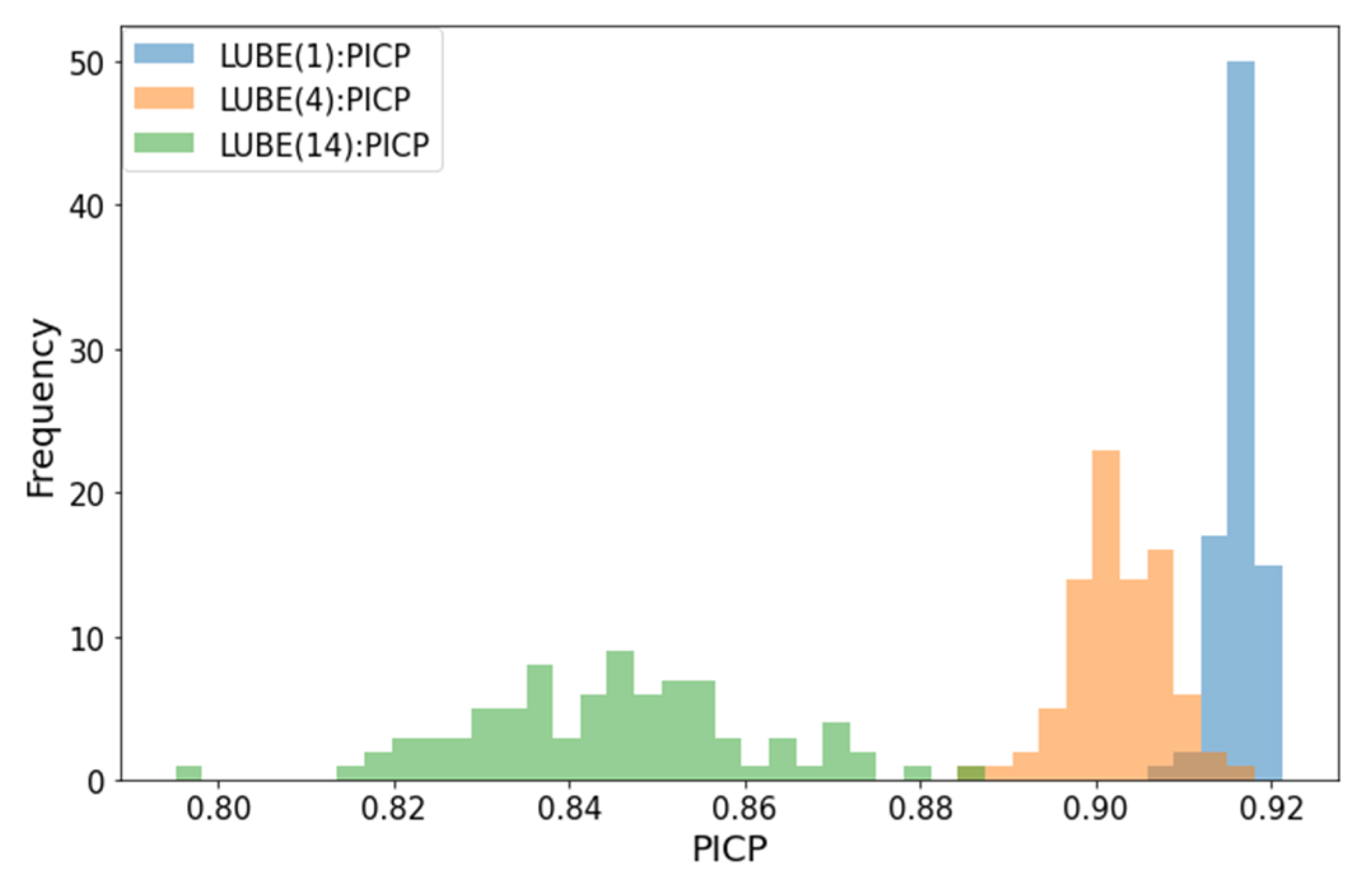
When features with high gain were selected, there was an improvement in the accuracy of PIs in both QR and LUBE compared to when all features were used. However, features with low gain rarely contribute to or worsen the accuracy of PIs. According to Loss, the low gain features reduced the accuracy of PIs in LUBE, especially when PV output fluctuations were large.

The remainder of the paper is organized as follows: Section 2 describes feature selection with RF. Section 3 describes LUBE. Section 4 evaluates the accuracy of PIs by LUBE and QR based on feature selection by RF. Section 5 concludes the study.

2. Feature Selection Using Random Forest

Because PV power output fluctuates due to weather factors, modeling accuracy varies greatly depending on the features used in the model. If features with additional variables that are effective in modeling are used, the modeling accuracy improves; otherwise, the modeling accuracy deteriorates. It also increases the complexity of the model and computational processing. In this study, feature selection was performed by RF, which is an ensemble model that is obtained by modeling a forecasting model that repeats binary classification on a tree called a “decision tree” for each of the multiple samples generated using the bootstrap method, and averaging the forecasting accuracy [29]. RF has been proved useful in forecasting renewable energy sources such as solar power and wind power, which are sensitive to environmental factors [30,31]. The conceptual diagram of feature selection by RF is shown in Figure 1 and the following procedure is used [32,33].

(i).

From the training data consisting of n sets of P predictors and corresponding target variables, n sets are extracted, allowing for overlap. The extraction is repeated to generate K bootstrap samples. When generating bootstrap samples, approximately two-thirds of the training data are extracted at least once from the sample and about one-third are never extracted. The group of samples that are not extracted is referred to as out-of-bag (OOB).

(ii).

A decision tree is modeled for each of the K bootstrap samples and the mean square error (MSE) is obtained using OOB as test data. ${\mathrm{MSE}}^{{\mathrm{OOB}}_{\mathrm{t}}}$ represents the MSE when ${\mathrm{OOB}}_{\mathrm{t}}$ is the test data. $Y$ is the target variable and the hat symbol represents the predicted value.

$${\mathrm{MSE}}^{{\mathrm{OOB}}_{\mathrm{t}}}=\frac{1}{n}{\displaystyle \sum }_{i=1}^n{\left|Y_i-\widehat{Y_{i,t}}\right|}^2$$

(1)

(iii).

One arbitrary feature from the OOB features is selected, randomly permuted, and the MSE is obtained again. This is repeated for all features.

$${\mathrm{MSE}}^{{\mathrm{OOB}}_{\mathrm{t}}}\left(X_{j}permuted\right)=\frac{1}{n}{\displaystyle \sum }_{i=1}^n{\left|Y_i-\widehat{Y_{i,t}}\left(X_{j}permuted\right)\right|}^2$$

(2)

where $X_j$ denotes the feature and $j=1, 2, \dots , \mathrm{P}$, ${\mathrm{MSE}}^{{\mathrm{OOB}}_{\mathrm{t}}}\left(X_{j}permuted\right)$ denotes the MSE at ${\mathrm{OOB}}_{\mathrm{t}}$ when the feature $X_j$ is permuted.

(iv).

The changes in MSE before and after permuting is obtained and the K results are averaged. Normalization is applied so that the sum of the importance of each feature is 1. If a feature is important to the accuracy of the forecast, permuting will significantly reduce the accuracy of the forecast. For unimportant features, the accuracy of the prediction is not affected.

$$\mathrm{MSE}dif\left(X_j\right)=\frac{1}{K}{\displaystyle \sum }_{t=1}^K\left({\mathrm{MSE}}^{{\mathrm{OOB}}_{\mathrm{t}}}\left(X_{j}permuted\right)-{\mathrm{MSE}}^{{\mathrm{OOB}}_{\mathrm{t}}}\right)$$

(3)

$$gain{X}_j=\frac{\mathrm{MSE}dif\left(X_j\right)}{{\sum }_{j=1}^P\mathrm{MSE}dif\left(X_j\right)}$$

(4)

3. Lower Upper Bound Estimation (LUBE)

LUBE is a nonparametric method that directly generates PIs using NNs with two outputs corresponding to the upper and lower bounds of the PIs [19]. Traditional methods such as the Delta and Bayesian methods are parametric methods that first perform point estimation and then generate PIs by assuming a distribution over the data [34,35]. LUBE directly generates PIs, which is simple, fast, and without special assumptions about the distribution or a large amount of computational work [21]. In LUBE, PIs are evaluated using the following three indicators. The conceptual diagram of the neural network in LUBE is shown in Figure 2.

3.1. Prediction Interval Coverage Probability (PICP)

PICP is an index that evaluates the percentage of measured values that fall within the interval of PIs and is one of the important evaluation indicators. The predicted lower and upper PI bounds are ${\widehat{y}}_{L_i}$, ${\widehat{y}}_{U_i}$. A vector, $\mathit{k}$, of length n represents whether each data point has been captured by the estimated PIs.

$$k_i=\left\{\begin{array}{c}1,if {\widehat{y}}_{L_i} \leqq y_i \leqq {\widehat{y}}_{U_i} \\ 0, else\hfill \end{array}\right.$$

(5)

We define the total number of data points captured as $c$.

$$c ≔{\displaystyle \sum }_{i=1}^n{k}_i$$

(6)

PICP is defined by Equation (7).

$$\mathrm{PICP} ≔\frac{\mathrm{c}}{n}$$

(7)

3.2. Mean Prediction Interval Width (MPIW)

MPIW represents the mean interval width and is an important metric for evaluating PIs; even if all measured values are within the interval and PICP is 100%, a too-wide MPIW implies high uncertainty and is meaningless as a forecast.

$$\mathrm{MPIW} ≔\frac{1}{\mathrm{c}}{\displaystyle \sum }_{i=1}^{\mathrm{n}}\left({\hat{\mathrm{y}}}_{U_i}-{\hat{\mathrm{y}}}_{L_i}\right)·k_i$$

(8)

3.3. Loss

The two key metrics, PICP and MPIW, need to be evaluated simultaneously when generating PIs using LUBE. However, if the width of PIs is narrowed, PICP is likely to decrease because some measured values will drop out of the PIs. In LUBE, the two trade-off indicators are evaluated simultaneously using Loss [28].

$$\mathrm{Loss}=\mathrm{MPIW}+\lambda \frac{n}{\alpha \left(1-\alpha \right)}max{\left(0,\left(1-\alpha \right)-\mathrm{PICP}\right)}^2$$

(9)

where $n$ is the number of data samples and α is a measure of the confidence level of the PIs. For example, when α = 0.05, 1 − α is 95%. At this time, the qualitative understanding in the equation is that if PICP does not exceed 0.95, a penalty is imposed by λ. In this case, Loss is the sum of MPIW, and the PICP term including λ. λ is the parameter that imposes a penalty and, at the same time, a tuning parameter that relates MPIW to PICP. If it exceeds 0.95, Loss is equal to MPIW. In PIs, when PICP is much lower than the established confidence level, the PIs can be considered lacking validity [14]. Therefore, in determining λ, there is need to adjust PICP and then consider the combination with MPIW.

3.4. Continuous Ranked Probability Score (CRPS)

In LUBE, the neural network learns to minimize Loss. Since the ratio of PICP and MPIW changes depending on the value of λ in Loss, the evaluation of PIs was also performed using CRPS [36]. The CRPS measures the difference between the predicted and observed cumulative distribution functions and is expressed by

$$crps\left(F,y\right)={{\displaystyle \int }}_{-\infty }^{\infty }{\left[F\left(t\right)-H\left(t-y\right)\right]}^2 dt$$

(10)

$$\mathrm{CRPS}=\frac{1}{n}{\displaystyle \sum }_{i=1}^{n}crps\left(F_i,y_i\right)$$

(11)

where $F$ is the predictive cumulative distribution function (CDF) and y is the verifying observation, $H\left(t-y\right)$ denotes the Heaviside function and takes the value 0 when $t<y$ and the value 1 otherwise, and n is total points.

In Equation (11), when $F$ follows a Gaussian distribution with mean $\mu$ and dispersion ${\sigma }^2$, it is expressed by

$$crps\left[N\left(\mu ,{\sigma }^2\right),y\right]= \sigma \{\frac{y-\mu }{\sigma }\left[2\Phi \left(\frac{y-\mu }{\sigma }\right)-1\right]+2\phi \left(\frac{y-\mu }{\sigma }\right)-\frac{1}{\sqrt{\pi }}\}$$

(12)

where $\phi \left(\frac{y-\mu }{\sigma }\right)$ and $\Phi \left(\frac{y-\mu }{\sigma }\right)$ denote probability density functions (PDF) and the CDF, respectively, of the normal distribution with mean 0 and variance 1 evaluated at the normalized prediction error. To calculate the (12) expression in LUBE, we used proper scoring [37], an external python library. G. Mitrentsis et al. [18] used proper scoring to calculate CRPS for LUBE. However, since LUBE outputs PIs directly without assuming a distribution, care must be taken when evaluating calculations assuming a Gaussian distribution.

4. Case Study

For the probabilistic modeling of solar power generation, excluding unnecessary features improves modeling accuracy, but missing necessary features reduces modeling accuracy. In particular, PV modeling is difficult when output fluctuation is large, and if unnecessary features are included, the modeling accuracy is likely to be even lower. In this case study, we evaluated the importance of each feature for the probabilistic modeling. We first used RF to evaluate the gain of 14 features, consisting of weather and time-oriented features, for modeling PV power output. Next, PIs were generated using LUBE with a confidence level of 95%. In LUBE, we used 14 pairs of features added in order from variables with the highest gain. The 2-week average modeling accuracy of the PIs from each feature was evaluated, and the optimal features were considered. We also compared PIs by QR using the gradient boosted regression trees method with those of LUBE. See L. Massidda’s study [38] for details on the principle of QR. We also evaluated the robustness of the modeling by setting the number of simulations to 85 in LUBE. Finally, in relation to output fluctuation, we considered each day to evaluate when modeling was successful and when they failed, with and without feature selection.

The PV power plant subject of this study is in Tokyo, Japan, and has a capacity of 14.7 kW. PV power generation is observed every 30 min for 24 h. In addition to power generation data, atmospheric temperature, precipitation, degree of cloudiness, solar radiation, wind speed, and humidity were obtained from nearby meteorological observatories. The corresponding year, month, day, and hour were also added to the data set. The time data were expressed as a trigonometric function to account for periodicity. For example, the trigonometric representation of hour considers 24 h as one cycle, and daily considers the number of days in a month as one cycle. Azimuth, zenith, and declination [39] are also considered effective features, but are not included in this study. All features were standardized for uniformity of scale. Figure 3 shows how the data is divided. The observed data are for the period from 15 August 2013 to 14 June 2014. The feature selection by RF used data from 15 August 2013 to 31 May 2014. Training data for PIs generation by the LUBE and QR used data from 15 August 2013 to 16 May 2014. Validation data were from 17 May 2014 to 31 May 2014, and test data were from 1 June 2014 to 14 June 2014. Add data were from 1 June 2014 to the day before the test day. Adding the most recent data to the training and validation data was expected to improve modeling accuracy. Figure 4 shows a flowchart of LUBE using feature selection by random forest. We used NN consisting of an input layer, an intermediate layer with 100 neurons, and an output layer in LUBE. Regarding the NN parameters, from the combinations of nλ included in Equation (9), learning rate, and epochs listed in

Table 1. Grid search for neural network and quantile regression.

Model	Parameter	Search Values	Selected Value
LUBE	nλ	3, 5, 7	5
	learning rate	0.01, 0.001, 0.0001	0.001
	epochs	100, 500, 1000, 3000	3000
QR	learning rate	0.05, 0.02, 0.01	0.05
	maximum depth of trees	3, 4, 5	3
	minimum number of samples in leaf	3, 5, 7	7
	number of estimates	100, 200, 500	500

, the parameters with high PICP and narrow MPIW were adopted when all features were used. In QR, a grid search was performed from the parameters of Table 1 so that the CRPS would be small.

4.1. Result of the Feature Selection by Random Forest

Table 2. Evaluating the importance of features using random forest.

Feature	Gain	Feature	Gain
solar radiation	0.7644	atmospheric temperature	0.0065
hour sine	0.0961	monthly cosine	0.0062
hour cosine	0.0757	wind speed	0.0057
annual cosine	0.0130	daily sine	0.0038
degree of cloudiness	0.0076	daily cosine	0.0037
annual sine	0.0069	monthly sine	0.0025
humidity	0.0069	precipitation	0.0003

shows the results of feature selection using RF. The gain for solar radiation is 0.764, indicating that it is an extremely important feature. The hour sine and hour cosine have a combined gain of 0.172, and the annual cosine has a gain of 0.013. The gains for the other features are almost zero, indicating that they are of low importance.

4.2. Prediction Intervals by Lower Upper Boundary Estimation and Quantile Regression

4.2.1. Evaluation of Prediction Intervals at 2-Week Average

Figure 5 shows the correspondence between the number of features and the two-week average of Loss in LUBE and total gain. In Figure 5, the green triangle means median, and the small circle means outliers. LUBE(1) includes only the solar radiation, which is the highest gain. LUBE(4) includes solar radiation, hour sine, hour cosine, and annual cosine. LUBE(14) includes all features. The same applies to QR(1), (4), (14), etc.

Table 3. Statistics of 2-week average Loss.

Number of Features	Min	Max	Mean	Median	Standard Deviation
LUBE(1)	2.28	2.37	2.32	2.32	0.0193
LUBE(4)	1.95	2.30	2.13	2.13	0.0861
LUBE(14)	2.65	6.03	3.74	3.70	0.5967

shows the Loss statistics for LUBE(1), (4), and (14). Figure 6 shows a histogram of the results of 85 simulations of Loss for the 2-week average of LUBE(1), (4), and (14).

Figure 5 shows that features with a gain of nearly zero act as noise, reducing the accuracy and robustness of the modeling in LUBE. LUBE(4) has the smallest Loss, increases thereafter, and at LUBE(14) has the largest. The distribution of Loss in the box-and-whisker diagram is expanding from LUBE(4) to LUBE(14). To evaluate the modeling accuracy and robustness, we compared LUBE(14) with LUBE(1), which includes only solar radiation, and LUBE(4), which has the lowest Loss. In Table 3, LUBE(14) is significantly worse than LUBE(1) and LUBE(4) in all statistics. At the median, Loss is 1.38 kW greater than LUBE(1) and 1.57 kW greater than LUBE(4). In addition, as shown by the standard deviations in Table 3 and histograms in Figure 6, the distribution of LUBE(14) is wide, and the modeling accuracy is varied. These results indicate that features that are low in gain should be removed because they reduce not only modeling accuracy but also robustness.

We then similarly evaluated PICP and MPIW. Figure 7 and Figure 8 show the 2-week average PICP and MPIW in LUBE and QR, respectively. In Figure 7 and Figure 8, the green triangle means median, and the small circle means outliers.

Table 4. Statistics of 2-week average PICP.

Number of Features	Min	Max	Mean	Median	Standard Deviation
LUBE(1)	0.907	0.921	0.916	0.917	0.00231
LUBE(4)	0.886	0.916	0.903	0.902	0.00537
LUBE(14)	0.795	0.886	0.845	0.845	0.0160
QR(2)	-	-	-	0.942	-

and

Table 5. Statistics of 2-week average MPIW.

Number of Features	Min	Max	Mean	Median	Standard Deviation
LUBE(1)	2.02	2.13	2.07	2.07	0.0151
LUBE(4)	1.47	1.66	1.53	1.53	0.0340
LUBE(14)	1.53	1.78	1.64	1.65	0.0536
QR(2)	-	-	-	2.51	-

show the PICP and MPIW statistics for LUBE(1), (4), (14), and QR(2), respectively; Figure 9 and Figure 10 show the histograms for LUBE(1), (4), and (14).

Figure 7 and Figure 8 show that the features after LUBE(4) work as noise in LUBE, because the PICP tends to decrease and MPIW tends to increase after LUBE(4). In QR, they also show features after QR(4) do not contribute to the prediction accuracy, because there is almost no change in PICP and MPIW after QR(4). Compared to LUBE, QR has wider MPIW and higher PICP. In Table 4 and Table 5, we evaluated the impact of features in LUBE. In Table 4, comparing median values, PICP is 0.072 and 0.057 higher for LUBE(1), and LUBE(4), respectively, compared to LUBE(14). In Table 5, MPIW is 0.12 kW narrower for LUBE(4) than for LUBE(14). However, in LUBE(1), MPIW is 0.42 kW wider than in LUBE(14). This means that LUBE(1) is highly uncertain because it contains only one feature. LUBE(4) is the narrowest MPIW in Table 5 because it contains enough features with high gain. Therefore, LUBE(4) outperforms LUBE(14) in MPIW and PICP as well. From the standard deviations in Table 4 and Table 5 and the histograms in Figure 9 and Figure 10, PICP and MPIW, as well as Loss, features with low gain reduce the robustness of the modeling. These results indicate that in PICP and MPIW, as in Loss, the features after LUBE(4) are noise.

Finally, using CRPS, we evaluated LUBE and QR. Figure 11 shows the correspondence between the number of features and the two-week average of CRPS in LUBE and QR, and total gain. In Figure 11, the green triangle means median, and the small circle means outliers.

Table 6. Statistics of 2-week average CRPS.

Number of Features	Min	Max	Mean	Median	Standard Deviation
LUBE(1)	0.53	0.54	0.53	0.53	0.0024
LUBE(4)	0.39	0.43	0.41	0.41	0.0056
LUBE(14)	0.42	0.46	0.44	0.44	0.0064
QR(2)	-	-	-	0.51	-

shows the statistics of CRPS for the 2-week average of LUBE(1), (4), (14) and QR(2).

Figure 11 shows that both LUBE(1) and QR(1) have poor modeling accuracy because they only include solar radiation as a feature. In Figure 11, the CRPS after LUBE(4) and QR(4) is almost constant, indicating that features with low gain do not contribute to modeling accuracy. LUBE has the smallest CRPS in LUBE(4). However, QR has the smallest CRPS in QR(2), not QR(4). This is because QR has PICP close to 95% for any number of features in Figure 7, and QR(2) has the narrowest MPIW in Figure 8. Therefore, we can conclude that QR(2) and LUBE(4) use enough features as needed and have high modeling accuracy, and features with low gain do not contribute to improving modeling accuracy.

4.2.2. Accuracy Evaluation by Forecast Target Date

To evaluate the relationship between output fluctuation and modeling accuracy according to features, we analyze LUBE(14), which includes all features, LUBE(1), LUBE(4), and QR(2) by day as shown in

Table 7. Evaluation for LUBE(1), (4), (14) and QR(2) by PICP and MPIW from 1 June to 14 June.

		PICP				MPIW [kW]
Day	Fluctuation [kW]	LUBE(1)	LUBE(4)	LUBE(14)	QR(2)	LUBE(1)	LUBE(4)	LUBE(14)	QR(2)
1	0.489	0.958	0.979	0.979	0.938	2.45	1.55	2.02	2.91
2	0.582	0.896	0.864	0.791	0.958	2.50	1.52	1.40	3.01
3	0.505	0.916	0.875	0.831	1.000	2.50	1.61	1.58	2.88
4	0.522	0.895	0.853	0.834	0.938	2.41	1.49	1.59	2.86
5	0.350	0.979	0.979	0.979	1.000	1.74	1.66	2.03	2.13
6	0.193	0.916	0.984	0.911	1.000	0.85	1.44	1.61	1.48
7	0.233	0.937	0.984	1.000	1.000	1.25	1.46	1.92	1.86
8	0.412	0.894	0.917	0.875	0.896	1.64	1.65	1.50	2.25
9	0.968	0.874	0.833	0.765	0.875	2.73	1.63	1.47	2.90
10	0.909	0.835	0.849	0.815	0.938	2.53	1.63	1.66	2.86
11	0.308	0.957	0.879	0.876	0.875	1.43	1.10	1.44	1.69
12	0.271	0.937	0.956	0.958	0.958	1.92	1.58	1.76	2.34
13	0.807	0.894	0.808	0.739	0.896	2.56	1.36	1.53	3.03
14	0.513	0.937	0.974	0.937	0.917	2.43	1.60	1.68	2.90
Average (Fluctuation > 0.5 kW)	0.687	0.892	0.865	0.816	0.932	2.52	1.55	1.56	2.92
Average (Fluctuation < 0.5 kW)	0.322	0.940	0.954	0.940	0.952	1.61	1.49	1.75	2.09
Average (All days)	0.504	0.916	0.910	0.878	0.942	2.07	1.52	1.66	2.51

and

Table 8. Evaluation for LUBE (1), (4), (14) and QR (2) by Loss and CRPS from June 1 to 14.

		Loss [kW]			CRPS [kW]
Day	Fluctuation [kW]	LUBE(1)	LUBE(4)	LUBE(14)	LUBE(1)	LUBE(4)	LUBE(14)	QR(2)
1	0.489	2.45	1.55	2.02	0.62	0.26	0.27	0.63
2	0.582	2.81	2.30	4.05	0.75	0.48	0.49	0.55
3	0.505	2.62	2.21	3.07	0.58	0.48	0.53	0.43
4	0.522	2.73	2.49	3.00	0.61	0.45	0.47	0.38
5	0.350	1.74	1.66	2.03	0.26	0.26	0.31	0.31
6	0.193	0.97	1.44	1.77	0.20	0.20	0.22	0.28
7	0.233	1.27	1.46	1.92	0.20	0.15	0.22	0.30
8	0.412	1.96	1.76	2.09	0.38	0.35	0.41	0.40
9	0.968	3.33	3.08	5.07	0.87	0.64	0.70	0.70
10	0.909	3.93	2.70	3.57	0.91	0.69	0.72	0.73
11	0.308	1.43	1.64	2.01	0.29	0.42	0.44	0.51
12	0.271	1.93	1.58	1.76	0.31	0.24	0.24	0.36
13	0.807	2.89	3.50	6.22	0.87	0.73	0.76	0.89
14	0.513	2.45	1.60	1.69	0.62	0.28	0.29	0.73
Average (Fluctuation > 0.5 kW)	0.687	2.97	2.55	3.81	0.74	0.54	0.57	0.63
Average (Fluctuation < 0.5 kW)	0.322	1.68	1.58	1.94	0.32	0.27	0.30	0.40
Average (All days)	0.504	2.32	2.07	2.88	0.53	0.40	0.43	0.51

. In Table 7 and Table 8, out of 85 simulations in LUBE, the median of Loss and corresponding MPIW, PICP, and CRPS for each day are shown. In Table 7 and Table 8, we evaluated the modeling accuracy using an index named Fluctuation, which is the average output fluctuations at 30-min intervals over a day. This study defines Fluctuation as indicated in Equation (13).

$$\mathrm{Fluctuation}=\frac{{\sum }_{i=1}^{48}\left|v\left(t_i\right)-v\left(t_{i-1}\right)\right|}{48}$$

(13)

where $v\left(t_i\right)$ represents the power output at time $t_i$. Since output power is observed at 30-min intervals, there are 48 i in a day. For example, when Fluctuation is 0 kW, the daily generation output is constant. In Table 7 and Table 8, the threshold for Fluctuation is 0.5 kW, which is the average of the output fluctuations for all days, and days when the output fluctuations exceed 0.5 kW are highlighted in gray. On each day, the highest PICP and the lowest MPIW, Loss, and CRPS are shown in bold among LUBE(1), (4), (14), and QR(2). For example, on 2 June, Fluctuation is 0.582 kW, QR(2) has the highest PICP of 0.958 and LUBE(14) has the narrowest MPIW of 1.40 kW. LUBE(4) has the lowest Loss and CRPS at 2.30 kW and 0.48 kW, respectively.

Table 9. Correlation coefficient with 30-min output fluctuation for LUBE (1), (4), (14), and QR (2).

Metric	PICP				MPIW
Method	LUBE(1)	LUBE(4)	LUBE(14)	QR(2)	LUBE(1)	LUBE (4)	LUBE(14)	QR(2)
Correlation coefficient	−0.726	−0.758	−0.762	−0.51	0.818	0.258	−0.355	0.862
Metric	Loss				CRPS
Method	LUBE(2)	LUBE(4)	LUBE(14)	QR(2)	LUBE(1)	LUBE(4)	LUBE(14)	QR(2)
Correlation coefficient	0.932	0.879	0.821	-	0.949	0.894	0.891	0.807

shows the correlation coefficients between output fluctuations at 30-min intervals and PICP, MPIW, Loss, and CRPS for LUBE(1), (4), (14), and QR(2).

Based on the strong correlation between Loss, CRPS and 30-min output fluctuation for all methods in Table 9, it is easy to be modeling when the output fluctuation is small and difficult when it is large. When Fluctuation does not exceed 0.5 kW in Table 7 and Table 8, LUBE(4) is the best. From Average (Fluctuation < 0.5 kW) in Table 7 and Table 8, PICP, MPIW, Loss, and CRPS over 7 days is best for LUBE(4). When Fluctuation exceeds 0.5 kW, LUBE(4) or QR(2) is suitable for modeling. As indicated by the strong correlation between MPIW and output fluctuation for QR(2) in Table 9, QR(2) has a wide MPIW and high uncertainty on days when Fluctuation is large. However, PIs in QR(2) include many real values and have the largest average PICP in Table 7. In Table 8 Average (Fluctuation > 0.5 kW), CRPS is smallest for LUBE(4), but there are several days when it is more than 0.1 below the confidence level; if the PICP is much below the confidence level, the PIs are not considered valid, so LUBE(4) or QR(2) is appropriate for modeling. Throughout the 14 days, the CRPS and Loss of LUBE (14) are larger than LUBE (4) on all days. In particular, according to Loss, features with low gain on days with large output fluctuation act as noise in LUBE. Therefore, we can conclude that features with low gain should not be used.

4.2.3. Days of Maximum and Minimum Output Fluctuation

Figure 12a shows the PIs for LUBE(1), (4), (14) and QR (2) for the day with the lowest Fluctuation of 0.193 kW in Table 7 and Table 8. PICP is above 0.9 in all methods in Table 7. LUBE(1) has the smallest MPIW and Loss, and LUBE(4) is second in Table 7 and Table 8. CRPS is the smallest for LUBE(1), (4) in Table 8. Therefore, LUBE(1) is appropriate, followed by LUBE(4).

Figure 12b shows the PIs for LUBE(1), (4), (14) and QR (2) for the day with the largest Fluctuation of 0.968 kW in Table 7 and Table 8. LUBE(1) or QR (2) is best for 9 June. CRPS is the smallest in LUBE(4). However, PICP of LUBE(4) is 0.833, which is more than 0.1 below the confidence level. The CRPS of LUBE(1) and QR(2) is 0.70, the second smallest, and the PICP is about 0.875. Therefore, LUBE(1) or QR(2) is best.

5. Conclusions

The objective of this study was to improve the PICP, MPIW, Loss, and CRPS of PIs using LUBE and QR by removing unnecessary features. We considered the change in PI accuracy by incorporating, in order, the features with high gain evaluated by RF into the features used for LUBE and QR. In the number of features 1, which includes only solar radiation evaluated as the most important feature, there was high uncertainty and wide MPIW, high PICP, and large CRPS in LUBE and QR. In the number of features 14 without feature selection, features with a gain of nearly zero led to a decrease in the accuracy of PIs in LUBE and QR. In particular, according to Loss, features with low gain on days with large output fluctuation act as noise in LUBE. In QR, the number of features 2, which includes solar radiation and hour sine, and in LUBE, the number of features 4, which adds hour cosine and annual cosine to the above two features, contained enough features as needed and had the lowest CRPS and Loss. In LUBE, the number of features 4 improved Loss by 1.57 kW, CRPS by 0.03 kW, PICP by 0.057, and MPIW by 0.12 kW compared to the number of features 14 on a 14.7 kW PV system. However, on days with large output fluctuations, there are days when the PICP is more than 0.1 lower than the confidence level in LUBE. Therefore, the challenge remains to generate PIs with PICP close to the confidence level even on days with strong fluctuations.

References

1. Ahmed, R.; Sreeram, V.; Mishra, Y.; Arif, M.D. A Review and Evaluation of the State-of-the-Art in PV Solar Power Forecasting: Techniques and Optimization. Renew. Sustain. Energy Rev. 2020, 124, 109792. [Google Scholar] [CrossRef]
2. Kodaira, D.; Jung, W.; Han, S. Optimal Energy Storage System Operation for Peak Reduction in a Distribution Network Using a Prediction Interval. IEEE Trans. Smart Grid 2020, 11, 2208–2217. [Google Scholar] [CrossRef]
3. Rowe, M.; Yunusov, T.; Haben, S.; Singleton, C.; Holderbaum, W.; Potter, B. A Peak Reduction Scheduling Algorithm for Storage Devices on the Low Voltage Network. IEEE Trans. Smart Grid 2014, 5, 2115–2124. [Google Scholar] [CrossRef]
4. Hafiz, F.; Awal, M.A.; De Queiroz, A.R.; Husain, I. Real-Time Stochastic Optimization of Energy Storage Management Using Deep Learning-Based Forecasts for Residential PV Applications. IEEE Trans. Ind. Appl. 2020, 56, 2216–2226. [Google Scholar] [CrossRef]
5. Dolara, A.; Leva, S.; Manzolini, G. Comparison of Different Physical Models for PV Power Output Prediction. Sol. Energy 2015, 119, 83–99. [Google Scholar] [CrossRef] [Green Version]
6. Miyazaki, Y.; Kameda, Y.; Kondoh, J. A Power-Forecasting Method for Geographically Distributed PV Power Systems Using Their Previous Datasets. Energies 2019, 12, 4815. [Google Scholar] [CrossRef] [Green Version]
7. Saint-Drenan, Y.M.; Good, G.H.; Braun, M. A Probabilistic Approach to the Estimation of Regional Photovoltaic Power Production. Sol. Energy 2017, 147, 257–276. [Google Scholar] [CrossRef] [Green Version]
8. Huang, R.; Huang, T.; Gadh, R.; Li, N. Solar Generation Prediction Using the ARMA Model in a Laboratory-Level Micro-Grid. In Proceedings of the 2012 IEEE 3rd International Conference on Smart Grid Communications, SmartGridComm 2012, Tainan, Taiwan, 5–8 November 2012; pp. 528–533. [Google Scholar]
9. Liu, J.; Fang, W.; Zhang, X.; Yang, C. An Improved Photovoltaic Power Forecasting Model with the Assistance of Aerosol Index Data. IEEE Trans. Sustain. Energy 2015, 6, 434–442. [Google Scholar] [CrossRef]
10. Theocharides, S.; Theristis, M.; Makrides, G.; Kynigos, M.; Spanias, C.; Georghiou, G.E. Comparative Analysis of Machine Learning Models for Day-Ahead Photovoltaic Power Production Forecasting. Energies 2021, 14, 1081. [Google Scholar] [CrossRef]
11. Jang, H.S.; Bae, K.Y.; Park, H.S.; Sung, D.K. Solar Power Prediction Based on Satellite Images and Support Vector Machine. IEEE Trans. Sustain. Energy 2016, 7, 1255–1263. [Google Scholar] [CrossRef]
12. Tao, C.; Lu, J.; Lang, J.; Peng, X.; Cheng, K.; Duan, S. Short-Term Forecasting of Photovoltaic Power Generation Based on Feature Selection and Bias Compensation–Lstm Network. Energies 2021, 14, 3086. [Google Scholar] [CrossRef]
13. Generations, P.; Kodaira, D.; Tsukazaki, K.; Kure, T.; Kondoh, J. Improving Forecast Reliability for Geographically Distributed. Energies 2021, 14, 7340. [Google Scholar]
14. Yang, H.T.; Huang, C.M.; Huang, Y.C.; Pai, Y.S. A Weather-Based Hybrid Method for 1-Day Ahead Hourly Forecasting of PV Power Output. IEEE Trans. Sustain. Energy 2014, 5, 917–926. [Google Scholar] [CrossRef]
15. Sheng, H.; Xiao, J.; Cheng, Y.; Ni, Q.; Wang, S. Short-Term Solar Power Forecasting Based on Weighted Gaussian Process Regression. IEEE Trans. Ind. Electron. 2018, 65, 300–308. [Google Scholar] [CrossRef]
16. Agoua, X.G.; Girard, R.; Kariniotakis, G. Probabilistic Models for Spatio-Temporal Photovoltaic Power Forecasting. IEEE Trans. Sustain. Energy 2019, 10, 780–789. [Google Scholar] [CrossRef] [Green Version]
17. Almeida, M.P.; Muñoz, M.; de la Parra, I.; Perpiñán, O. Comparative Study of PV Power Forecast Using Parametric and Nonparametric PV Models. Sol. Energy 2017, 155, 854–866. [Google Scholar] [CrossRef] [Green Version]
18. Mitrentsis, G.; Lens, H. An Interpretable Probabilistic Model for Short-Term Solar Power Forecasting Using Natural Gradient Boosting. Appl. Energy 2022, 309, 118473. [Google Scholar] [CrossRef]
19. Khosravi, A.; Nahavandi, S.; Creighton, D.; Atiya, A.F. Lower Upper Bound Estimation Method for Construction of Neural Network-Based Prediction Intervals. IEEE Trans. Neural Netw. 2011, 22, 337–346. [Google Scholar] [CrossRef]
20. Khosravi, A.; Nahavandi, S.; Creighton, D. Prediction Intervals for Short-Term Wind Farm Power Generation Forecasts. IEEE Trans. Sustain. Energy 2013, 4, 602–610. [Google Scholar] [CrossRef]
21. Quan, H.; Srinivasan, D.; Khosravi, A. Uncertainty Handling Using Neural Network-Based Prediction Intervals for Electrical Load Forecasting. Energy 2014, 73, 916–925. [Google Scholar] [CrossRef]
22. Ni, Q.; Zhuang, S.; Sheng, H.; Kang, G.; Xiao, J. An Ensemble Prediction Intervals Approach for Short-Term PV Power Forecasting. Sol. Energy 2017, 155, 1072–1083. [Google Scholar] [CrossRef]
23. Raza, M.Q.; Nadarajah, M.; Ekanayake, C. On Recent Advances in PV Output Power Forecast. Sol. Energy 2016, 136, 125–144. [Google Scholar] [CrossRef]
24. De Giorgi, M.G.; Congedo, P.M.; Malvoni, M. Photovoltaic Power Forecasting Using Statistical Methods: Impact of Weather Data. IET Sci. Meas. Technol. 2014, 8, 90–97. [Google Scholar] [CrossRef]
25. Zhong, Y.J.; Wu, Y.K. Short-Term Solar Power Forecasts Considering Various Weather Variables. In Proceedings of the 2020 International Symposium on Computer, Consumer and Control, IS3C 2020, Taichung City, Taiwan, 13–16 November 2020; Institute of Electrical and Electronics Engineers Inc.: Piscataway, NJ, USA, 2020; pp. 432–435. [Google Scholar]
26. Lundberg, S.M.; Erion, G.; Chen, H.; DeGrave, A.; Prutkin, J.M.; Nair, B.; Katz, R.; Himmelfarb, J.; Bansal, N.; Lee, S.-I. From Local Explanations to Global Understanding with Explainable AI for Trees. Nat. Mach. Intell. 2020, 2, 56–67. [Google Scholar] [CrossRef] [PubMed]
27. Lauret, P.; David, M.; Pinson, P. Verification of Solar Irradiance Probabilistic Forecasts. Sol. Energy 2019, 194, 254–271. [Google Scholar] [CrossRef] [Green Version]
28. Pearce, T.; Zaki, M.; Brintrup, A.; Neely, A. High-Quality Prediction Intervals for Deep Learning: A Distribution-Free, Ensembled Approach. In Proceedings of the 35th International Conference on Machine Learning, Stockholm, Sweden, 10–15 July 2018; Volume 9, pp. 6473–6482. [Google Scholar]
29. Breiman, L. Random Forests; Springer: Berlin/Heidelberg, Germany, 2001; Volume 45. [Google Scholar]
30. Kim, S.G.; Jung, J.Y.; Sim, M.K. A Two-Step Approach to Solar Power Generation Prediction Based on Weather Data Using Machine Learning. Sustainability 2019, 11, 1501. [Google Scholar] [CrossRef] [Green Version]
31. Lahouar, A.; Ben Hadj Slama, J. Hour-Ahead Wind Power Forecast Based on Random Forests. Renew. Energy 2017, 109, 529–541. [Google Scholar] [CrossRef]
32. Grömping, U. Variable Importance Assessment in Regression: Linear Regression versus Random Forest. Am. Stat. 2009, 63, 308–319. [Google Scholar] [CrossRef]
33. Svetnik, V.; Liaw, A.; Tong, C.; Christopher Culberson, J.; Sheridan, R.P.; Feuston, B.P. Random Forest: A Classification and Regression Tool for Compound Classification and QSAR Modeling. J. Chem. Inf. Comput. Sci. 2003, 43, 1947–1958. [Google Scholar] [CrossRef]
34. Khosravi, A.; Nahavandi, S.; Creighton, D.; Atiya, A.F. Comprehensive Review of Neural Network-Based Prediction Intervals and New Advances. IEEE Trans. Neural Netw. 2011, 22, 1341–1356. [Google Scholar] [CrossRef]
35. Panamtash, H.; Zhou, Q.; Hong, T.; Qu, Z.; Davis, K.O. A Copula-Based Bayesian Method for Probabilistic Solar Power Forecasting. Sol. Energy 2020, 196, 336–345. [Google Scholar] [CrossRef]
36. Gneiting, T.; Raftery, A.E.; Westveld, A.H.; Goldman, T. Calibrated Probabilistic Forecasting Using Ensemble Model Output Statistics and Minimum CRPS Estimation. Mon. Weather. Rev. 2005, 133, 1098–1118. [Google Scholar] [CrossRef]
37. Stephan Hoyer Properscoring. Available online: https://github.com/TheClimateCorporation/properscoring.git (accessed on 17 May 2022).
38. Massidda, L.; Marrocu, M. Quantile Regression Post-Processing Ofweather Forecast for Short-Term Solar Power Probabilistic Forecasting. Energies 2018, 11, 1763. [Google Scholar] [CrossRef] [Green Version]
39. Markovics, D.; Mayer, M.J. Comparison of Machine Learning Methods for Photovoltaic Power Forecasting Based on Numerical Weather Prediction. Renew. Sustain. Energy Rev. 2022, 161, 112364. [Google Scholar] [CrossRef]
Figure 1. Feature selection by RF.
Energies 15 05337 g001
Figure 2. LUBE.
Energies 15 05337 g002
Figure 3. Lower upper bound estimation method with random forest.
Energies 15 05337 g003
Figure 4. Flowchart of LUBE with feature selection by random forest.
Energies 15 05337 g004
Figure 5. Number of features, 2-week average Loss in LUBE, and total gain.
Energies 15 05337 g005
Figure 6. Histograms of 2-week average Loss for LUBE(1), (4), and (14).
Energies 15 05337 g006
Figure 7. Number of features and 2-week average PICP in LUBE and QR.
Energies 15 05337 g007
Figure 8. Number of features and 2-week average MPIW in LUBE and QR.
Energies 15 05337 g008
Figure 9. Histograms of 2-week average PICP for LUBE (1), (4), and (14).
Energies 15 05337 g009
Figure 10. Histograms of 2-week average MPIW for LUBE(1), (4), and (14).
Energies 15 05337 g010
Figure 11. Number of features, 2-week average CRPS in LUBE and QR, and total gain.
Energies 15 05337 g011
Figure 12. Prediction intervals for LUBE(1), (4), (14), and QR(2): (a) 6 June, the day with the smallest output fluctuation in two weeks.; (b) 9 June, the day of the largest output fluctuation in two weeks.
Energies 15 05337 g012