
A Gas Concentration Prediction Method Driven by a Spark Streaming Framework


Abstract
:1. Introduction
2. Materials and Methods
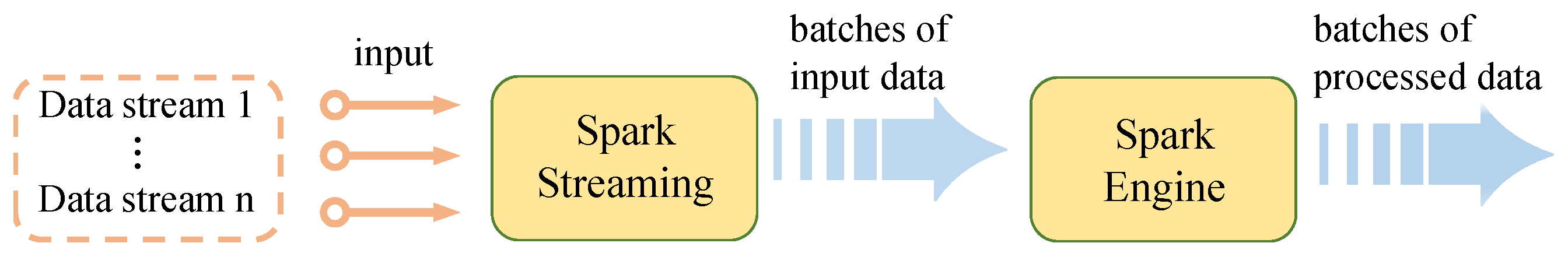
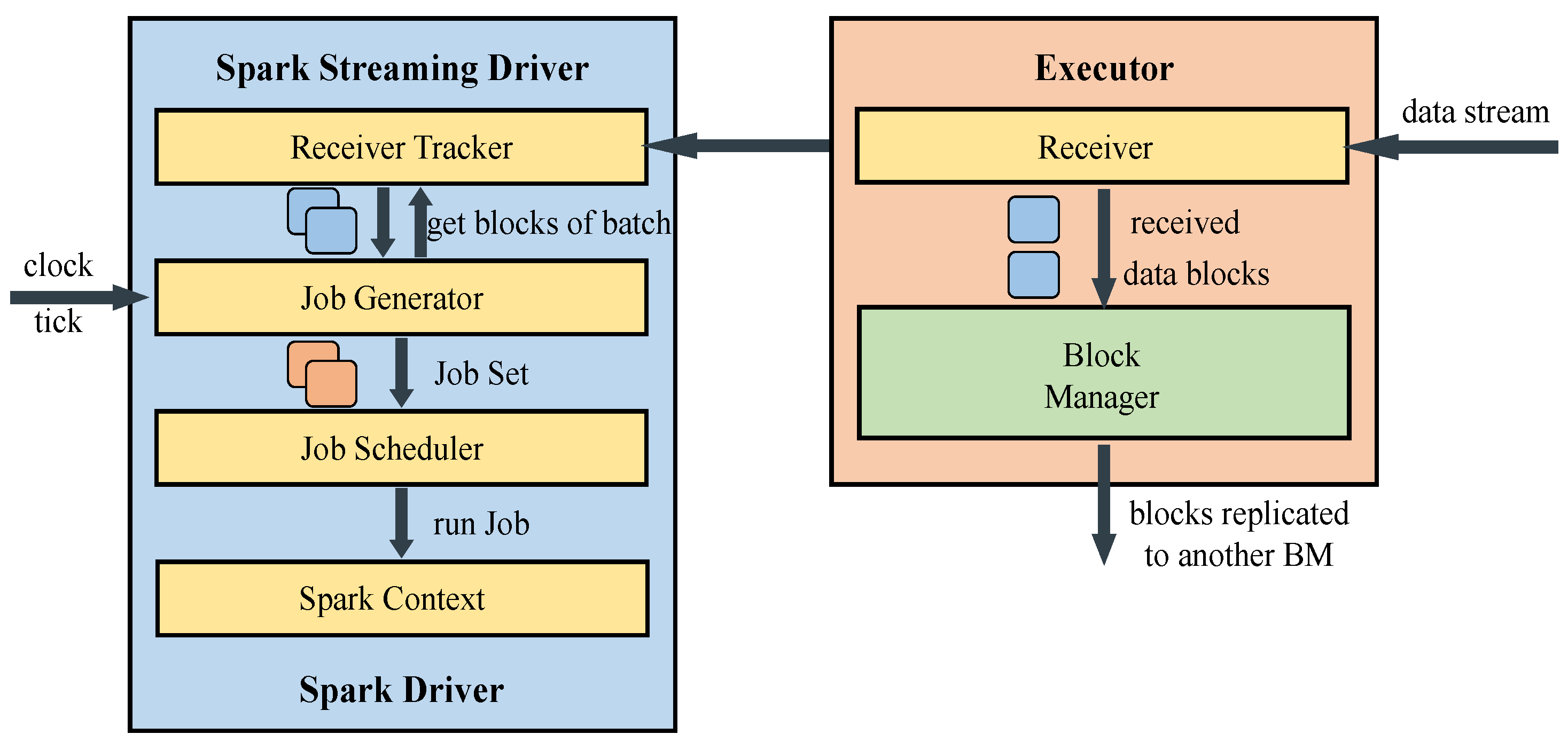
2.1. Spark Streaming Framework
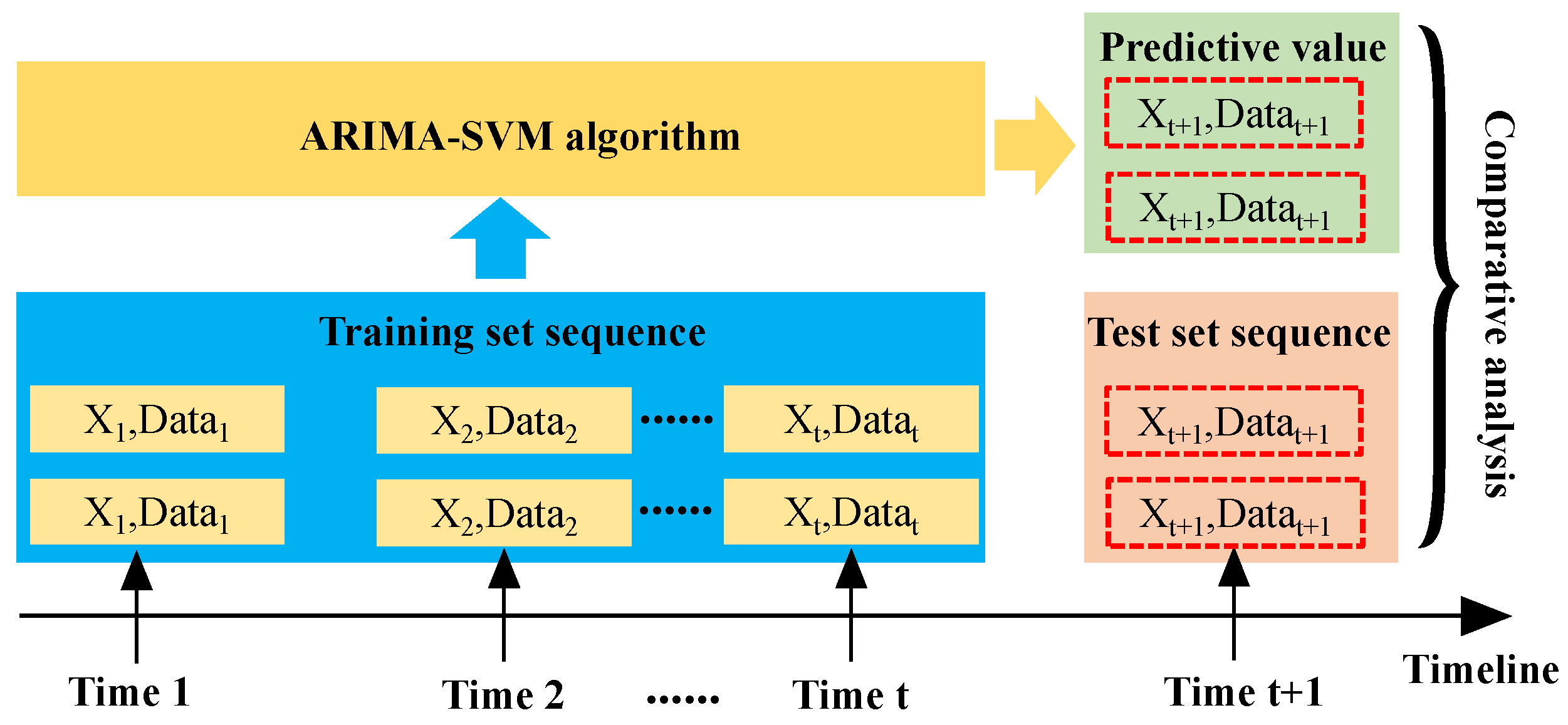
2.2. ARIMA-SVM Gas Prediction Model
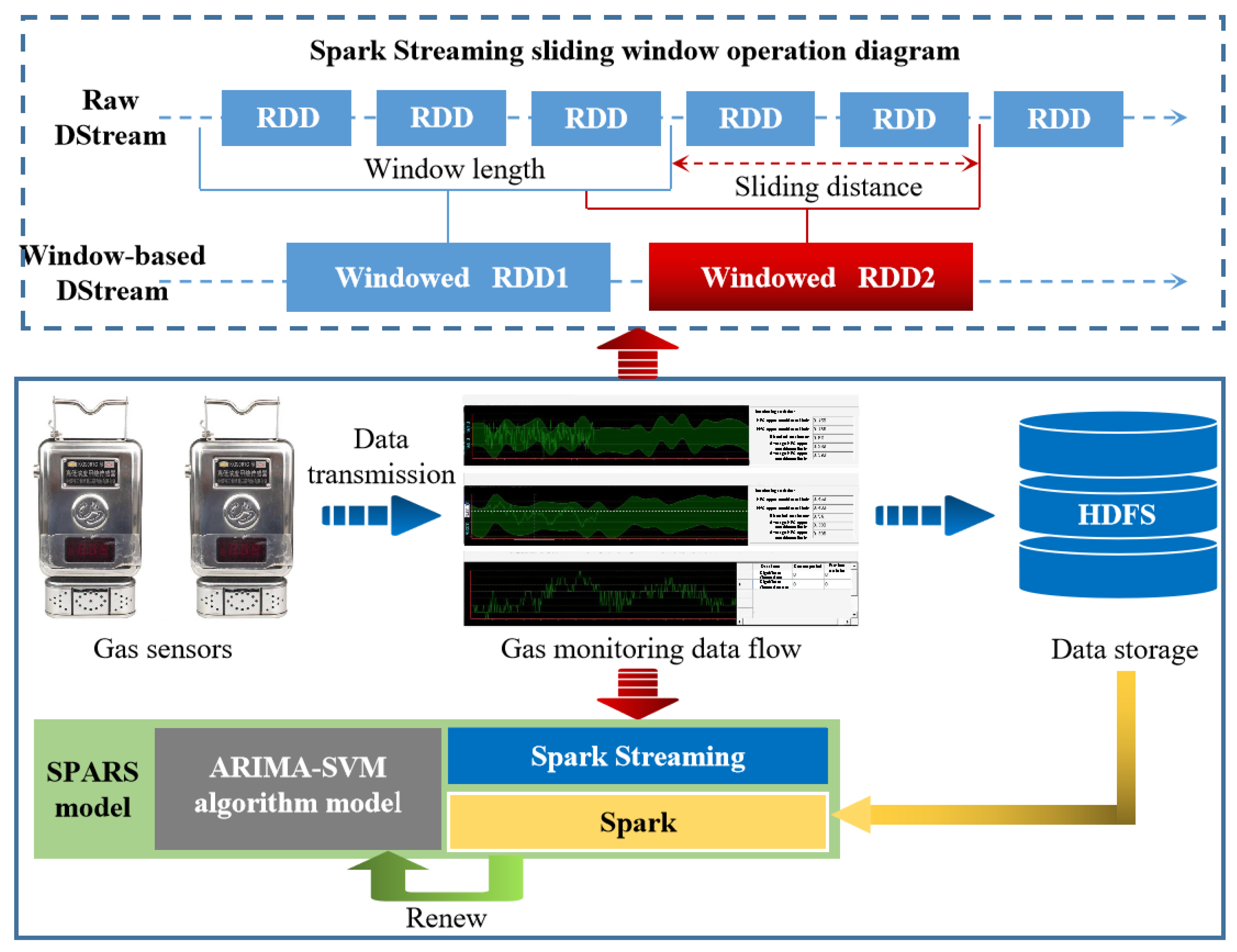
2.3. SPARS Model
3. Experiment
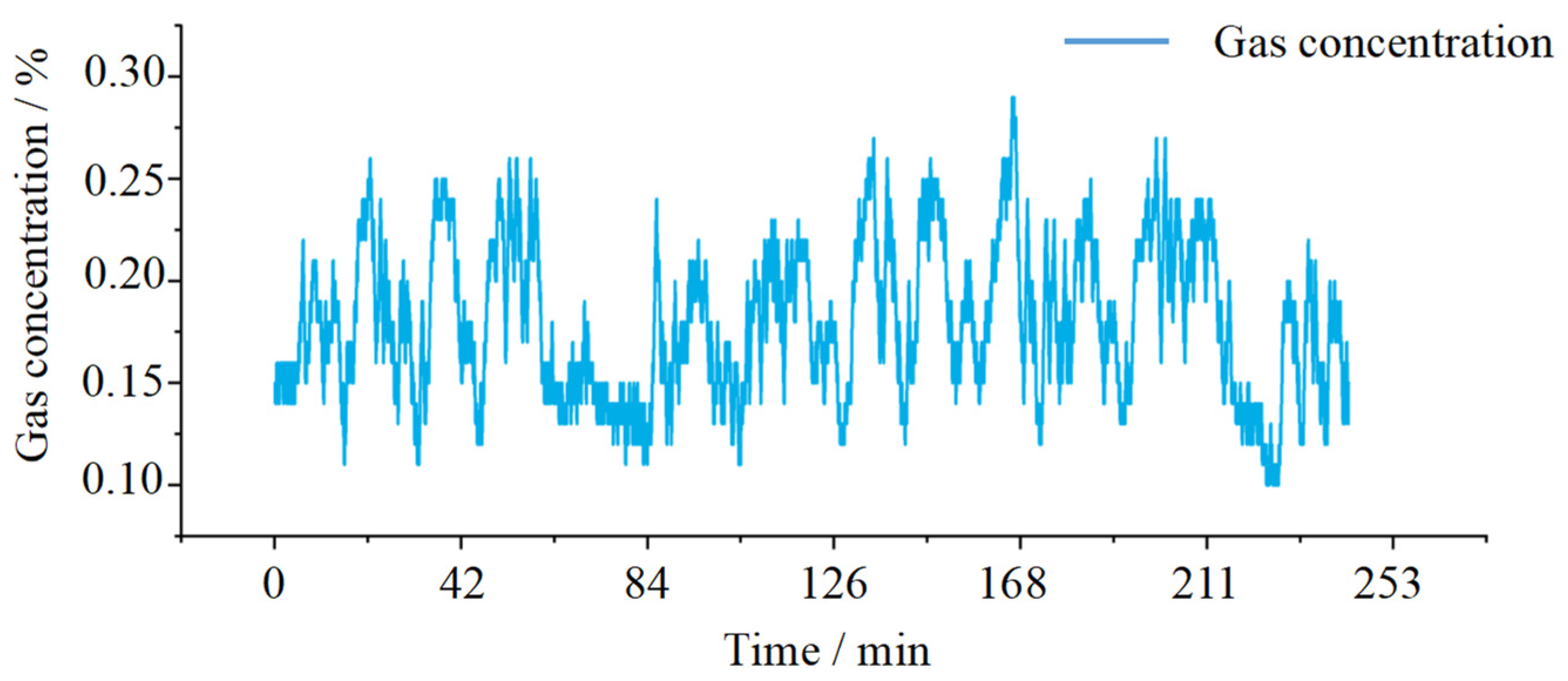
3.1. Data Sources
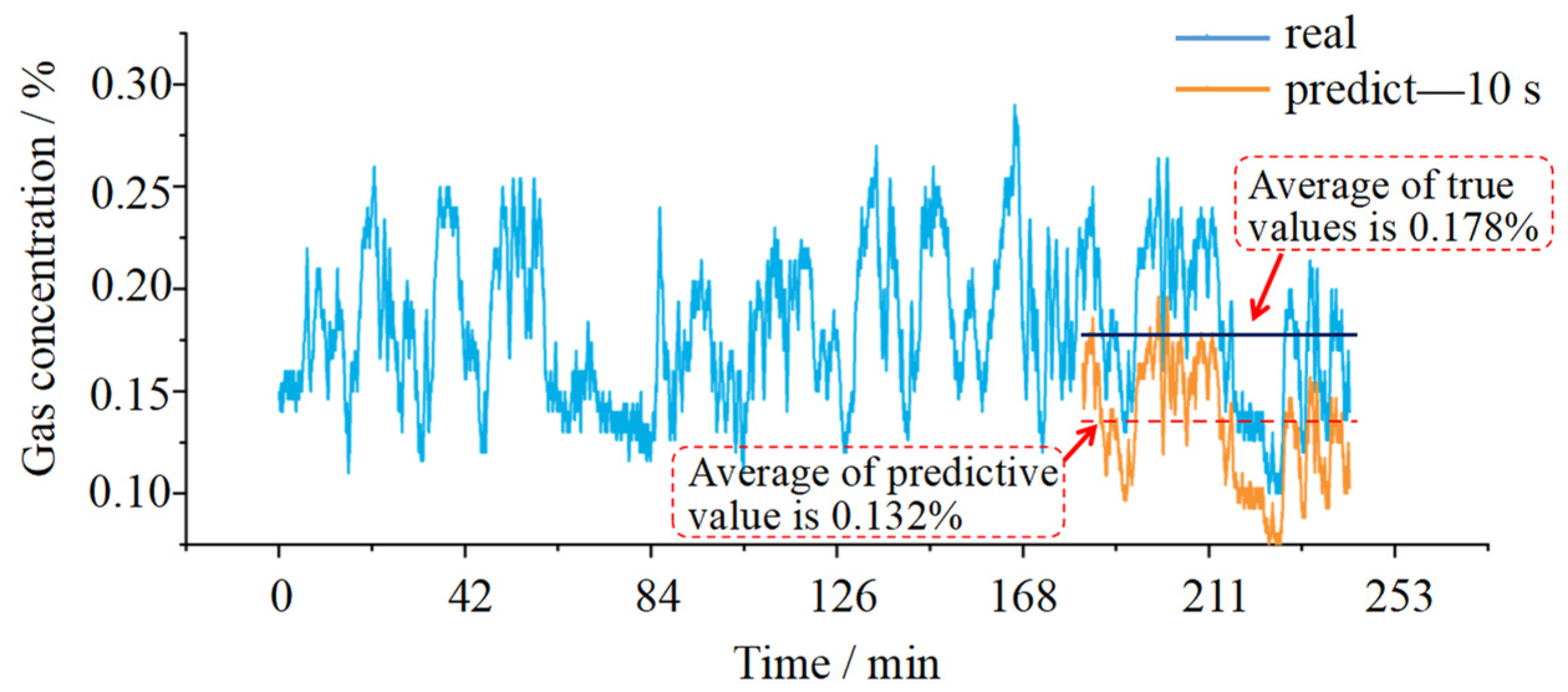
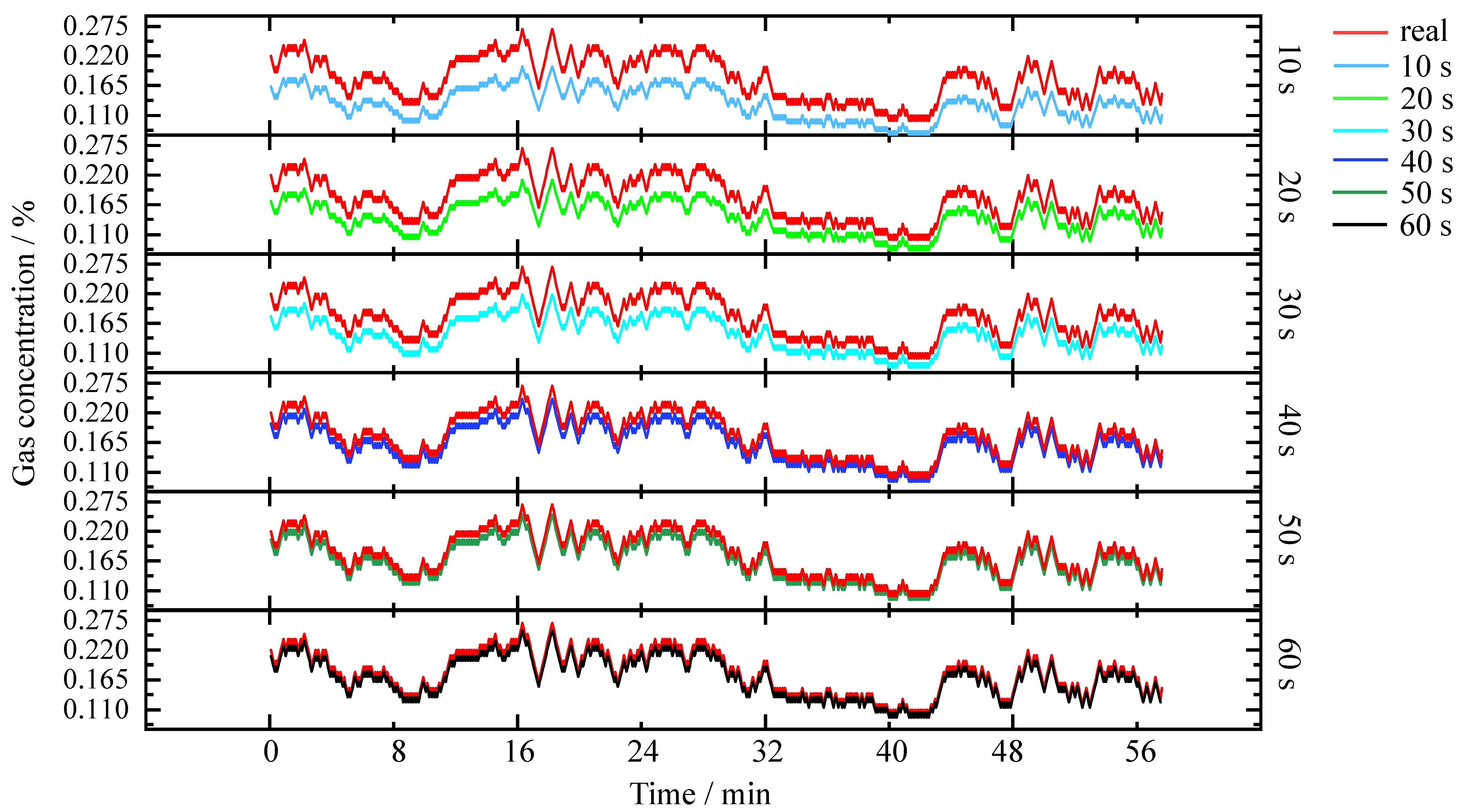
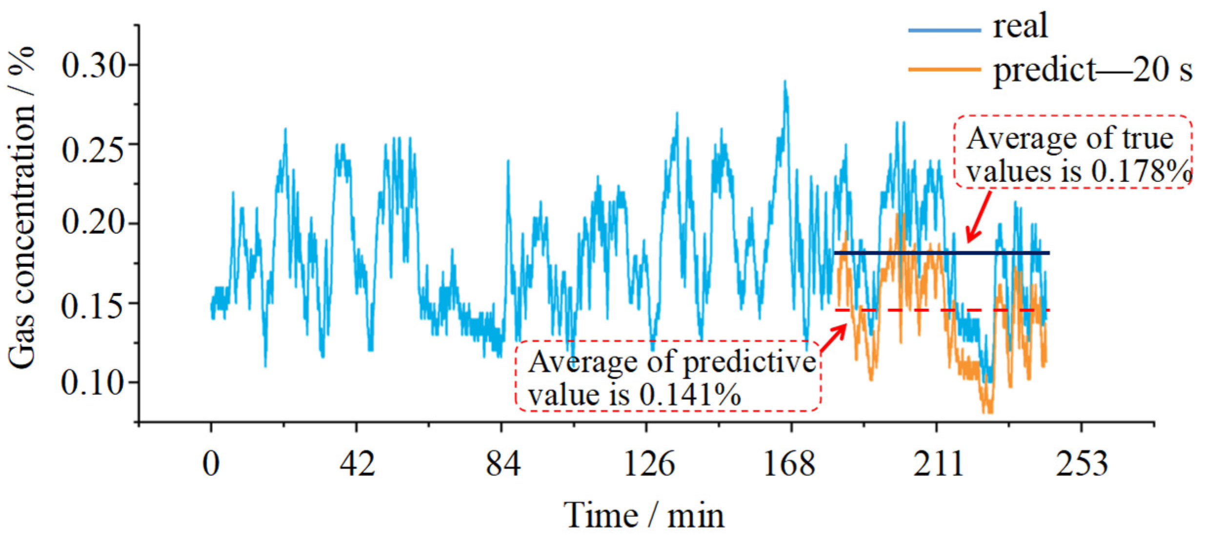
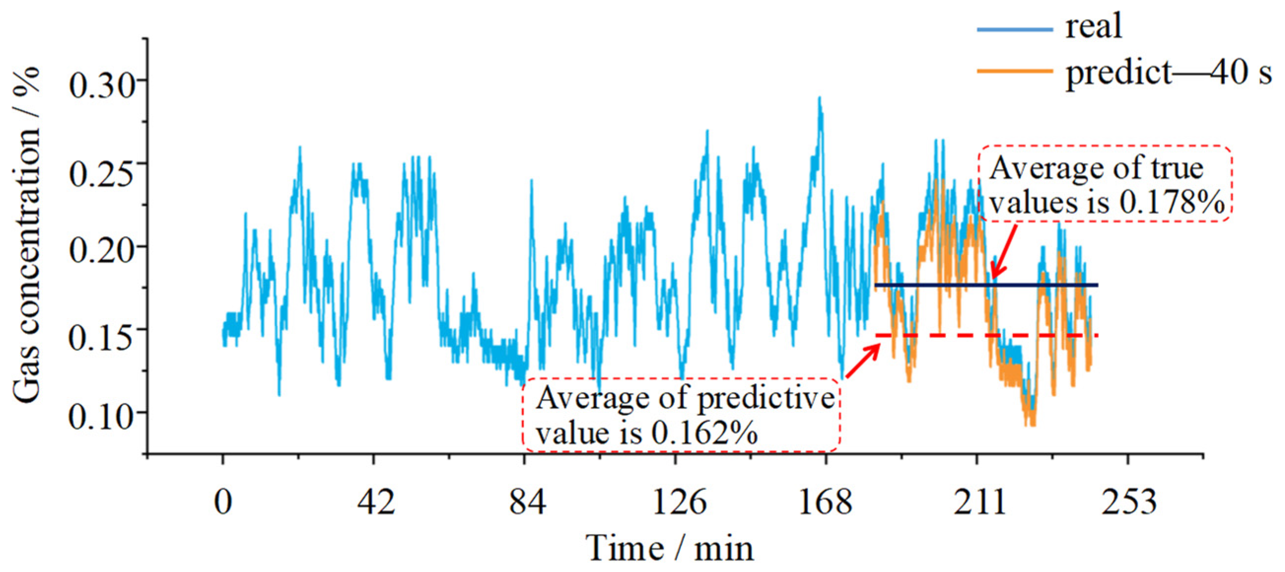
3.2. Prediction of the Gas Concentration by the SPARS Model
4. Discussion
5. Conclusions
Author Contributions
Funding
Acknowledgments
Conflicts of Interest
Abbreviations
| ARIMA | Autoregressive integrated moving average |
| SVM | Support vector machine |
| SPARS | Spark Streaming-autoregressive integrated moving average-support vector machine |
| CVS | Coal mine ventilation system |
| RDD | Resilient distributed dataset |
| HDFS | Hadoop distributed file system |
| TCP | Transmission control protocol |
| RMSE | Root mean square error |
References
- Cong, Y.; Zhao, X.; Tang, K.; Wang, G.; Hu, Y.; Jiao, Y. FA-LSTM: A Novel Toxic Gas Concentration Prediction Model in Pollutant Environment. IEEE Access 2022, 10, 1591–1602. [Google Scholar] [CrossRef]
- Zhang, Y.; Guo, H.; Lu, Z.; Zhan, L.; Hung, P.C. Distributed gas concentration prediction with intelligent edge devices in coal mine. Eng. Appl. Artif. Intell. 2020, 92, 103643. [Google Scholar] [CrossRef]
- Wang, X.Q.; Xu, N.K.; Meng, X.R.; Chang, H.Q. Prediction of Gas Concentration Based on LSTM-LightGBM Variable Weight Combination Model. Energies 2022, 15, 827. [Google Scholar] [CrossRef]
- Li, Y.; Yang, K.; Qin, R.; Yu, Y. Technical system and prospect of safe and efficient mining of coal and gas outburst coal seams. Coal Sci. Technol. 2020, 48, 167–173. [Google Scholar]
- Wang, G.; Yang, S.; Zhang, S.; Liu, X. Status and prospect of coal mine gas drainage and utilization technology in Xinjiang Coal Mining Area. Coal Sci. Technol. 2020, 48, 154–161. [Google Scholar]
- Zhang, J.; Ai, Z.; Guo, L.; Cui, X. Research of Synergy Warning System for Gas Outburst Based on Entropy-Weight Bayesian. Int. J. Comput. Intell. Syst. 2021, 14, 376–385. [Google Scholar] [CrossRef]
- Huang, Y.; Fan, J.; Yan, Z.; Li, S.; Wang, Y. Research on Early Warning for Gas Risks at a Working Face Based on Association Rule Mining. Energies 2021, 14, 6889. [Google Scholar] [CrossRef]
- Liang, R.; Chang, X.; Jia, P.; Xu, C. Mine Gas Concentration Forecasting Model Based on an Optimized BiGRU Network. ACS Omega 2020, 5, 28579–28586. [Google Scholar] [CrossRef]
- Zhang, X.Q.; Cheng, W.M.; Zhang, Q.; Yang, X.X.; Du, W.Z. Partition airflow varying features of chaos-theory-based coalmine ventilation system and related safety forecasting and forewarning system. Int. J. Min. Sci. Technol. 2017, 27, 269–275. [Google Scholar]
- Xu, Y.; Meng, R.; Zhao, X. Research on a Gas Concentration Prediction Algorithm Based on Stacking. Sensors 2021, 21, 1597. [Google Scholar] [CrossRef]
- Jia, P.; Liu, H.; Wang, S.; Wang, P. Research on a Mine Gas Concentration Forecasting Model Based on a GRU Network. IEEE Access 2020, 8, 38023–38031. [Google Scholar] [CrossRef]
- Wang, K.; Zhang, J.; Cai, B.; Yu, S. Emission factors of fugitive methane from underground coal mines in China: Estimation and uncertainty. Appl. Energy 2019, 250, 273–282. [Google Scholar] [CrossRef]
- Zhao, B.; Cao, J.; Sun, H.; Wen, G.; Dai, L.; Wang, B. Experimental investigations of stress-gas pressure evolution rules of coal and gas outburst: A case study in Dingji coal mine, China. Energy Sci. Eng. 2019, 8, 61–73. [Google Scholar] [CrossRef] [Green Version]
- Lu, Z.; Zhu, X.; Wang, H.; Li, Q. Mathematical modeling for intelligent prediction of gas accident number in Chinese coal mines in recent years. J. Intell. Fuzzy Syst. 2018, 35, 2649–2655. [Google Scholar] [CrossRef]
- Xiao, W.; Hu, J. SWEclat: A frequent itemset mining algorithm over streaming data using Spark Streaming. J. Supercomput. 2020, 76, 7619–7634. [Google Scholar] [CrossRef] [Green Version]
- Lee, Y.; Song, S. Distributed Indexing Methods for Moving Objects based on Spark Stream. Int. J. Contents 2015, 11, 69–72. [Google Scholar] [CrossRef] [Green Version]
- Wang, Y.; Guo, Y. Forecasting method of stock market volatility in time series data based on mixed model of ARIMA and XGBoost. China Commun. 2020, 17, 205–221. [Google Scholar] [CrossRef]
- Wang, J.; Sun, L.; Zhao, H.; Wang, Y. ARIMA-BP integrated intelligent algorithm for China’s consumer price index forecasting and its applications. J. Intell. Fuzzy Syst. 2016, 31, 2187–2193. [Google Scholar] [CrossRef]
- Svetunkov, I.; Boylan, J.E. State-space ARIMA for supply-chain forecasting. Int. J. Prod. Res. 2020, 58, 818–827. [Google Scholar] [CrossRef]
- Dawoud, I.; Kaçiranlar, S. An optimal k of kth MA-ARIMA models under a class of ARIMA model. Commun. Stat. Theory Methods 2017, 46, 5754–5765. [Google Scholar] [CrossRef]
- Xu, D.; Zhang, Q.; Ding, Y.; Zhang, D. Application of a hybrid ARIMA-LSTM model based on the SPEI for drought forecasting. Environ. Sci. Pollut. Res. 2022, 29, 4128–4144. [Google Scholar] [CrossRef] [PubMed]
- Bhandari, S.; Zhao, H.P.; Kim, H.; Khan, P.; Ullah, S. Packet Scheduling Using SVM Models in Wireless Communication Networks. J. Internet Technol. 2019, 20, 1505–1512. [Google Scholar]
- Jung, C.; Shen, Y.; Jiao, L. Learning to Rank with Ensemble Ranking SVM. Neural Process. Lett. 2015, 42, 703–714. [Google Scholar] [CrossRef]
- Zhang, T.; Song, S.; Li, S.; Ma, L.; Pan, S.; Han, L. Research on Gas Concentration Prediction Models Based on LSTM Multidimensional Time Series. Energies 2019, 12, 161. [Google Scholar] [CrossRef] [Green Version]
- Liang, Y.Q.; Guo, D.Y.; Huang, Z.F.; Jiang, X.H. Prediction model for coal-gas outburst using the genetic projection pursuit method. Int. J. Oil Gas Coal Technol. 2017, 16, 271–282. [Google Scholar] [CrossRef]
- Lim, S.; Yun, H. Forecasting Tanker Indices with ARIMA-SVM Hybrid Models. Korean J. Financ. Eng. 2018, 17, 79–98. [Google Scholar]
- Ordóñez, C.; Lasheras, F.S.; Roca-Pardiñas, J.; Juez, F.J.D.C. A hybrid ARIMA–SVM model for the study of the remaining useful life of aircraft engines. J. Comput. Appl. Math. 2019, 346, 184–191. [Google Scholar] [CrossRef]
- Chen, L.; Wang, E.; Feng, J.; Kong, X.; Li, X.; Zhang, Z. A dynamic gas emission prediction model at the heading face and its engineering application. J. Nat. Gas Sci. Eng. 2016, 30, 228–236. [Google Scholar] [CrossRef]
- Zhao, X.; Sun, H.; Cao, J.; Ning, X.; Liu, Y. Applications of online integrated system for coal and gas outburst prediction: A case study of Xinjing Mine in Shanxi, China. Energy Sci. Eng. 2020, 8, 1980–1996. [Google Scholar] [CrossRef]
- Tutak, M.; Brodny, J. Predicting Methane Concentration in Longwall Regions Using Artificial Neural Networks. Int. J. Environ. Res. Public Health 2019, 16, 1406. [Google Scholar] [CrossRef] [Green Version]
- Eckhoff, R.K. Testing of dust clouds for the electrostatic-spark ignition hazard in industry. Need for a modified approach? J. Loss Prev. Process Ind. 2021, 70, 104405. [Google Scholar] [CrossRef]
- Prats, D.B.; Portella, F.A.; Costa, C.H.A.; Berral, J.L. You Only Run Once: Spark Auto-Tuning From a Single Run. IEEE Trans. Netw. Serv. Manag. 2020, 17, 2039–2051. [Google Scholar] [CrossRef]
- Zheng, T.; Chen, G.; Wang, X.; Chen, C.; Wang, X.; Luo, S. Real-time intelligent big data processing: Technology, platform, and applications. Sci. China Inf. Sci. 2019, 62, 82101. [Google Scholar] [CrossRef] [Green Version]
- Guo, Z.; Zhang, Y.; Lv, J.; Liu, Y.; Liu, Y. An Online Learning Collaborative Method for Traffic Forecasting and Routing Optimization. IEEE Trans. Intell. Transp. Syst. 2021, 22, 6634–6645. [Google Scholar] [CrossRef]
- Ouyang, Q.; Lv, Y.B.; Ma, J.H.; Li, J. An LSTM-Based Method Considering History and Real-Time Data for Passenger Flow Prediction. Appl. Sci. 2020, 10, 3788. [Google Scholar] [CrossRef]
- Liew, J.; Göçmen, T.; Lio, W.H.; Larsen, G.C. Streaming dynamic mode decomposition for short-term forecasting in wind farms. Wind Energy 2022, 25, 719–734. [Google Scholar] [CrossRef]


| Time | Gas Concentration/% | Time | Gas Concentration/% |
|---|---|---|---|
| 8 July 2021 15:00:00 | 0.13 | 8 July 2021 15:00:40 | 0.14 |
| 8 July 2021 15:00:05 | 0.13 | 8 July 2021 15:00:45 | 0.12 |
| 8 July 2021 15:00:10 | 0.13 | 8 July 2021 15:00:50 | 0.13 |
| 8 July 2021 15:00:15 | 0.14 | 8 July 2021 15:00:55 | 0.14 |
| 8 July 2021 15:00:20 | 0.15 | 8 July 2021 15:01:00 | 0.15 |
| 8 July 2021 15:00:25 | 0.14 | 8 July 2021 15:01:05 | 0.14 |
| 8 July 2021 15:0030 | 0.14 | 8 July 2021 15:01:10 | 0.14 |
| 8 July 2021 15:00:35 | 0.13 | 8 July 2021 15:01:15 | 0.14 |
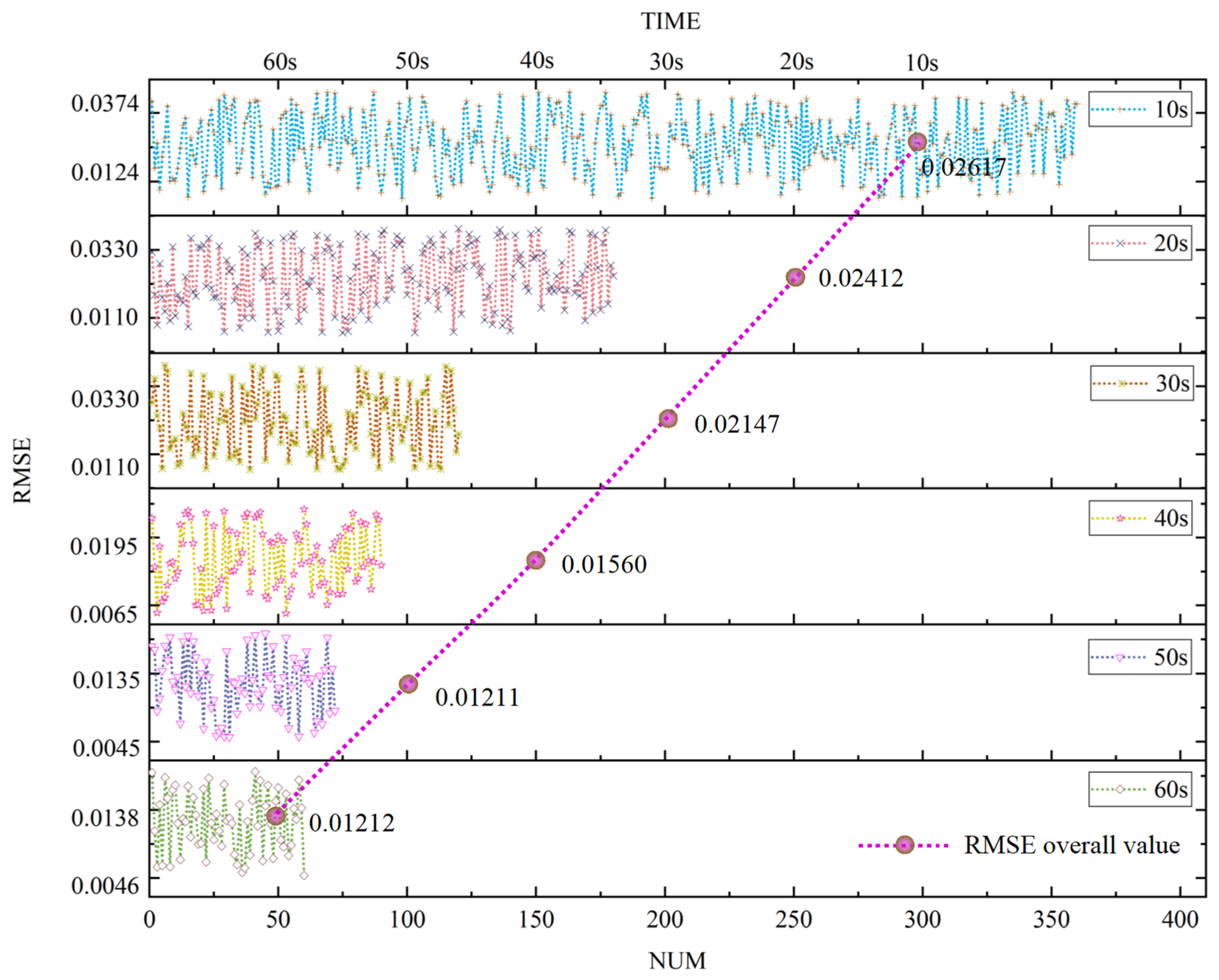
| Model Update Time | Number of Updates | Overall Value RMSE |
|---|---|---|
| 10 s | 360 | 0.02617 |
| 20 s | 180 | 0.02412 |
| 30 s | 120 | 0.02147 |
| 40 s | 90 | 0.0156 |
| 50 s | 72 | 0.01211 |
| 60 s | 60 | 0.01212 |
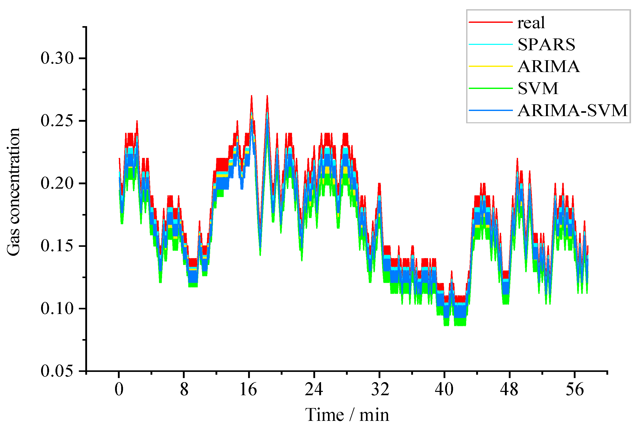
| Model | Maximum Error/% | Minimum Error/% | Average Error/% |
|---|---|---|---|
| SPARS | 0.0189 | 0.0070 | 0.0124 |
| ARIMA | 0.0270 | 0.0078 | 0.0162 |
| SVM | 0.0326 | 0.0127 | 0.0217 |
| ARIMA-SVM | 0.0208 | 0.0094 | 0.0145 |
Publisher’s Note: MDPI stays neutral with regard to jurisdictional claims in published maps and institutional affiliations. |
© 2022 by the authors. Licensee MDPI, Basel, Switzerland. This article is an open access article distributed under the terms and conditions of the Creative Commons Attribution (CC BY) license (https://creativecommons.org/licenses/by/4.0/).
Share and Cite
Huang, Y.; Fan, J.; Yan, Z.; Li, S.; Wang, Y. A Gas Concentration Prediction Method Driven by a Spark Streaming Framework. Energies 2022, 15, 5335. https://doi.org/10.3390/en15155335
Huang Y, Fan J, Yan Z, Li S, Wang Y. A Gas Concentration Prediction Method Driven by a Spark Streaming Framework. Energies. 2022; 15(15):5335. https://doi.org/10.3390/en15155335
Chicago/Turabian StyleHuang, Yuxin, Jingdao Fan, Zhenguo Yan, Shugang Li, and Yanping Wang. 2022. "A Gas Concentration Prediction Method Driven by a Spark Streaming Framework" Energies 15, no. 15: 5335. https://doi.org/10.3390/en15155335
APA StyleHuang, Y., Fan, J., Yan, Z., Li, S., & Wang, Y. (2022). A Gas Concentration Prediction Method Driven by a Spark Streaming Framework. Energies, 15(15), 5335. https://doi.org/10.3390/en15155335