Abstract
The scramjet of hypersonic vehicles faces severe high-temperature challenges, but the heat sink available for scramjet cooling is extremely finite. It is necessary to optimize its power and thermal management system (PTMS) with a finite heat sink of hydrocarbon fuel. This paper proposes a two-level optimization method for the PTMS of hypersonic vehicles at Mach 6. The PTMS is based on a supercritical carbon dioxide (SCO2) closed Brayton cycle, and its heat sink is airborne hydrocarbon fuel. System-level optimization aims to obtain the optimal system parameters for the PTMS. The minimum fuel weight penalty and the minimum heat sink consumption of fuel are the optimization objectives. The segmental (SEG) method is used to analyze the internal temperature distribution of fuel–SCO2 heat exchangers in the system-level optimal solution set. This ensures the selected optimal solutions meet the requirement of a pinch temperature difference greater than or equal to 10 °C. Further, the component-level optimization for the fuel–SCO2 heat exchanger is carried out based on the selected optimal solutions. The lightest weight of the heat exchanger and the minimum entropy production are the optimization objectives in this step. Finally, the optimal system parameters and the optimal key component parameters can be searched using this presented two-level optimization method.
1. Introduction
One of the key technologies of hypersonic flight is the cooling of the scramjet [1,2,3]. The combustion chamber of the scramjet is in a harsh thermal environment, which even the most advanced composite materials cannot withstand [4]. Traditional aircraft can use cooling air as a heat sink [5]. For hypersonic vehicles, airflow cannot be used as a heat sink due to the excessive temperature, so hydrocarbon fuel becomes the main heat sink [6]. Therefore, the hypersonic vehicle faces the tough problem of the finite heat sink. The design of the power and thermal management system (PTMS) should be paid more attention to.
The application of regenerative cooling technology in X-51A flight tests successfully verified the feasibility of scramjet cooling with endothermic hydrocarbon fuel [7]. It made full use of the chemical heat sink of fuel through the thermal cracking reaction in the cooling channels of the scramjet [8]. The PTMS based on fuel vapor turbine was proposed for the first time in the Hy-Tech program of the United States. In this system, the fuel pyrolysis vapor expands to drive the fuel pump [9]. Zhang et al. [10] evaluated the working capacity performance of the fuel vapor turbine and found that the fuel vapor turbine has enough power to drive a generator, in addition to a fuel pump. The closed Brayton cycle based on supercritical carbon dioxide (SCO2) utilizes SCO2 to exchange the high-temperature heat from the scramjet. This cycle avoids the direct heat exchange between the scramjet and fuel, which is easy to coke, and blocks the cooling channels when the incomplete pyrolysis reaction occurs [11,12,13]. Compared with hydrocarbon fuel, SCO2 is more reliable and stable [6]. It converts part of the high-temperature waste heat of the scramjet into electricity, and the fuel only needs to cool the residual heat. It can improve the cooling capacity of the fuel heat sink. Guo et al. [14] summarized the advantages and disadvantages of the above schemes and proposed a new PTMS based on a SCO2 cycle and a fuel vapor turbine. This PTMS met the cooling and high-power electricity demands at the same time for long-endurance hypersonic vehicles.
Many scholars conducted optimization research on the PTMS of hypersonic vehicles. Cheng et al. [6] optimized and compared the electric power performance between the simple recuperated and recompressing SCO2 cycles. They found that the former utilizes more cooling capacity of fuel. Miao et al. [12] compared the performance of three typical closed Brayton cycle layouts, namely simple, recuperated and SCO2 cycles. They proposed an improved scheme of the SCO2 cycle with lower cooling fuel consumption. Marchionni et al. [15] studied eight different SCO2 cycles and revealed that the complex SCO2 cycle configurations led to higher efficiency and costs. The existing studies on the PTMS of hypersonic vehicles mainly focused on system scheme design and thermodynamic characteristics optimization. So far, few studies considered the design of system-level and component-level optimization at the same time.
The total mass of the take-off period method is often used to evaluate the performance of airborne equipment [16,17]. It converts various losses caused by the analyzed system into the mass of fuel consumed to transport these masses and generate the required power [18]. Total fuel weight penalty can evaluate and compare different schemes of PTMSs.
Considering fuel weight penalty and power-to-weight Ratio (PWR), the closed Brayton cycle based on SCO2 for hypersonic vehicles usually adopts a printed circuit heat exchanger (PCHE) [13,19,20,21,22,23]. PCHE is a high-temperature heat exchanger that exchanges the heat from SCO2 to fuel. Because the physical properties of SCO2 and fuel vary greatly with temperature and pressure [12], it is necessary to adopt the segmental (SEG) method. It divides PCHE into several sub-heat exchangers, and then the detailed temperature of each sub-heat exchanger can be calculated [24]. The SEG method can be used to solve the question of the unreasonable pinch temperature difference and analyze the feasibility of heat transfer. Li et al. [24] proved that the maximum deviation between the heat exchange rate predicted by the SEG method and the experimental data was less than 5%. Entropy generation should also be considered while minimizing the weight of the heat exchanger [25]. Bejan stated that entropy generation should play a central role in heat transfer analysis [26]. Guo et al. proved that the heat transfer entropy generation is far larger than the frictional entropy generation by the SEG method [27].
For hypersonic vehicles with finite heat sink, a concerning goal is to optimize a PTMS to absorb as much heat and produce as much power as possible. In this paper, a two-level optimization method for the PTMS based on a SCO2 closed Brayton cycle is established by non-dominated sorting genetic algorithms (NSGA-II) [28,29]. Simulation models are validated using published experimental data. The effects of optimization variables on the PTMS are discussed in detail. Furthermore, the optimal parameters of the system and key components are determined, and further analysis is carried out to compare the optimization results.
2. Method
2.1. System Description
For the traditional regenerative cooling scheme for the scramjet, the hydrocarbon fuel is cracked in the cooling channels of the scramjet wall. This easily leads to coke and blocks cooling channels, which causes the scramjet to be scrapped after a long-endurance hypersonic flight. Therefore, the PTMS based on SCO2 closed Brayton cycle has been studied in recent years [6,12,13,14], as shown in Figure 1. It moves the easily coking process from the cooling channels of the scramjet wall to the fuel–SCO2 heat exchanger. Compared with the high cost of the scramjet, it is economical to replace the blocked heat exchanger. At the same time, the SCO2 scheme can convert part of scramjet waste heat into electric energy to meet the power demand of hypersonic vehicles. In the SCO2 cycle, PCHE is generally adopted for fuel–SCO2 heat exchangers because of its high heat transfer efficiency and because it is lightweight [13]. Considering the space limitations in the vehicle cabin, it is necessary to comprehensively balance between a thermal design and a geometric design of PCHE.
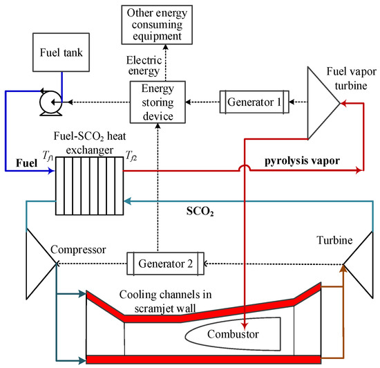
Figure 1.
Scheme of PTMS based on SCO2 closed Brayton cycle.
2.2. Two-Level Optimization Method
The two-level optimization method is presented to optimize the PTMS based on the SCO2 closed Brayton cycle with the finite heat sink of hydrocarbon fuel at 6 March. The inputs of the system-level optimization are fuel mass flow, heat production of the scramjet, and PWR of PCHE.
The multi-objective evolutionary algorithm, NSGA-II, is used to complete two-level optimization. It has been widely used in system optimization and heat exchanger design [29,30,31]. According to Ref. [29], the population size is set to 100, the number of generations is set to 100, the cross-over probability is set to 0.9, and the mutation probability is set to 0.1.
In the system-level optimization, the objective functions are to minimize the fuel weight penalty and heat sink consumption of fuel, which can be expressed by a vector:
where fs,1 (XS) and fs,2 (XS) represent min (Mtotal) and min (Qhs), respectively; XS represents the system-level optimization variable vector and can be expressed as:
where xs,1, xs,2 and xs,3 represent the compressor inlet pressure (PS,1, 7.4~11 MPa), heat exchanger efficiency (ηhx, 80~95%), and compressor pressure ratio (πC, 2~5), respectively.
The constraints in the system-level optimization are defined as follows:
where Tmax and Tc,0 represent the maximum temperature of the SCO2 cycle and outlet temperature of the cold side of PCHE, respectively.
After the system-level optimization, the SEG method is used to analyze the solution set of system-level optimization, which ensures the selected optimal solutions meet the pinch temperature difference (ΔTmin) greater than or equal to 10 °C. The component-level optimization for the fuel–SCO2 heat exchanger is carried out based on the above-selected solutions.
In component-level optimization, the objective functions can be expressed by a vector:
where fb,1 (Xb) and fb,2 (Xb) represent the lightest weight and the minimum entropy production (Sg) of PCHE, respectively; Xb represents the component-level optimization variable vector and can be expressed as:
where xb,1, xb,2 and xb,3 represent the channel width (wc, 1~2 mm), core width (W, 0~1 m) and core height (H, 0~1 m), respectively.
The constraints in the component-level optimization are defined as follows:
where Ploss and L represent pressure loss in PCHE and channel length, respectively.
It takes the lightest weight of PCHE and the minimum.
The two-level optimization process is shown in Figure 2.
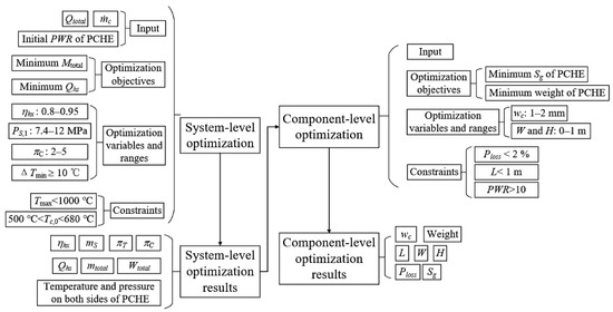
Figure 2.
Two-level optimization process.
The basic parameters of optimization are shown in Table 1.

Table 1.
Basic parameters of optimization.
3. Simulation Model and Its Verification
3.1. Simulation Model
(1) Cooling channel model in the scramjet wall
Referring to X-51A, the fuel mass flow rate is 0.5 kg/s at Mach 6 [7]. According to the classic Lander–Nixon diagram, the demand for fuel heat sink capacity for scramjet cooling is about 1.8~2.7 MJ/kg at Mach 6 [32]. For safety reasons, the maximum value of 2.7 MJ/kg is selected in this paper. Thus, the heat production of the scramjet is 1350 kW. All the scramjet heat is assumed to be taken away by SCO2 in the cooling channels.
The relative pressure loss coefficient in cooling channels is defined as follows:
where PS,2 and PS,3 are the inlet and outlet pressures of cooling channels, respectively, MPa; ξcc is the relative pressure loss coefficient in cooling channels and is set to 2% according to Ref. [12].
(2) Turbomachinery model
This type of single-stage radial turbomachinery is adopted in this paper because the power output is less than 300 kW [33,34,35]. For the compressor and turbine, isentropic efficiencies are respectively defined as:
where ηC and ηT are the isentropic efficiencies of compressor and turbine, respectively, %; hS,1, hS,2 and hS,2s are the inlet specific enthalpy, the outlet specific enthalpy, and the ideal outlet specific enthalpy of the compressor, respectively, kJ/kg; hS,3, hS,4 and hS,4s are the inlet specific enthalpy, the outlet specific enthalpy and the ideal outlet specific enthalpy of the turbine, respectively, kJ/kg.
Balje’s chart summarized the dimensionless parameters of the total efficiency for the turbine and compressor. The specific speed and specific diameter are calculated as [36]:
where Ns is the specific speed; Ds is the specific diameter; D is the diameter, m; N is shaft speed, rad/min; V is the volume flow rate, m3/s; Had is the adiabatic enthalpy increase, kJ.
For the SCO2 cycle, the following formulas are adopted [37]:
The weight of turbomachinery is calculated as [38]:
where m is the weight of the turbomachinery, kg; k0 is the weight coefficient, and k0 = 180 [38,39].
(3) Heat exchanger model
In the SCO2 cycle, the PCHE is selected because of its high-heat transfer efficiency and low weight and volume [13]. The physical properties of SCO2 dramatically change near its critical point. To obtain higher accuracy, the SEG method is used to complete the design of PCHE. The PCHE adopts a semicircular straight channel because of its low pressure loss coefficient. The basic configuration of PCHE is shown in Figure 3 [24].
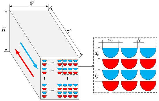
Figure 3.
PCHE configuration and basic parameters.
In this paper, Incoloy 907 is selected as the material of PCHE, and its maximum allowable temperature is about 1000 °C [40]. The porosity of PCHE is ϕ = 75.8%. The dimensions of the channels are dc/wc = 0.5, tP/wc = 0.51, and tf/wc = 0.015.
The heat transfer of PCHE is assumed to be one-dimensional along its flow direction and ignores its heat transfer to the environment [24]. Then, the PCHE is divided into n sub-heat exchangers with the same heat exchange capability, as shown in Figure 4. So, Qi = Qtotal/n and n = 20 in this paper [27]. Th,i−1 and Tc,i represent hot side and cold side inlet temperatures of the ith sub-heat exchanger, separately. Ph,i−1 and Pc,i represent hot side and cold side inlet pressures of the ith sub-heat exchanger, separately. The size, weight, and other parameters of PCHE can be obtained by the following formulas.
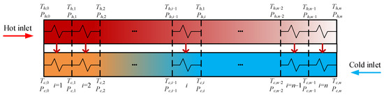
Figure 4.
Schematic diagram of SEG method.
For the sub-heat exchanger i, the local energy balance is defined as Equation (15):
where Qi is the heat transfer of each sub-heat exchanger, kW; m is the mass flow rate, kg/s; h is the specific enthalpy, kJ/kg; Subscripts h and c represent the hot side and cold side of the heat exchanger, respectively.
The local heat transfer equation can be given as Equation (16):
where As,h represents the heat exchange area of the hot side, m2; U represents the total convective heat transfer coefficient; and kW/(m2·K), and is calculated with Equation (17):
where tw represents wall thickness, mm; kw represents the thermal conductivity of metal wall, kW/(m·K); As,w represents the heat exchange area of metal wall, m2; α represents the heat transfer coefficient; and kW/(m2·K); ηt represents the overall surface efficiency defined in Equation (18):
where wc represents the channel width, m; ηf represents the fin efficiency of the semicircular channel, and is defined in Equation (19):
where m and t* are dimensionless numbers and normalized fin thickness, separately.
m and t* are calculated with Equations (20) and (21), separately:
where λ represents the thermal conductivity of the fluid, kW/(m·K); Nu is the Nusselt number.
The following formulas are used to calculate laminar and turbulent [24], separately.
where f is fanning friction factor; Re and Pr are the Reynolds number and Prandtl number, separately.
The hydraulic diameter is calculated with Equation (24):
The pressure drop is calculated with Equation (25):
where Li is the length of each sub-heat exchanger; G is the mass flow flux, kg/(m2·s); ρi is the density of the fluid, kg/m3.
The weight, efficiency, PWR, and pressure loss of PCHE are calculated with Equations (26)–(29), separately:
where ρw is the density of metal wall, kg/m3; N is the number of channels; L is channel length, m; ϕ is porosity; ṁ is the mass flow rate of the fluid, kg/s; Ploss is hot side pressure loss of PCHE, %; ΔP is the hot side pressure drop of PCHE, MPa; Ph is hot side inlet pressure of PCHE, MPa.
The initial PWR is estimated to be 10 when the channel width is 1~2 mm. When the fluid inlet parameters on both sides of PCHE are determined, the scheme process of the SEG method is shown in Table 2 [24]:
Table 2.
Scheme process of the SEG method.
(4) Fuel vapor turbine model
The specific power generation of the fuel vapor turbine can be calculated with Equation (30) [11]:
where wf,m is the specific power generation of fuel vapor turbine, kJ/kg; p is the average specific heat of fuel, kJ/(kg·K); πfT is pressure drop ratio of fuel vapor turbine; k is the specific heat ratio of fuel.
Then, the total power generation of the fuel vapor turbine, Wf, can be calculated.
(5) Fuel weight penalty calculation
In this paper, the total mass of the take-off period method is employed [16,17,18]. The mass and power consumption of the PTMS can be converted into fuel consumption to evaluate their impact on the performance of the vehicle. Ignoring the weight of the fixed pipeline and power consumption of the fuel pump, the total fuel weight penalty of the PTMS is calculated with Equations (31) and (32) [16]:
where Mtotal is the total fuel weight penalty of the PTMS, kg; Mhx, MC, MT, and MfT are the fuel weight penalty values of PCHE, compressor, turbine in the SCO2 cycle, and fuel vapor turbine, kg; m indicates weight, kg; Ce is the specific fuel consumption, kg/(N·s); τ0 is the endurance time, s; g is gravitational acceleration, m/s2; K is the lift–drag ratio of the aircraft, and is 2.95 at 6 Mach [42]; TSFC is the thrust-specific fuel consumption, s−1, and is 0.001 at 6 Mach [43].
(6) System scheme design
The system scheme design process is shown in Figure 5. Firstly, the initial parameters, Tc,n, ηC, ηS,T, ηP, ηhx, ξhx, ξcc, P1, πC, are given. Based on the criterion of ΔTmin ≥ 10 K, the compressor inlet temperature, TS,1, is assumed. Then, the parameters of the SCO2 cycle and fuel can be obtained under the constraint of Tc,0 < TS,4. Finally, the optimized parameters are obtained.
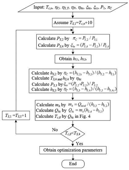
Figure 5.
System scheme design process.
3.2. Model Validation
For the cooling channel model, the heat exchange capacity is assumed to be 1350 kW according to the Lander–Nixon diagram [32]. For the fuel vapor turbine model, its parameters to calculate power generation refer to the experimental results in Ref. [11].
The turbomachinery model is verified using published experimental data. The comparison between simulation and experimental results of impeller diameter is shown in Table 3. The experimental data for compressor and turbine are taken from Refs. [44,45], respectively. The differences are 2.7% and 4.7% respectively, and both are less than 5%.
Table 3.
Verification of turbomachinery model.
The heat exchanger model is verified using published experimental data [46]. Experimental parameters of PCHE are shown in Table 4. The comparisons of ηhx at different Th,0 between experiment and simulation results are shown in Table 5. Their differences are less than 3%.
Table 4.
Experimental parameters of PCHE.
Table 5.
Verification of heat exchanger model.
4. Results and Analysis
4.1. System-Level Optimization
It is assumed that the heat production of the scramjet is 1350 kW at Mach 6. The objective of the system-level optimization is to minimize the consumption of fuel heat sink and the fuel weight penalty. The preliminary optimization solution set is shown in Figure 6, in which the abscissa and the ordinate represent the consumption of the fuel heat sink and the fuel weight penalty, separately. In Figure 6, a point is highlighted with a triangle as an example point. It can be seen that Qhs is less than the heat production of the scramjet (1350 kW). This is because SCO2 converts part of the high-temperature waste heat of the scramjet into electricity, and the fuel only needs to cool the residual heat.
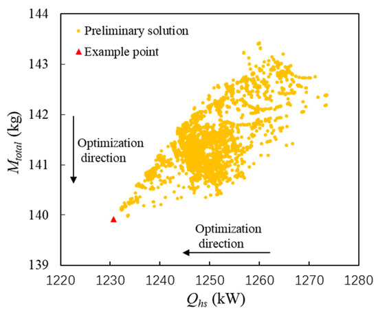
Figure 6.
Preliminary optimization solution set and the example point of PTMS.
However, the pinch point may be located inside the fuel–SCO2 heat exchanger, because the physical properties of SCO2 and fuel vary greatly with the change of temperature and pressure [12,24,47]. The internal temperature distribution of PCHEs in the solution set will be further analyzed using the SEG method to ensure the selected solutions meet ΔTmin ≥ 10 °C.
Taking the example point in Figure 6 as an example, the inlet pressure, temperature, and mass flow rate of the PCHE hot side are 7.5 Mpa, 773 °C, and 1.54 kg/s, respectively. The corresponding values on the cold side are 4 MPa, 50 °C, and 0.5 kg/s, respectively. The amount of heat exchange is 1231 kW. Based on these parameters, the variation curve of the water equivalent (cp × ṁ) with temperature is shown in Figure 7a. The square point represents the point with the lowest temperature difference. It can be seen that the temperature difference between SCO2 and fuel is the lowest near 377 °C. Figure 7b shows the temperature change curve in the ith (i = 1~20) sub-heat exchanger with the SEG method. The arrow indicates the solution direction. The fluid temperature difference on both sides gradually becomes smaller, and it is less than 10 K after the 10th sub-heat exchanger. In the 11th sub-heat exchanger, the fluid temperatures on both sides are crossed, but this heat reversal is impossible. This illustrates that the heat exchange process cannot occur under the given conditions. Therefore, these unfeasible solutions should be removed from the preliminary optimization set.
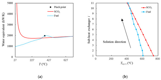
Figure 7.
Heat exchange process of example point. (a) Variation curve of water equivalent with the temperature. (b) Temperature variation curve of sub-heat exchanger.
In Figure 8, the selected solutions are marked in black squares to distinguish them from the preliminary solutions in the yellow circle. Circular points represent the infeasible solution, and square points represent the feasible solution.
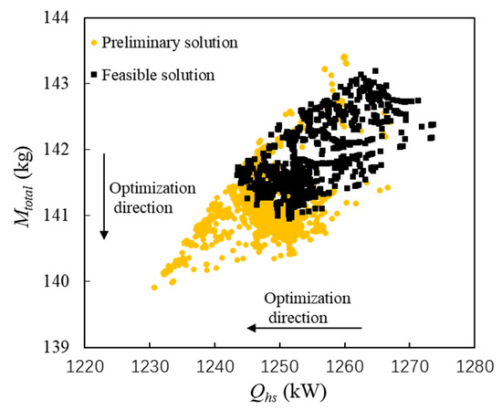
Figure 8.
System-level optimization results after feasible selection with SEG method.
Figure 9 shows the influence of hot side temperature and efficiency on the heat sink consumption of fuel. To ensure the heat exchange process occurring in PCHE, namely ΔTmin ≥ 10 °C, the hot side inlet temperature of the first sub-heat exchanger (Th,0) cannot be too low. The green line in Figure 9a shows the boundary of Th,0, which is 770~800 °C. Similarly, the heat exchanger efficiency cannot be too high. The green line in Figure 9b shows the boundary of ηhx, which is 90~91%. Th,0 and ηhx are consistent with the experimental results [47].
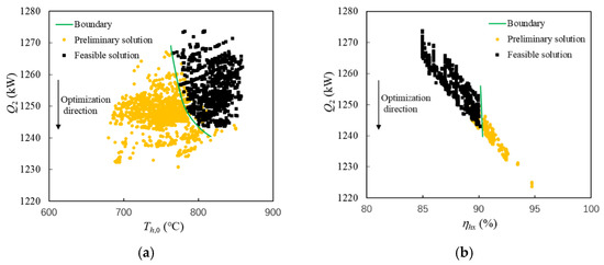
Figure 9.
Relationship of Th,0, ηhx and Qhs in feasible solutions. (a) Hot side inlet temperature boundary (b) Efficiency boundary.
Pareto points (A~F) and the Pareto front of the above feasible solutions are shown in Figure 10. The minimum consumption of fuel heat sink corresponds to the abscissa, and the minimum fuel weight penalty corresponds to the ordinate. The square points in black represent the non-dominated solutions, the triangle points in red represent the dominated solutions, and the solid line is the Pareto optimal front. A point is highlighted with a yellow circle as a reference system. The system parameters of Pareto points are shown in Table 6.
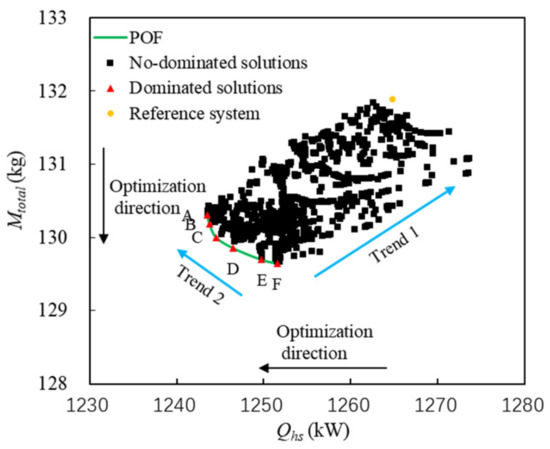
Figure 10.
System-level optimization results.
Table 6.
System parameters of Pareto points.
- (1)
- Fuel weight penalty mainly depends on the weight of PCHE, compressor, and turbines. The weight of PCHE is much greater than that of other components. The initial PWR of PCHE is fixed at 10, so the weight of PCHE depends on the heat exchange capability. Therefore, in the direction shown by Trend 1 in Figure 10, the greater Qhs, the greater Mtotal.
- (2)
- For Pareto points of A~F in the direction shown by Trend 2, there is a conclusion opposite to Trend 1. When Qhs is the maximum value of 1251.6 kw, Mtotal is the minimum of 129.6 kg. When Qhs is the minimum value of 1243.6 kw, Mtotal is the maximum of 130.3 kg. This is because the weight of turbomachinery decreases significantly with the increase in Qhs. Qhs and Mtotal become two competitive optimization variables. When Qhs decreases, Mtotal increases accordingly, and vice versa. The Pareto points are located in the regions close to the coordinate axes.
- (3)
- The slope of the Pareto front changes significantly near point C (1244.6 kW, 130.0 kg). When Qhs is less than 1244.6 kW, Mtotal increases significantly with the decrease in Qhs. When Qhs is greater than 1244.6 kW, the change rate of Mtotal decreases with the increase in Qhs. Thus, point C can be considered as a compromise between Mtotal and Qhs.
The relationships between optimization variables and objectives are shown in Figure 11.
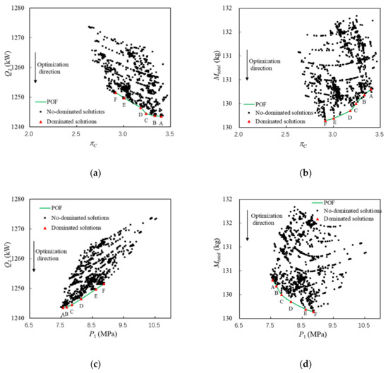
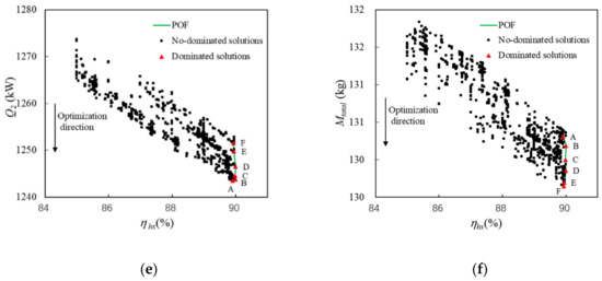
Figure 11.
Relationships between optimization variables and optimization objectives. (a) πC and Qhs (b) πC and Mtotal. (c) P1 and Qhs (d) P1 and Mtotal. (e) ηhx and Qhs (f) ηhx and Mtotal.
- (1)
- On the whole, increasing πC or reducing P1 not only reduces Qhs, but also increases Mtotal. When ηhx is less than 91%, increasing ηhx can reduce Qhs and Mtotal at the same time. Pareto points of A~F have approximately the same ηhx.
- (2)
- Tc,n and ṁc are constants, so Qhs depends on Ph, Th,0, ṁh, and ηhx from Section 3. Among the above factors, only Ph and Th,0 change significantly, as shown in Table 6. However, Qhs decreases with the increase in Th and the decrease in Ph, which indicates that Ph is the main influencing factor of Qhs.
- (3)
- For Pareto points, Mtotal mainly depends on the weight of turbomachinery. Increasing πC or decreasing P1 leads to a decrease in Had, which in turn leads to an increase in the weight of the turbomachinery from Equations (10)–(14).
4.2. Component-Level Optimization
The component-level optimization is carried out based on the optimal parameters of point C. The lightest weight of PCHE and the minimum entropy production are the optimization objectives. The optimization results are shown in Figure 12. C1~C8 are Pareto points, and the curve is the Pareto front. Entropy production includes heat transfer entropy production (SgT) and pressure entropy production (SgP), which affect the efficiency and pressure loss of PCHE, separately. The relationship curve between SgT and SgP is shown in Figure 13. The detailed parameters of C1~C8 are shown in Table 7.
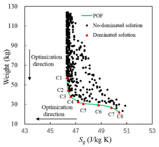
Figure 12.
Component-level optimization results.
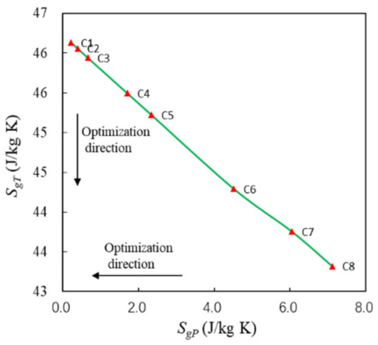
Figure 13.
The relationship between SgP and SgT.
Table 7.
Parameters of C1~C8.
As can be seen from Figure 12, the weight of PCHE decreases from 57.2 kg to 22.2 kg, and Sg increases from 46.3 J/kg·K to 50.4 J/kg·K. Pareto optimal solutions compete with each other, which proves that the weight is reduced at the cost of increasing irreversibility in PCHE. C1~C3 are almost perpendicular to the ordinate, reflecting significant weight reduction. C5~C8 are almost perpendicular to the abscissa, reflecting that the significant increase in Sg. L of C5 is more than 1m, so C3 and C4 can be considered as better choices.
As can be seen from Figure 13, SgT decreases only slightly, so the efficiency of PCHE is almost constant and stable at 90%. With the increase in SgP, Ploss increases from 0.14% to 0.49%. The pressure losses of C3 andC4 are less than 1% and meet the design requirements [20].
C4 is selected, considering its lighter weight and smaller volume. Thus, the optimal efficiency (89.84%) and PWR (38.0) of PCHE are obtained, and the optimal total fuel weight penalty can be calculated as 48.6 kg. According to Equations (2)–(14), the weight and dimensional design of the compressor, turbine in the SCO2 cycle and fuel vapor turbine are calculated as shown in Table 8.
Table 8.
Weight and dimensional design of turbomachinery.
The fuel weight penalty of each component is shown in Figure 14. The compressor and turbine are compact components, and the maximum weight is no more than 10 kg, which is consistent with Ref. [34]. The total fuel weight penalty mainly depends on the weight of PCHE, which is greater than the sum of other components.
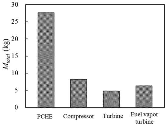
Figure 14.
The fuel weight penalty of each component.
To compare the optimization effect, the reference system and optimization system of C and C4 are used to compare the parameters before and after the two-level optimization. The comparison of optimization results is shown in Figure 15.
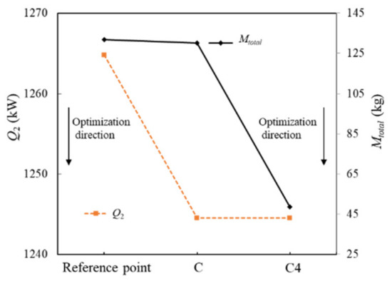
Figure 15.
Comparison of optimization results.
It can be seen from Figure 15 that the system-level optimization mainly reduces the heat sink consumption of fuel, and the component-level optimization mainly reduces the fuel weight penalty. The system-level optimization can reduce the heat sink consumption of fuel by 20.2 kW and the fuel weight penalty by 1.9 kg. Based on the optimal solution in the system-level optimization, the weight of PCHE can be reduced from 124.5 kg to 30.9 kg in the component-level optimization. Accordingly, the total fuel weight penalty can be further reduced by 83.3 kg.
5. Conclusions
In this study, a two-level optimization method for the PTMS is proposed by NSGA-Ⅱ for hypersonic vehicles at Mach 6. The PTMS is based on a SCO2 closed Brayton cycle with finite chemical heat sink of hydrocarbon fuel. The following conclusions can be obtained:
- (1)
- The system-level optimization can obtain the preliminary solution set. To ensure the feasibility of heat exchanger design, the SEG method is employed to analyze the detailed heat transfer process in PCHE. The minimum temperature difference of PCHE is limited to 10 °C, and the unfeasible solutions are removed. The minimum Th,0 is 770~800 °C, and the maximum ηhx is 90% in feasible solutions.
- (2)
- The turbomachinery adopts compact components, and their optimal design parameters are given. The results of the component-level optimization show that the weight of PCHE is greater than the sum of other components, and the total fuel weight penalty mainly depends on the weight of PCHE.
- (3)
- The proposed two-level optimization method gives the optimal system parameters and the optimal size of key components. It can reduce the heat sink consumption of fuel by 20.2 kW and the fuel weight penalty by 85.2 kg compared to the reference system.
Author Contributions
Conceptualization, X.Y.; Data curation, L.P. and X.Y.; Formal analysis, L.G. and J.Z.; Methodology, L.P., J.Z. and X.Y.; Resources, L.P.; Supervision, L.P.; Validation, J.Z.; Visualization, L.G.; Writing—original draft, L.G.; Writing—review & editing, L.G., L.P., J.Z. and X.Y. All authors have read and agreed to the published version of the manuscript.
Funding
This research received no external funding.
Institutional Review Board Statement
Not applicable.
Informed Consent Statement
Not applicable.
Data Availability Statement
All data is available in this paper.
Conflicts of Interest
No potential conflict of interest was reported by the authors.
Abbreviations
| Symbol | Denotation |
| πC | Compressor pressure ratio |
| πfT | Pressure drop ratio of fuel vapor turbine |
| πT | Pressure drop ratio of turbine in SCO2 cycle |
| C | The efficiency of compressor, % |
| G | The efficiency of the generator, % |
| P | The efficiency of the fuel pump, % |
| S,T | The efficiency of turbine in SCO2 cycle, % |
| ηhx | Heat exchanger efficiency, % |
| ηfT | The efficiency of fuel vapor turbine, % |
| cc | Relative pressure loss coefficient in cooling channels, % |
| hx | Relative pressure loss coefficient of PCHE, % |
| hx,s | Relative pressure loss coefficient of PCHE in system-level optimization, % |
| ṁc | Fuel mass flow rate, kg/s |
| ṁh | SCO2 mass flow rate, kg/s |
| As | Cross area, m2 |
| Ce | The specific fuel consumption, kg/(N·s) |
| core | Heat exchanger core |
| dc | Channel depth, mm |
| dh | Hydraulic diameter, mm |
| G | Mass flow flux, kg/(m2·s) |
| hS,2 | Compressor outlet-specific enthalpy, kJ/kg |
| hS,3 | Turbine inlet-specific enthalpy, kJ/kg |
| hS,2s | Ideal outlet-specific enthalpy of the compressor, kJ/kg |
| hS,24 | Ideal outlet-specific enthalpy of the turbine, kJ/kg |
| H | Core height of PCHE, m |
| K | Lift–drag ratio |
| L | The channel length of PCHE, m |
| Li | The channel length of each subheat exchanger, m |
| M | Weight of PCHE, kg |
| Mtotal | Total fuel weight penalty, kg |
| Ns | Specific speed |
| P1 | Compressor inlet pressure |
| POF | Pareto front |
| Ph | Hot side inlet pressure of PCHE, MPa |
| Ploss | Pressure loss of PCHE, % |
| Pp,in | Inlet pressure of the fuel pump, MPa |
| Pp,out | Outlet pressure of the fuel pump, MPa |
| PS,1 | Compressor inlet pressure, MPa |
| PS,2 | Compressor outlet pressure, MPa |
| PS,3 | Cooling channel outlet pressure, MPa |
| PS,4 | Turbine outlet pressure, MPa |
| PWR | Power-to-Weight Ratio of PCHE |
| Qhs | Heat sink consumption of fuel, kW |
| Qtotal | Engine heat production, kW |
| Sg | Total entropy production, J/kg·K |
| SgP | Pressure entropy production, J/kg·K |
| SgT | Heat transfer entropy production, J/kg·K |
| tf | Fin thickness, mm |
| tp | Plate width, mm |
| tw | Wall thickness, mm; |
| Tc,0 | The outlet temperature of the cold side of PCHE, °C |
| Tc,n | The inlet temperature of the cold side of PCHE, °C |
| Th,0 | The hot side inlet temperature of the first sub-heat exchanger, °C |
| Tmax | The maximum temperature of the SCO2 cycle, °C |
| TS,1 | Compressor inlet temperature |
| TS,4 | Turbine outlet temperature |
| TSFC | Thrust-specific fuel consumption, s-1 |
| wc | Channel width, mm |
| W | Core width of PCHE, m |
| ΔTmin | Pinch temperature difference |
References
- Office of Space Systems Development. NASA Headquarters, Access to Space Study: Summary Report; NASA-TM-109693, 1994-01.1994; NASA: Washington, DC, USA, 1994. [Google Scholar]
- Wu, X.; Yang, J.; Zhang, H.; Shen, C. System design and analysis of hydrocarbon scramjet with regeneration cooling and expansion cycle. J. Therm. Sci. 2015, 24, 350–355. [Google Scholar] [CrossRef]
- Dong, Y.; Wang, E.; You, Y.; Yin, C.; Wu, Z. Thermal protection system and thermal management for combined-cycle engine: Review and prospects. Energies 2019, 12, 240. [Google Scholar] [CrossRef] [Green Version]
- Helenbrook, R.G.; Anthony, F.M. Design of a Convective Cooling System for a Mach 6 Hypersonic Transport Airframe; NASA: Washington, DC, USA, 1971. [Google Scholar]
- Qin, J.; Zhou, W.; Bao, W.; Yu, D. Thermodynamic analysis and parametric study of a closed Brayton cycle thermal management system for scramjet. Int. J. Hydrogen Energy 2010, 35, 356–364. [Google Scholar] [CrossRef]
- Cheng, K.; Qin, J.; Sun, H.; Li, H.; He, S.; Zhang, S.; Bao, W. Power optimization and comparison between simple recuperated and recompressing supercritical carbon dioxide Closed-Brayton-Cycle with finite cold source on hypersonic vehicles. Energy 2019, 181, 1189–1201. [Google Scholar] [CrossRef]
- Hank, J.; Murphy, J.; Mutzman, R. The X-51A scramjet engine flight demonstration program. In Proceedings of the 15th AIAA International Space Planes and Hypersonic Systems and Technologies Conference, Dayton, OH, USA, 28 April–1 May 2008; p. 2540. [Google Scholar]
- Qin, J.; Zhang, S.; Bao, W.; Jia, Z.; Yu, B.; Zhou, W. Experimental study on the performance of recooling cycle of hydrocarbon fueled scramjet engine. Fuel 2013, 108, 334–340. [Google Scholar] [CrossRef]
- Powell, O.A.; Edwards, J.T.; Norris, R.B.; Numbers, K.E.; Pearce, J.A. Development of hydrocarbon-fueled scramjet engines: The hypersonic technology (HyTech) program. J. Propuls. Power 2001, 17, 1170–1176. [Google Scholar] [CrossRef]
- Zhang, D.; Qin, J.; Feng, Y.; Ren, F.; Bao, W. Performance evaluation of power generation system with fuel vapor turbine onboard hydrocarbon fueled scramjets. Energy 2014, 77, 732–741. [Google Scholar] [CrossRef]
- Bao, W.; Qin, J.; Zhou, W.; Zhang, D.; Yu, D. Power generation and heat sink improvement characteristics of recooling cycle for thermal cracked hydrocarbon fueled scramjet. Sci. China Technol. Sci. 2011, 54, 955–963. [Google Scholar] [CrossRef]
- Miao, H.; Wang, Z.; Niu, Y. Key issues and cooling performance comparison of different closed Brayton cycle based cooling systems for scramjet. Appl. Therm. Eng. 2020, 179, 115751. [Google Scholar] [CrossRef]
- Miao, H.; Wang, Z.; Niu, Y. Performance analysis of cooling system based on improved supercritical CO2 Brayton cycle for scramjet. Appl. Therm. Eng. 2020, 167, 114774. [Google Scholar] [CrossRef]
- Guo, L.; Pang, L.P.; Yang, X.D.; Jiao, C.; Cui, S.; Kong, Y.; Jiao, J.; Shen, X. Study on a Power and Thermal Management System for Long Endurance Hypersonic Vehicle. Chin. J. Aeronaut. 2017, 126, 78–93. [Google Scholar]
- Marchionni, M.; Bianchi, G.; Tassou, S.A. Techno-economic assessment of JouleBrayton cycle architectures for heat to power conversion from high-grade heat sources using CO2 in the supercritical state. Energy 2018, 148, 1140–1152. [Google Scholar] [CrossRef]
- Rong, A.; Pang, L.; Jiang, X.; Qi, B.; Shi, Y. Analysis and comparison of potential power and thermal management systems for high-speed aircraft with an optimization method. Energy Built Environ. 2021, 2, 13–20. [Google Scholar]
- Long, C.; Xingjuan, Z.; Chunxin, Y. A new concept environmental control system with energy recovery considerations for commercial aircraft. In Proceedings of the 44th International Conference on Environmental Systems, Tuscon, AZ, USA, 13–17 July 2014. [Google Scholar]
- SAE Aerospace Applied Thermodynamics ManualAircraft Fuel Weight Penalty Due to Air Conditioning; SAE International: Warrendale, PA, USA, 2004.
- Nikitin, K.; Kato, Y.; Ngo, L. Printed circuit heat exchanger thermal–hydraulic performance in supercritical CO2 experimental loop. Int. J. Refrig. 2006, 29, 807–814. [Google Scholar] [CrossRef]
- Marchionni, M.; Chai, L.; Bianchi, G.; Tassou, S.A. Numerical modelling and transient analysis of a printed circuit heat exchanger used as recuperator for supercritical CO2 heat to power conversion systems. Appl. Therm. Eng. 2019, 161, 114190. [Google Scholar] [CrossRef]
- Tsuzuki, N.; Kato, Y.; Ishiduka, T. High performance printed circuit heat exchanger. Appl. Therm. Eng. 2007, 27, 1702–1707. [Google Scholar] [CrossRef]
- Dostal, V. A Supercritical Carbon Dioxide Cycle for Next Generation Nuclear Reactors; MIT-ANP-TR-100; Massachusetts Institute of Technology: Cambridge, MA, USA, 2004. [Google Scholar]
- Tu, Y.; Zeng, Y. Numerical Study on Flow and Heat Transfer Characteristics of Supercritical CO2 in Zigzag Microchannels. Energies 2022, 15, 2099. [Google Scholar] [CrossRef]
- Li, H.; Liu, H.; Zou, Z. Experimental study and performance analysis of high-performance micro-channel heat exchanger for hypersonic precooled aero-engine. Appl. Therm. Eng. 2021, 182, 116108. [Google Scholar] [CrossRef]
- Cavalcanti Alvarez, R.; Sarmiento, A.; Victor Colin Batista, J.; Mantelli, M.H. Entropy generation analysis applied to diffusion-bonded compact heat exchangers. In Proceedings of the AIAA Aviation 2019 Forum, Dallas, TX, USA, 17–21 June 2019; p. 3467. [Google Scholar]
- Bejan, A. Entropy Generation through Heat and Fluid Flow; Wiley: New York, NY, USA, 1982. [Google Scholar]
- Guo, J.; Huai, X. Performance analysis of printed circuit heat exchanger for supercritical carbon dioxide. J. Heat Transf. 2017, 139, 061801. [Google Scholar] [CrossRef]
- Deb, K.; Pratap, A.; Agarwal, S.; Meyarivan, T. A fast and elitist multiobjective genetic algorithm: NSGA-II. IEEE Trans. Evol. Comput. 2002, 6, 182–197. [Google Scholar] [CrossRef] [Green Version]
- Liping, P.; Guoxiang, L.; Hongquan, Q.; Yufeng, F. Flexible operation strategy for environment control system in abnormal supply power condition. Acta Astronaut. 2017, 133, 334–345. [Google Scholar] [CrossRef]
- Foli, K.; Okabe, T.; Olhofer, M.; Jin, Y.; Sendhoff, B. Optimization of micro heat exchanger: CFD, analytical approach and multi-objective evolutionary algorithms. Int. J. Heat Mass Transf. 2006, 49, 1090–1099. [Google Scholar] [CrossRef]
- Wang, S.; Xiao, J.; Wang, J.; Jian, G.; Wen, J.; Zhang, Z. Application of response surface method and multi-objective genetic algorithm to configuration optimization of Shell-and-tube heat exchanger with fold helical baffles. Appl. Therm. Eng. 2018, 129, 512–520. [Google Scholar] [CrossRef]
- Lander, H.; Nixon, A.C. Endothermic fuels for hypersonic vehicles. J. Aircr. 1971, 8, 200–207. [Google Scholar] [CrossRef]
- Fuller, R.L.; Batton, W. Practical considerations in scaling supercritical carbon dioxide closed Brayton cycle power systems. In Proceedings of the Supercritical CO2 Power Cycle Symposium, Troy, NY, USA, 29 April 2009; pp. 29–30. [Google Scholar]
- Fuller, R.; Preuss, J.; Noall, J. Turbomachinery for supercritical CO2 power cycles. Turbo Expo: Power for Land, Sea, and Air. Am. Soc. Mech. Eng. 2012, 44717, 961–966. [Google Scholar]
- Logan, E., Jr. Handbook of Turbomachinery; CRC Press: Boca Raton, FL, USA, 2003. [Google Scholar]
- Balje, O.E. Turbomachines: A Guide to Design, Selection, and Theory; Wiley-Interscience: New York, NY, USA, 1981; 521p. [Google Scholar]
- Holaind, N.; Bianchi, G.; De Miol, M.; Saravi, S.S.; Tassou, S.A.; Leroux, A.; Jouhara, H. Design of radial turbomachinery for supercritical CO2 systems using theoretical and numerical CFD methodologies. Energy Procedia 2017, 123, 313–320. [Google Scholar] [CrossRef]
- Balje, O.E. A study on design criteria and matching of turbomachines: Part a—similarity relations and design criteria of turbines. J. Eng. Power 1962, 84, 83–102. [Google Scholar] [CrossRef]
- Xu, C. Design experience and considerations for centrifugal compressor development. Proc. Inst. Mech. Eng. Part G J. Aerosp. Eng. 2007, 221, 273–287. [Google Scholar] [CrossRef]
- Liang, Z.; Yu, M.; Gui, Y.; Zhao, Q. Corrosion behavior of heat-resistant materials in high-temperature carbon dioxide environment. JOM 2018, 70, 1464–1470. [Google Scholar] [CrossRef]
- NIST Standard Reference Data. The U.S. Secretary of Commerce on behalf of the United States of America. 2011. Available online: http://www.nist.gov/srd/ (accessed on 1 March 2022).
- Zhang, D.; Wang, Y.; Deng, X. Design and computational study of waverider configuration with high performance. J. Beijing Univ. Aeronaut. Astronaut. 2004, 30, 429–433. [Google Scholar]
- El-Sayed, A.F. Pulsejet, ramjet, and scramjet engines. In Fundamentals of Aircraft and Rocket Propulsion; Springer: London, UK, 2016; pp. 315–401. [Google Scholar]
- Zhang, Y.; Peng, M.; Xia, G.; Wang, G.; Zhou, C. Performance analysis of S-CO2 recompression Brayton cycle based on turbomachinery detailed design. Nucl. Eng. Technol. 2020, 52, 2107–2118. [Google Scholar] [CrossRef]
- Cho, J.; Shin, H.; Cho, J.; Baik, Y.-J.; Choi, B.; Roh, C.; Ra, H.-S.; Kang, Y.; Huh, J. Design, flow simulation, and performance test for a partial-admission axial turbine under supercritical CO2 condition. In Proceedings of the ASME Turbo Expo 2018: Turbomachinery Technical Conference and Exposition, Oslo, Norway, 11–15 June 2018. [Google Scholar]
- Kim, S.; Cho, Y.; Kim, M.S.; Kim, M. Characteristics and optimization of supercritical CO2 recompression power cycle and the influence of pinch point temperature difference of recuperators. Energy 2018, 147, 1216–1226. [Google Scholar] [CrossRef]
- Marchionni, M.; Chai, L.; Bianchi, G.; Tassou, S.A. Numerical modelling and performance maps of a printed circuit heat exchanger for use as recuperator in supercritical CO2 power cycles. Energy Procedia 2019, 161, 472–479. [Google Scholar] [CrossRef]
Publisher’s Note: MDPI stays neutral with regard to jurisdictional claims in published maps and institutional affiliations. |
© 2022 by the authors. Licensee MDPI, Basel, Switzerland. This article is an open access article distributed under the terms and conditions of the Creative Commons Attribution (CC BY) license (https://creativecommons.org/licenses/by/4.0/).