
The Development of CO2 Instantaneous Emission Model of Full Hybrid Vehicle with the Use of Machine Learning Techniques

 ,
,  ,
,  ,
,  ,
,  and
and 
Abstract
:1. Introduction
2. Emission Models-Description
- A,B,C,D—coefficients selected depending on the type of vehicle and road,
- V—average travel speed (km/h),
- F—fuel consumption (l/100 km).
- MOE—instantaneous fuel consumption and emission of harmful exhaust compo nents,
- —regression model coefficients for MOE; for speed and for acceleration j,
- —speed (m/s),
- —acceleration (m/s2).
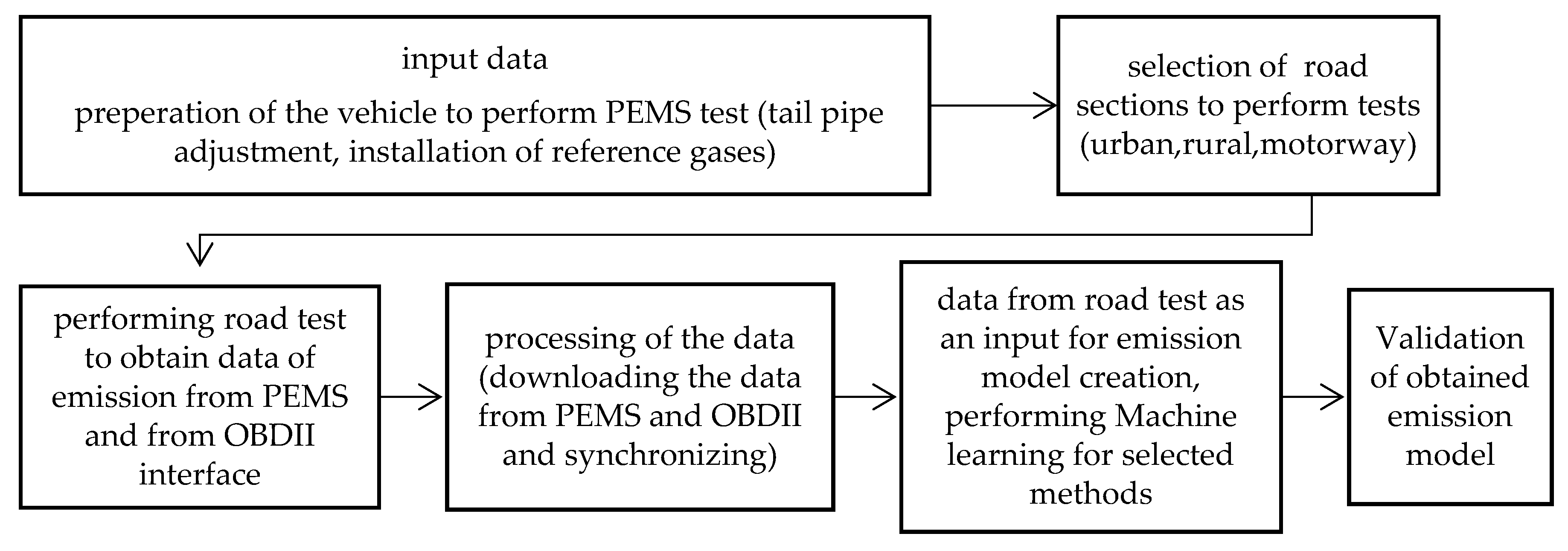
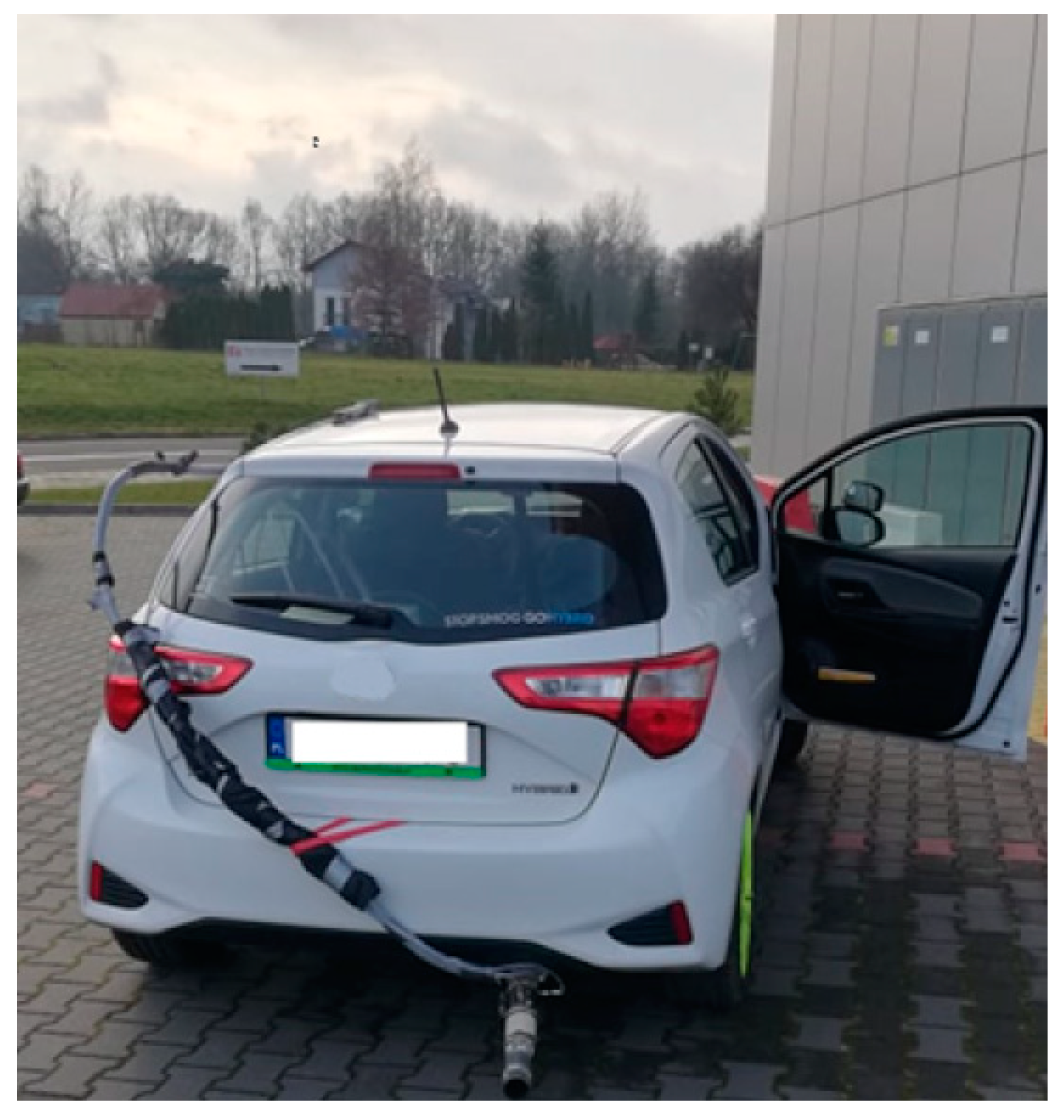
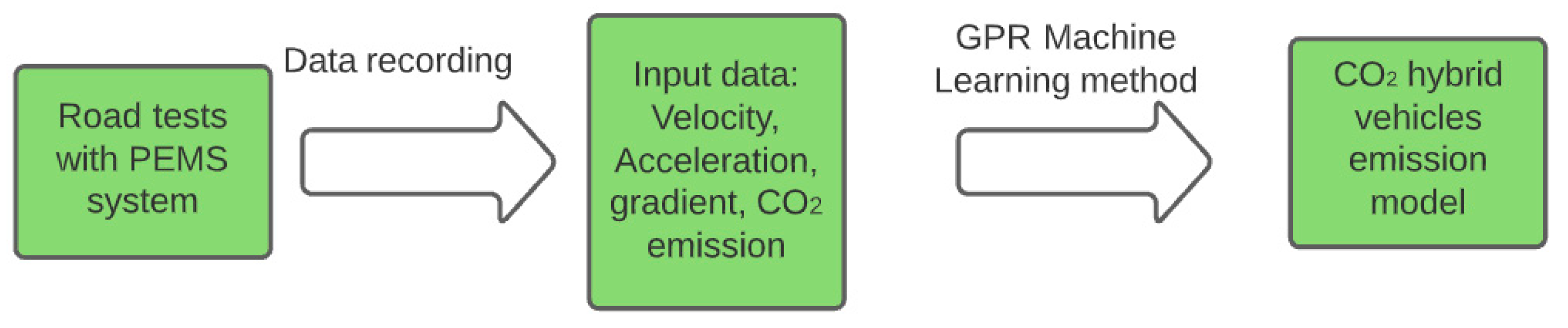
3. Methodology
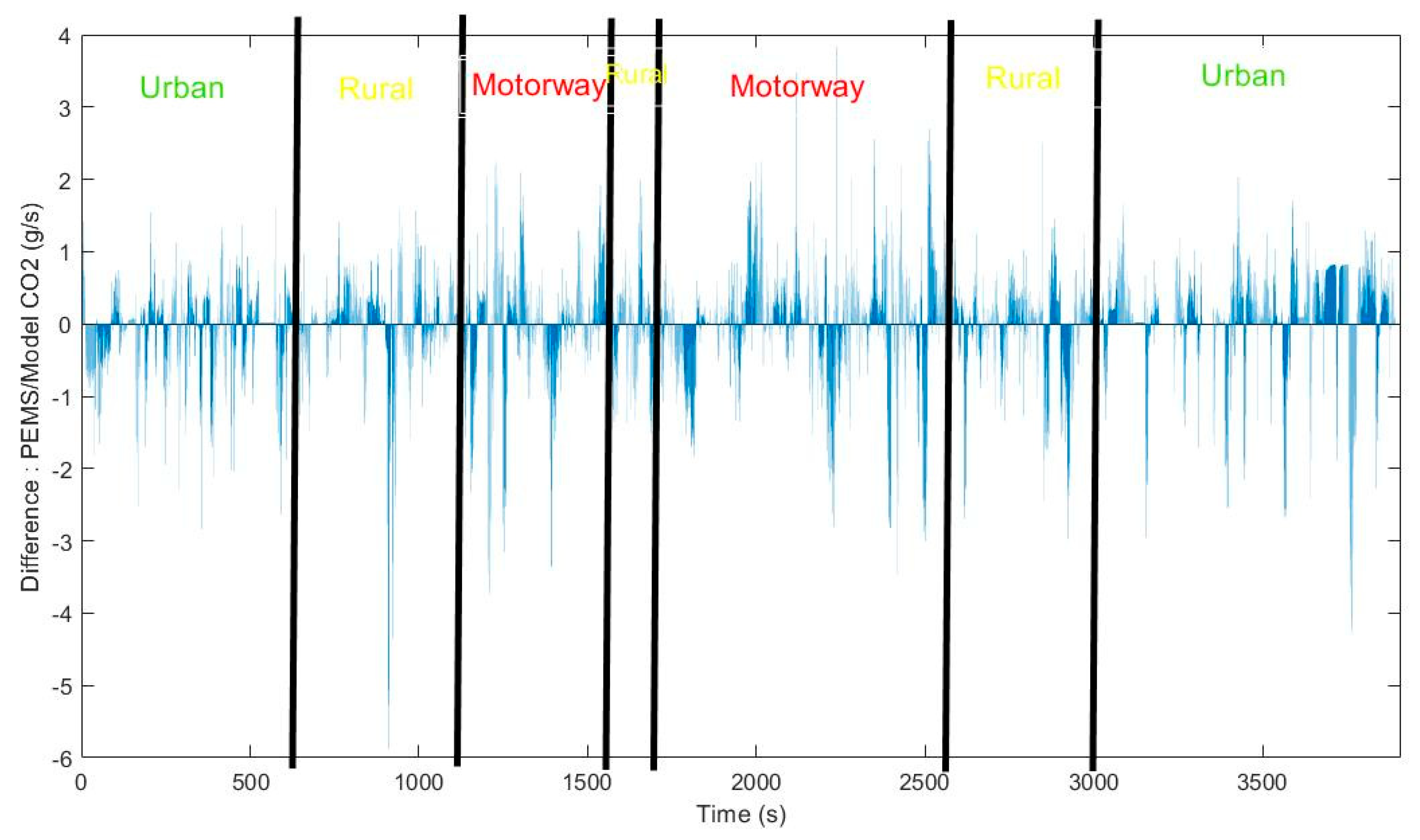
4. Results of Emission Model Validation
- n—number of samples,
- yt—forecast,
- —observed values.
- n—number of samples,
- yt—forecast,
- —observed values.
- R2—coefficient of determination,
- yt—forecast,
- —predicted values of the dependent variable,
- —average value of the actual dependent variable.
5. Conclusions
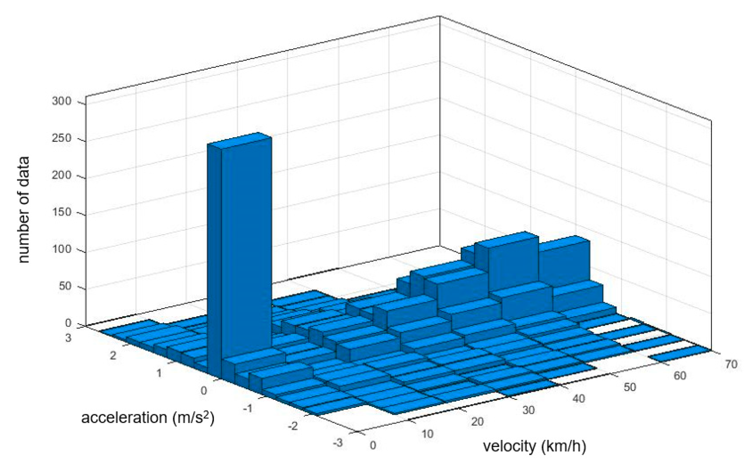
- CO2 emissions from hybrid vehicles are not strictly correlated with speed and acceleration because in some range of vehicle operation there is no emission, because combustion engine is not working.
- Machine learning methods are sufficiently sensitive to learn and create emission CO2 models for this kind of vehicle emission activities,
- Due to the variability of CO2 emission from the hybrid vehicle, there is a gap in the existing emission models, as they do not provide reliable results, especially when it comes to emission maps.
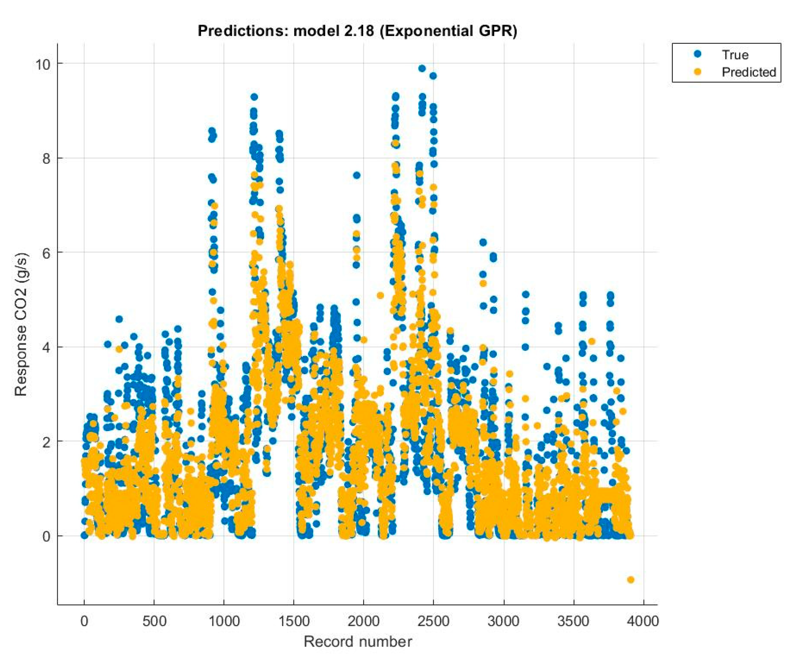
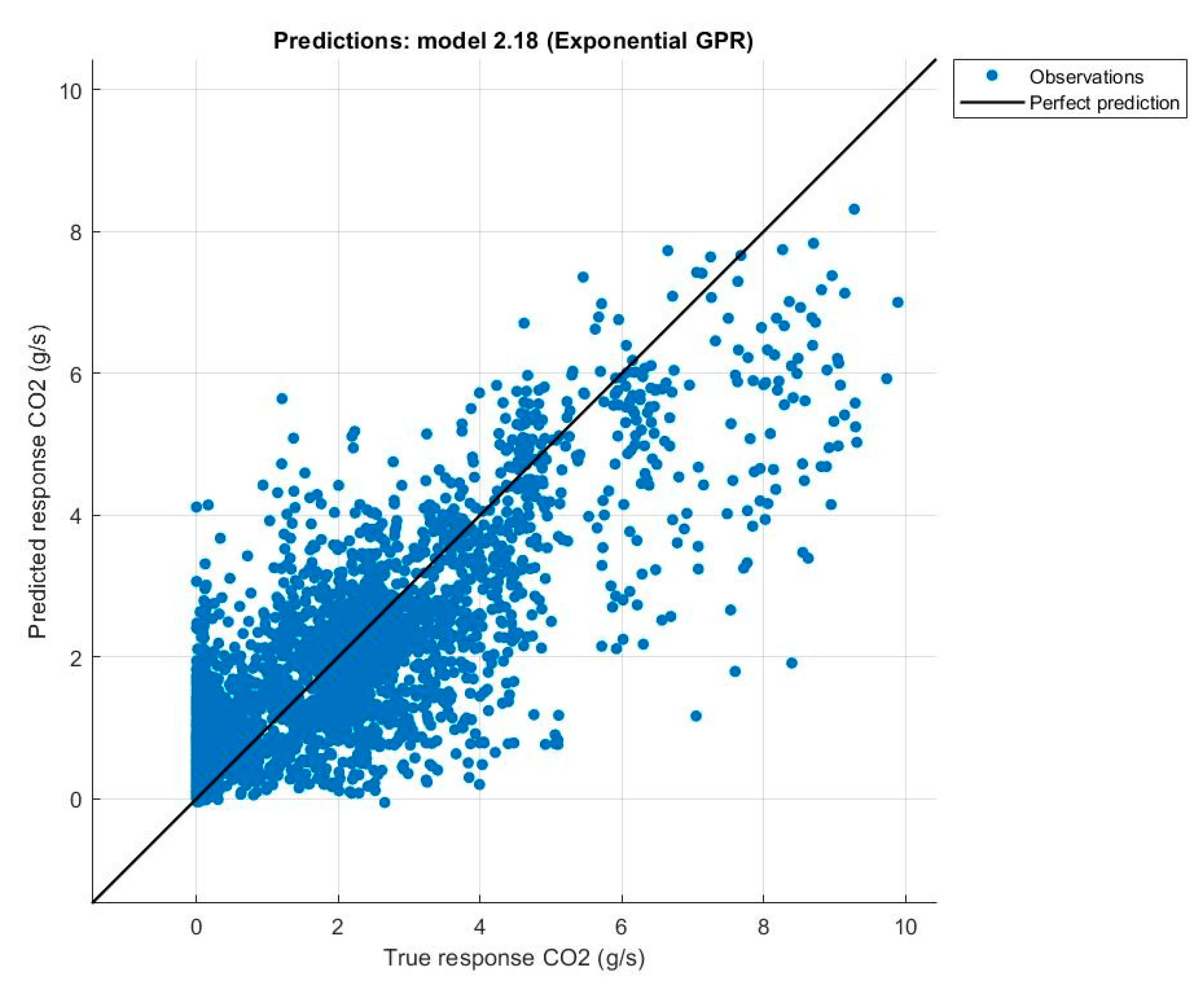
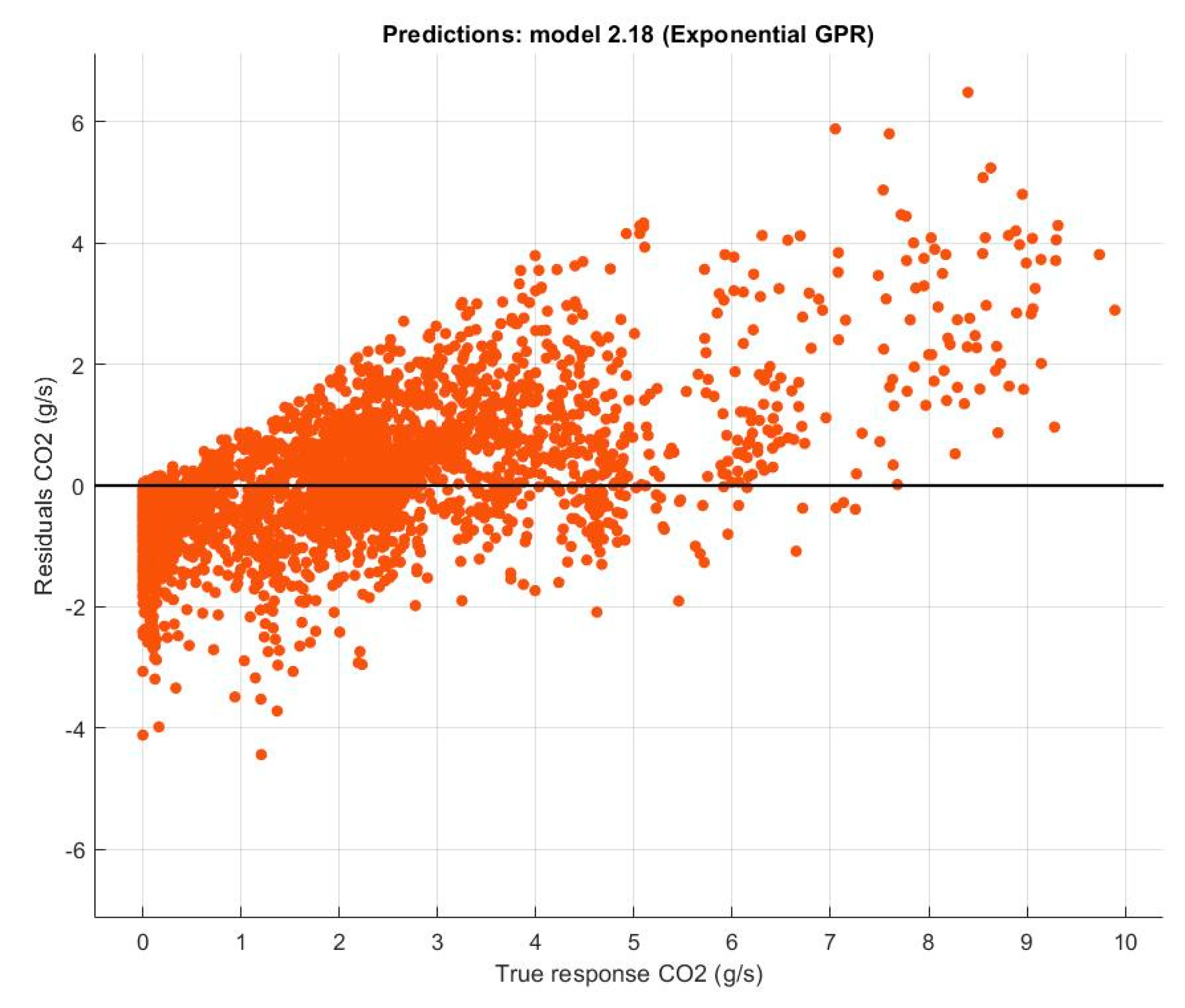
- Machine learning regression techniques can give an adequate emission model for full hybrid vehicles, especially for the Gaussian process regression technique.
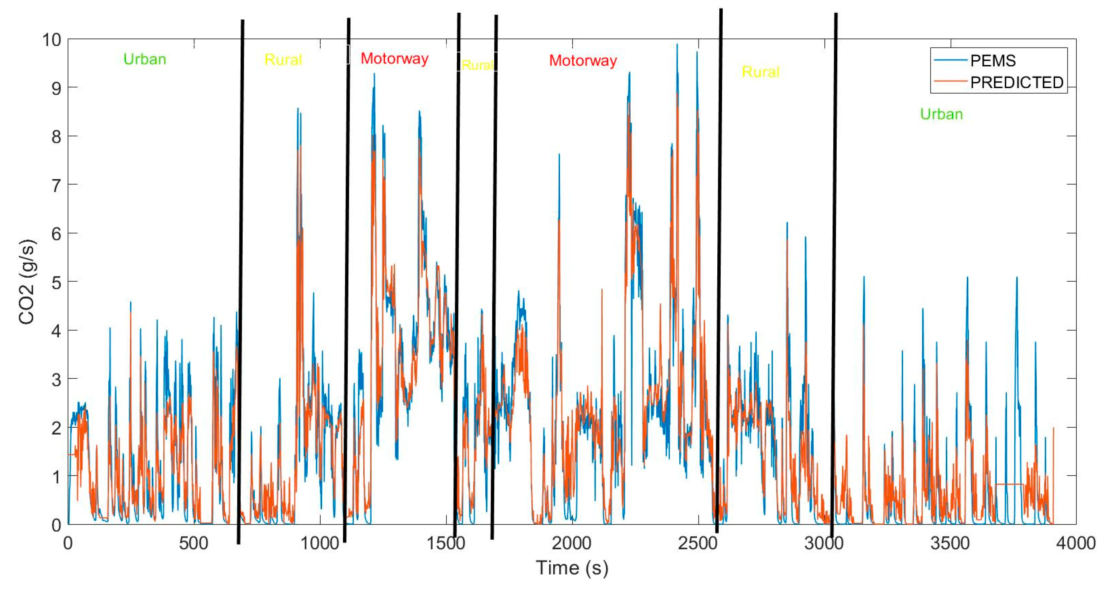
- The main issue of modelling CO2 emissions among hybrid vehicles touches urban roads, since there is the highest value and share of electric motor usage.
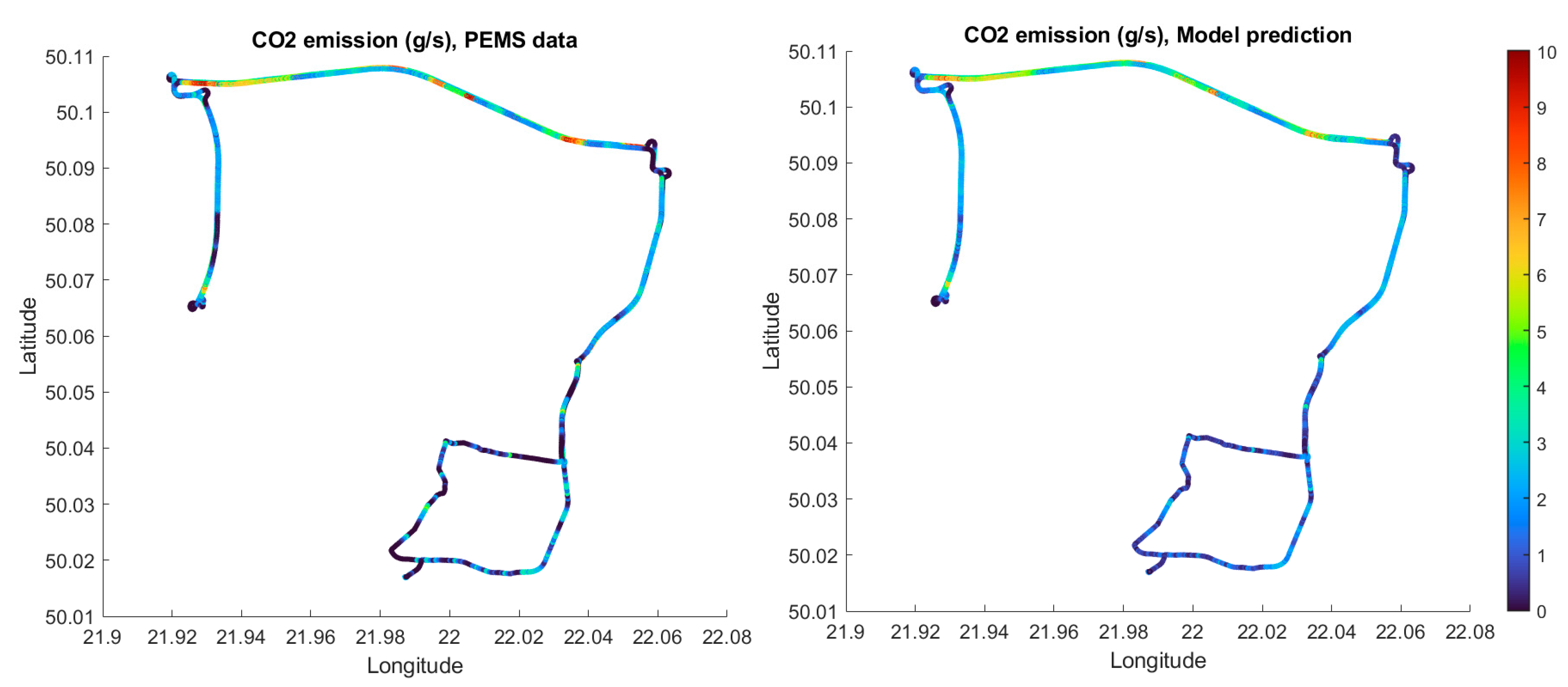
- The developed emission modelling methodology can be used in terms of microscale vehicle movement modeling to later create, for example, map on emission of researched part of the road to find zones with the lowest and highest CO2 emissions, and thus to develop more beneficial solutions to reduce these emissions.
Author Contributions
Funding
Institutional Review Board Statement
Informed Consent Statement
Data Availability Statement
Conflicts of Interest
Abbreviations
| CO | Carbon monoxide |
| CO2 | Carbon dioxide |
| GPR | Gaussian process regression |
| LPG | Liquified petroleum gas |
| MAE | Mean Absolute Error |
| MOE | Measures of effectiveness |
| MSE | Mean squared error |
| NNET | Neural network |
| NOx | Nitrogen oxides |
| PEMS | Portable Emission Measurement System |
| PHEV | Plug-in hybrid electric vehicle |
| PM | Particulate matter |
| R2 | Coefficient of determination |
| RMSE | Root mean square error |
| SVM | Support vector machine |
| THC | Total hydrocarbons |
References
- Tesoriere, G.; Campisi, T. The benefit of engage the “crowd” encouraging a bottom-up approach for shared mobility rating. In Proceedings of the International Conference on Computational Science and Its Applications, Cagliari, Italy, 1–4 July 2020; pp. 836–850. [Google Scholar]
- Acampa, G.; Campisi, T.; Grasso, M.; Marino, G.; Torrisi, V. Exploring European Strategies for the Optimization of the Bene-fits and Cost-Effectiveness of Private Electric Mobility. In Proceedings of the International Conference on Computational Science and Its Applications, Cagliari, Italy, 13–16 September 2021; pp. 715–729. [Google Scholar]
- Campisi, T.; Basbas, S.; Skoufas, A.; Akgün, N.; Ticali, D.; Tesoriere, G. The Impact of COVID-19 Pandemic on the Resilience of Sustainable Mobility in Sicily. Sustainability 2020, 12, 8829. [Google Scholar] [CrossRef]
- Caselli, F.; Grigoli, F.; Sandri, D.; Spilimbergo, A. Mobility under the covid-19 pandemic: Asymmetric effects across gender and age. IMF Econ. Rev. 2021, 2020, 1–34. [Google Scholar] [CrossRef]
- Ala, G.; Colak, I.; Di Filippo, G.; Miceli, R.; Romano, P.; Silva, C.; Valtchev, S.; Viola, F. Electric Mobility in Portugal: Current Situation and Forecasts for Fuel Cell Vehicles. Energies 2021, 14, 7945. [Google Scholar] [CrossRef]
- New Vehicle Registrations in the Fourth Quarter of 2020 Information. 2021. Available online: https://www.acea.auto/ (accessed on 2 October 2021).
- Noland, R.B.; Quddus, M. Flow improvements and vehicle emissions: Effects of trip generation and emission control technology. Transp. Res.-D 2006, 11, 1–14. [Google Scholar] [CrossRef] [Green Version]
- Smit, R.; Ntziachristos, L.; Boulter, R. Validation of road vehicle and traffic emission models—A review and meta-analysis. Atmos. Environ. 2010, 44, 2943–2953. [Google Scholar] [CrossRef]
- Mądziel, M.; Campisi, T.; Jaworski, A.; Kuszewski, H.; Woś, P. Assessing Vehicle Emissions from a Multi-Lane to Turbo Roundabout Conversion Using a Microsimulation Tool. Energies 2021, 14, 4399. [Google Scholar] [CrossRef]
- Elst, D.; Smokers, R.; Koning, J. Evaluation of the Capabilities of On-Board Emission Measurement System for the Porpose of Generating Real-Life Emission Factors; TNO Report; TNO Innovation for Life: The Hague, The Netherlands, 2004. [Google Scholar]
- John, C.; Friedrich, R.; Staehelin, J.; Schlapfer, K.; Stahel, W.A. Comparison of emission factors for road traffic from a tunnel study and from emission modeling. Atmos. Environ. 1999, 33, 3367–3376. [Google Scholar] [CrossRef]
- Kuhns, H.; Mazzoleni, C.; Mossmuller, H.; Nikolc, D.; Keislar, R.; Barber, P.; Zheng, L.; Etyemezian, V.; Watson, J. Remote sensing of PM, NO, CO and HC emission factors for on-road gasoline and diesel engine vehicle in Las Vegas, NV. Sci. Total Environ. 2004, 322, 123–137. [Google Scholar] [CrossRef]
- Merkisz, J.; Rymaniak, Ł. The assessment of vehicle exhaust emissions referred to CO2 based on the investigations of city bus-es under actual conditions of operation. Eksploat. I Niezawodn.–Maint. Reliab. 2017, 19, 522–529. [Google Scholar] [CrossRef]
- Yang, F.; Yu, L. A Microscopic Emission Model for the Light-Duty Vehicles Based on PEMS Data. In Proceedings of the Proceedings of International Conference of Transportation Engineering, Chengdu, China, 22–24 July 2007. [Google Scholar]
- Mądziel, M.; Campisi, T.; Jaworski, A.; Tesoriere, G. The Development of Strategies to Reduce Exhaust Emissions from Passenger Cars in Rzeszow City—Poland. A Preliminary Assessment of the Results Produced by the Increase of E-Fleet. Energies 2021, 14, 1046. [Google Scholar] [CrossRef]
- Song, G.; Yu, L.; Zhang, X. Emission analysis of toll station area in Beijing with portable emission measurement system. Transp. Res. Rec. J. Transp. Res. Board 2008, 258, 106–114. [Google Scholar] [CrossRef]
- Liu, H.; Barth, M.; Scora, G.; Davis, N.; Lents, J. Using portable emission measurement system for transportation emissions stud-ies: Comparison with laboratory methods. In Proceedings of the 86th Annual Meeting of the Transportation Research Board, Washington, DC, USA, 21–25 January 2010. [Google Scholar]
- Jaworski, A.; Mądziel, M.; Kuszewski, H.; Lejda, K.; Balawender, K.; Jaremcio, M.; Jakubowski, M.; Woś, P.; Lew, K. The Impact of Driving Resistances on the Emission of Exhaust Pollutants from Vehicles with the Spark Ignition Engine Fuelled with Petrol and LPG; SAE Technical Papers No. 2020-01-2206; SAE: Warrendale, PA, USA, 2020. [Google Scholar] [CrossRef]
- Merkisz, J.; Pielecha, J.; Bielaczyc, P.; Woodburn, J.; Szalek, A. A Comparison of Tailpipe Gaseous Emissions from the RDE and WLTP Test Procedures on a Hybrid Passenger Car; SAE Technical Papers 2020-01-2217; SAE: Warrendale, PA, USA, 2020. [Google Scholar] [CrossRef]
- Tran, M.-K.; Akinsanya, M.; Panchal, S.; Fraser, R.; Fowler, M. Design of a Hybrid Electric Vehicle Powertrain for Performance Optimization Considering Various Powertrain Components and Configurations. Vehicles 2021, 3, 20–32. [Google Scholar] [CrossRef]
- Madziel, M.; Jaworski, A.; Savostin-Kosiak, D.; Lejda, K. The Impact of Exhaust Emission from Combustion Engines on the Environment: Modelling of Vehicle Movement at Roundabouts. Int. J. Automot. Mech. Eng. 2020, 17, 8360–8371. [Google Scholar] [CrossRef]
- Zegeye, S.; Schutter, B.; Hellendoorn, J.; Breunesse, E.; Hegyi, A. Integrated macroscopic traffic flow, emission, and fuel con-sumption model for control purposes. Transp. Res. Part C 2013, 31, 158–171. [Google Scholar] [CrossRef]
- Quaassdorff, C.; Borge, R.; Pérez, J.; Lumbreras, J.; de la Paz, D.; de Andrés, J.M. Microscale traffic simulation and emission estimation in a heavily trafficked roundabout in Madrid (Spain). Sci. Total Environ. 2016, 566, 416–427. [Google Scholar] [CrossRef] [PubMed]
- Ahn, K.; Rakha, H.; Trani, A.; Van Aerde, M. Estimating vehicle fuel consumption and emissions based on instantaneous speed and acceleration levels. J. Transp. Eng. 2002, 128, 182–190. [Google Scholar] [CrossRef]
- Zhai, Z.; Tu, R.; Xu, J.; Wang, A.; Hatzopoulou, M. Capturing the Variability in Instantaneous Vehicle Emissions Based on Field Test Data. Atmosphere 2020, 11, 765. [Google Scholar] [CrossRef]
- Biggs, D.C.; Akcelik, R. An energy related model of instantaneous fuel consumption. Traffic Eng. Control 1986, 27, 320–325. [Google Scholar]
- Li, F.; Zhuang, J.; Cheng, X.; Li, M.; Wang, J.; Yan, Z. Investigation and Prediction of Heavy-Duty Diesel Passenger Bus Emissions in Hainan Using a COPERT Model. Atmosphere 2019, 10, 106. [Google Scholar] [CrossRef] [Green Version]
- Schnieder, M.; Hinde, C.; West, A. Sensitivity Analysis of Emission Models of Parcel Lockers vs. Home Delivery Based on HBEFA. Int. J. Environ. Res. Public Health 2021, 18, 6325. [Google Scholar] [CrossRef] [PubMed]
- Perugu, H. Emission modelling of light-duty vehicles in India using the revamped VSP-based MOVES model: The case study of Hyderabad. Transp. Res. Part D Transp. Environ. 2019, 68, 150. [Google Scholar] [CrossRef]
- Hamza, K.; Chu, K.-C.; Favetti, M.; Benoliel, P.K.; Karanam, V.; Laberteaux, K.P.; Tal, G. Comparisons of Real-World Vehicle Energy Efficiency with Dynamometer-Based Ratings and Simulation Models. World Electr. Veh. J. 2021, 12, 161. [Google Scholar] [CrossRef]
- Dong, Y.; Xu, J.; Liu, X.; Gao, C.; Ru, H.; Duan, Z. Carbon Emissions and Expressway Traffic Flow Patterns in China. Sustainability 2019, 11, 2824. [Google Scholar] [CrossRef] [Green Version]
- Lejri, D.; Can, A.; Schiper, N.; Leclercq, K. Accounting for traffic speed dynamics when calculating COPERT and PHEM pollutant emissions at the urban scale. Transp. Res. Part D Transp. Environ. 2018, 63, 588. [Google Scholar] [CrossRef] [Green Version]
- Emissions from Traffic Model Description. 2021. Available online: http://www.cerc.co.uk/environmental-software/EMIT-tool.html (accessed on 2 September 2021).
- Jaworski, A.; Mądziel, M.; Lejda, K. Creating an emission model based on portable emission measurement system for the purpose of a roundabout. Environ. Sci. Pollut. Res. 2019, 26, 21641. [Google Scholar] [CrossRef] [Green Version]
- Cornec, C.; Molden, N.; Reeuwijk, M.; Stettler, M. Modelling of instantaneous emissions from diesel vehicles with a special focus on NOx: Insights from machine learning techniques. Sci. Total Environ. 2020, 737, 139625. [Google Scholar] [CrossRef] [PubMed]
- Chen, G.; Wang, W.; Xue, Y. Identification of Ship Dynamics Model Based on Sparse Gaussian Process Regression with Similarity. Symmetry 2021, 13, 1956. [Google Scholar] [CrossRef]
- Varella, R.A.; Giechaskiel, B.; Sousa, L.; Duarte, G. Comparison of Portable Emissions Measurement Systems (PEMS) with Laboratory Grade Equipment. Appl. Sci. 2018, 8, 1633. [Google Scholar] [CrossRef] [Green Version]
- Ko, S.; Park, J.; Kim, H.; Kang, G.; Lee, J.; Kim, J.; Lee, J. NOx Emissions from Euro 5 and Euro 6 Heavy-Duty Diesel Vehicles under Real Driving Conditions. Energies 2020, 13, 218. [Google Scholar] [CrossRef] [Green Version]
- Pielecha, J.; Skobiej, K.; Kurtyka, K. Exhaust Emissions and Energy Consumption Analysis of Conventional, Hybrid, and Electric Vehicles in Real Driving Cycles. Energies 2020, 13, 6423. [Google Scholar] [CrossRef]


| Scale | Emission Model | Description |
|---|---|---|
| macro | Computer Program to Calculate Emissions from Road Transport (COPERT) | EU standard vehicle emission calculator. It uses vehicle mileage, speed etc. [27] |
| Handbook Emission Factors for Road Transport (HBEFA) | Application providing emission factor for different vehicle class [28] | |
| Motor Vehicle Emissions Simulator (MOVES) | Estimates emission for mobile sources at national, project and country scale [29] | |
| Emission Factors Model (EMFAC) | Computer model to estimate emission rate from motor vehicles for years 2000 to 2050 [30] | |
| micro | Comprehensive Modal Emission Model (CMEM) | Power-demand model based on a parameterized analytical representation of emissions production [31] |
| Passenger Car and Heavy-Duty Emission Model (PHEM) | Instantaneous vehicle emission model developed by the TU Graz covering different type of vehicles [32] | |
| Emissions from Traffic (EMIT) | Emissions calculations across large urban areas for dispersion modelling, allows to predict the impact of e.g., low emission zones [33] | |
| RoundaboutEM | Emission calculation from passenger cars for roundabout journeys [34] |
| Parameter | Data |
|---|---|
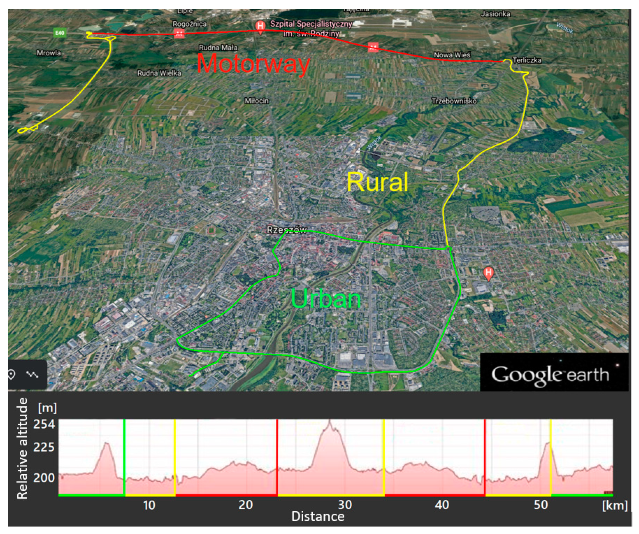
| Total distance (km) | 55.79 |
| Distance of the urban part (km) | 16.10 |
| Distance of the rural part (km) | 19.88 |
| Distance of the motorway part (km) | 19.81 |
| Average speed (km/h) | 55.29 |
| Urban average speed (km/h) | 32.56 |
| Rural average speed (km/h) | 62.24 |
| Motorway average speed (km/h) | 102.76 |
| Type of Model | RMSE (Validation) | R2 (Validation) | MSE (Validation) | MAE (Validation) |
|---|---|---|---|---|
| Tree, Fine tree | 1.1813 | 0.59 | 1.3955 | 0.71621 |
| Tree, Medium Tree | 1.2422 | 0.55 | 1543 | 0.8211 |
| Tree, Coarse Tree | 1.3053 | 0.51 | 1.7039 | 0.89876 |
| Linear Regression (linear) | 1.3948 | 0.43 | 1.9454 | 1.0258 |
| Linear Regression (Robust Linear) | 1.4189 | 0.42 | 2.0133 | 1.0026 |
| Stepwise Linear Regression | 1.3632 | 0.46 | 1.8584 | 0.99398 |
| Linear SVM | 1.4232 | 0.41 | 2.0256 | 1002 |
| Cubic SVM | 1.3524 | 0.47 | 1.8289 | 0.87705 |
| Esemble, Bagged Trees | 1.1929 | 0.59 | 1.423 | 0.8447 |
| Gaussian Process Regression (Exponential GPR) | 1039 | 0.69 | 1.0795 | 0.7066 |
| Neural Network (Three-layered Neural Network) | 1.2559 | 0.54 | 1.5773 | 0.87841 |
Publisher’s Note: MDPI stays neutral with regard to jurisdictional claims in published maps and institutional affiliations. |
© 2021 by the authors. Licensee MDPI, Basel, Switzerland. This article is an open access article distributed under the terms and conditions of the Creative Commons Attribution (CC BY) license (https://creativecommons.org/licenses/by/4.0/).
Share and Cite
Mądziel, M.; Jaworski, A.; Kuszewski, H.; Woś, P.; Campisi, T.; Lew, K. The Development of CO2 Instantaneous Emission Model of Full Hybrid Vehicle with the Use of Machine Learning Techniques. Energies 2022, 15, 142. https://doi.org/10.3390/en15010142
Mądziel M, Jaworski A, Kuszewski H, Woś P, Campisi T, Lew K. The Development of CO2 Instantaneous Emission Model of Full Hybrid Vehicle with the Use of Machine Learning Techniques. Energies. 2022; 15(1):142. https://doi.org/10.3390/en15010142
Chicago/Turabian StyleMądziel, Maksymilian, Artur Jaworski, Hubert Kuszewski, Paweł Woś, Tiziana Campisi, and Krzysztof Lew. 2022. "The Development of CO2 Instantaneous Emission Model of Full Hybrid Vehicle with the Use of Machine Learning Techniques" Energies 15, no. 1: 142. https://doi.org/10.3390/en15010142
APA StyleMądziel, M., Jaworski, A., Kuszewski, H., Woś, P., Campisi, T., & Lew, K. (2022). The Development of CO2 Instantaneous Emission Model of Full Hybrid Vehicle with the Use of Machine Learning Techniques. Energies, 15(1), 142. https://doi.org/10.3390/en15010142