Abstract
The European Union aims to reduce Greenhouse Gas (GHG) emissions by 55% before 2030 compared to 1990 as a reference year. One of the main contributions to GHG emissions comes from the household sector. This paper shows that the household sector, when organised into a form of prosumer microgrids, including renewable sources for electric, heating and cooling energy supply, can be efficiently decarbonised. This paper investigates one hypothetical prosumer microgrid with the model RES2GEO (Renewable Energy Sources to Geothermal). The aim is to integrate a carbon-free photovoltaic electricity source and a shallow geothermal reservoir as a heat source and heat sink during the heating and cooling season. A total of four cases have been evaluated for the Zagreb City location. The results represent a balance of both thermal and electric energy flows within the microgrid, as well as thermal recuperation of the reservoir. The levelised cost of energy for all cases, based on a 20-year modelling horizon, varies between 41 and 63 EUR/MWh. On the other hand, all cases show a decrease in CO2 emissions by more than 75%, with the best case featuring a reduction of more than 85% compared to the base case, where electricity and gas for heating are supplied from the Distribution System Operator at retail prices. With the use of close integration of electricity, heating and cooling demand and supply of energy, cost-effective decarbonisation can be achieved for the household sector.
1. Introduction
Reduction of environmental pollution while ensuring sustainable development has several key elements. The first stage is to diagnose the current state of industrial and residential systems via evaluation of resource use and released footprints [1]. The other elements also include appropriate targeting of the needs for heat and power supply [2], as well as targeting power generation operation for a given local grid [3]. For thermal applications, district heating and cooling systems in the European Union (28 countries) in 2019 reached an installed geothermal capacity of 5.5 GWth. Also, over 2 × 10⁶ geothermal heat pumps were installed in Europe as of June 2020 [4]. Sweden, Germany, France and Switzerland are countries with the most installations of shallow geothermal (SG) heat capture systems, accounting for 64% of all installed capacity in Europe [5]. Dalla Longa et al. [6] project that the geothermal energy heat production would reach around 100–210 TWh/y by 2050. Shallow geothermal energy in Croatia is relatively new, and the exploitation of its potential started around 2008 [7]. It is estimated that the total energy sourced by using SG energy in 2018 was 4.45 GWhth [8].
The ground heat exchanger is the main part of all SG energy systems. It is typically connected to the heat supply system via heat pumps. A heat transfer fluid may circulate through the ground heat exchanger in two ways. There are shallow horizontal systems, where pipes are placed near the ground surface and arranged in ditches. The second type of arrangement involves vertical boreholes of small diameter, which penetrate around 200 m in depth. Which of these two types will be used depends on ground thermal properties. Thermal testing of soil can be carried out in a laboratory or in situ. The most used in situ test type is the Thermal Response Test (TRT) [9], which measures the temperature response of the rock. Depending on the heating (and/or cooling) needs, TRT shows if the rocks can deliver the desired amount of energy. Over the years, the thermal output of rocks decreases [9]. Bu et al. [10] found that the average extracted thermal output during ten heating seasons reduces by 7.77%. The decrease can be smaller with the use of a cooling regime system during the summer, in which case the rocks can recover thermally. As a follow-up on that research, He and Bu [11] developed an enhanced deep borehole heat exchanger that allows more than doubling the heat extraction compared with the initial benchmark design.
During the production from shallow geothermal, the heat content decreases. The recovery process begins when production is complete. Natural forces, such as pressure and temperature gradients, drive the recovery. In the beginning, recovery is strong and slows over time. Theoretically, the original state will be re-established after an infinite amount of time.
According to [12], reservoir recovery depends on the purpose of the shallow geothermal reservoir. If utilisation was only for electricity generation (high-enthalpy reservoir), 95% recovery of the original amount of heat will be reached after several hundred years; for district heating (doublet system) recovery of 95% takes approximately 100–200 years; and for a decentralised shallow HP system, time for 95% of recovery is approximately equal to the production time (e.g., 30 years of production needs 30 years of recovery).
Advanced heat recovery can be obtained via thermal battery storage with water as the medium. Seyam et al. [13] designed a hybrid energy system consisting of PV, geothermal loop (300 m length) and thermal battery storage with 9463.53 kg of water for heating (and cooling) residential buildings in Canada. The study showed that 9 kW of heating load could be provided with thermal battery storage to a condenser that increases the water temperature by 10 °C.
According to the World Bank [14], it is predicted that by 2030 almost 60% of the world population will live in urban areas, following the share of over 55% in 2019. A higher concentration of people means more intensive energy consumption. It is necessary to reduce the consumption of fossil fuels, especially in urban districts. The European Commission [15] has developed climate strategies and key targets for 2030, aiming to cut the greenhouse gas emissions by at least 40% from the 1990 levels by achieving at least 32% share for renewable energy and at least 32.5% improvement in energy efficiency.
To fulfil those targets, it is necessary to plan new urban areas and reconstruct existing ones in a way that includes usage of various renewable energy sources—allowing for combinations. Shallow geothermal energy, combined with solar photovoltaics (PV) (with or without battery), is one of the promising solutions. Schiel et al. [16] developed a method for utilising SG energy for space heating and hot water using a single borehole for lower heating energy demands in residential applications. Using Geographical Information Systems (GIS) can help to identify areas with high intensity of solar insolation that can be suitable for such an energy mix. That idea was further used by Walch et al. [17] for developing a method for quantification of the technical potential of shallow geothermal sources at a regional scale, as well as by Ramos-Escudero et al. [18]—already to the continental scale of Europe.
Microgrids are energy network arrangements [19] that can enable providing a suitable renewable energy mix [20] for serving residential demands—including for geothermal-based heat pumps. A microgrid forms a cluster of load demands and micro-scale power sources (<100 kW) operating as a single controllable system capable of providing both power and heat to its local area [21]. Power can be generated by solar panels, wind turbines, Combined Heat and Power [22]. Newer microgrids have energy storage, typically consisting of electrical batteries, and can also have electric vehicle charging stations [23].
As of 2015, the world leader in installed microgrid capacity [24] is China, with 153 GW in 2014. In the European Union, Germany has an installed capacity of 85.8 GW, Italy 32.1 GW and Spain 31.7 GW. No specific regulations and policies are formulated on the utilisation and deployment of distributed energy generation and microgrids in the EU.
Geothermal energy is utilised via wells of various depths and different arrangements of the operating units. According to [25], the systems are based on the following classifications:
- Depth of the geothermal reservoir: shallow (<300–500 m), intermediate (<3–5 km), deep (further depth levels);
- Generation type: power generation, direct heat use, geothermal heat pumps.
Vieira et al. [26] have investigated the thermal and mechanical properties of soil. They developed an experimental procedure following steady-state and transient methods, comparing the results. The authors reported significant differences between laboratory and field-testing results, concluding that further developments are necessary for constructing reliable parameter identification methods.
For making regional and infrastructure-related decisions, mapping the shallow-geothermal heat potential is very important. A general method for performing this activity has been published by Casasso and Sethi [27]. They have illustrated the method on the SG mapping of the Piemonte region in Italy, identifying up to 12 MWh/y heat extraction potential from boreholes in the plain part of the region. That work follows up on a more thorough study from 2007 [28] that has studied the geographical potential for SG heat exploitation, which explores the depth alongside the surface coordinates as factors. A mapping of the available SG potential for the city of Vienna has been recently published [29]. The authors reported that up to 63% of the city heating demand could be covered by the available potential. No specific heat flows or temperatures are quoted in the article, but a link to the raw data sets is provided. Those works have been complemented by an updated database [30] of ground thermal properties for Ground Source Heat exchangers and Pumps from European regions—including Italy, Croatia, Germany.
A thorough review of the state of the problems and the legislation in selected countries have been performed by Somogyi et al. [31]. They have suggested the development of a unified methodology for the assessment of SG systems on an enthalpy basis. A major conclusion of the study is that the legislation generally lags significantly behind the research results and not taking advantage of them, accompanied by a lack of a systematic regulation (as of the time of publication). An interesting finding is that only German regulations required numerical assessment for proving the design credibility. The suggested technology development options also include the use of solar heat for the regeneration of the heat content of the ground.
Cai et al. [32] presented and demonstrated an analytical model for predicting the thermal response in boreholes with groundwater advection. The model was validated and demonstrated on case studies with various configurations, identifying tangible benefits from exploiting sites with multiple boreholes.
The feasibility evaluation of long-term intensive SG utilisation is described by Meng et al. [33]. The authors described a 24-year-long comprehensive investigation of joint exploitation of an SG heat source with multiple boreholes. They concluded that even intensive exploitation of the source is feasible for the long term, subject to variations in the efficiency of the installations in time and with the underground water flow direction. The performance deteriorated with time and stabilised, and downstream installations tend to get lower-temperature heat source. These concerns indicate the need to combine the SG heat source with a solar thermal capture installation for the restoration and rehabilitation of the ground heat source. Those results are corroborated by a shorter-term measurement study for the area of Cologne in Germany [34].
An evaluation of an SG energy source for combined heating and cooling applications in residential areas has been performed for the climate of Beijing [35]. The authors have developed an operating policy that allowed to extend the annual period without air conditioning by 34% and realise nearly 30% energy savings compared to a conventional ground-source heat pump system.
An interesting installation that increased the heat capture rate has been proposed by Sofyan et al. [36], exploiting a combined vertical-horizontal heat exchanger. The authors provided a comprehensive analysis of the possible operating policies. From that, the enhanced performance of the combined heat exchanger in a series mode that alternated horizontal and vertical parts operation achieved the highest heat transfer rate, which can be explained by allowing the surrounding soil to recover the thermal potential when one of the heat exchanger parts is out of operation.
The technical and cost performance change from improving the thermal properties of the borehole heat exchangers have been evaluated for a Croatian case study [37]—with a site located near the capital Zagreb. The evaluation reported that the enhancements are not beneficial. The main reason for this was found in the low thermal conductivity of the soil at the experimental site, and it was recommended to use thermal enhancement retrofits only for sites with soil conductivity above 2 W/(m × °C).
The long-term planning for safe operation also includes the evaluation and the optimisation of the reliability, availability and maintenance of the involved heat exchangers, as shown in [38]. The soil properties and the operation of the SG heat capture system are also closely related to the hydro-chemical properties of the groundwater [39]—especially the solubility of the various minerals and the potential for scaling. The authors of that study concluded that, at lower depths, scaling of Ca-ion salts is very likely.
Kljajić et al. [40] have evaluated the economic feasibility and the environmental performance of a potential district heating plant based on a shallow geothermal source. The case study site is from the north of Serbia. While the thermal and the economic performance of the considered geothermal exploitation system was positive, resulting in a payback period of 4.9 years, the Global Warming Potential and other indicators resulted in poor performance, e.g., the Greenhouse Gas emissions almost doubled, which is explained with the high share of coal in the Serbian grid electricity mix.
The review of the previous works reveals a pattern of tackling a wide spectrum of issues related to SG heat exploitation. These include the following:
- Evaluation of the soil properties for aiding the SG system design
- Regional mapping—by geographical coordinates and depth
- Evaluation of the regional potential to cover local heating needs
- Evaluation of the legislation and regulations across the EU
- Operational issues—evaluation of thermal SG capacity replenishment and deterioration of underground sites, dynamic operation planning using SG sites as heat storage
- Intensification of the SG heat extraction via innovative heat exchanger design and borehole design adjustment
- Maintenance and reliability issues related to scaling
- Techno-economic-environmental feasibility evaluation of SG for district heating with heat pumps.
These all are important issues, but their span and the published results clearly show a significant further scope for improved system design and operation. In this context, using solar thermal capture in combination with SG heat is an area that is still waiting for significant advances, while it has clearly a good potential for utilising renewables at an acceptable cost. Based on the analysis of the state-of-the-art, the current paper considers the evaluation of the design and operation of residential Combined Heat and Power (CHP) systems, offering one possible implementation of the concept of Total EcoSites [41], while maximising the utilisation of the captured solar and geothermal energy. The goal is to evaluate the technical feasibility and the economic viability of the system.
This working hypothesis is that the use of geothermal heat pumps in combination with renewable sources of electricity, such as PV, can be used for cost-effective decarbonisation of the energy consumption of the household sector. With the integration of heating, cooling and electricity demand and renewable supply, sustainable utilisation of the energy from the geothermal reservoir can also be achieved with the low year-to-year thermal degradation of the reservoir.
2. Materials and Methods
The overall method consists of the estimation of input data; calculation of heating, cooling and electricity demand for the residential microgrid; multi-year simulation of the microgrid with special emphasis on reservoir modelling and analysis of results. Input data also contains the inputs for techno-economic analysis. In this paper, the RES2GEO (Renewable Energy Sources to Geothermal) model is used for performing the system evaluation. This is an in-house model, written in Python v.3.8 [42] for the current work and presented in this section. The model takes as inputs the energy demands and environment parameters. As an output, it estimates the use of primary energy and costs—operating and investment. It can simulate multiple-year scenarios with sufficiently small time-steps, balancing both electricity and heat flows within the microgrid system. The scheme of the system is presented in Figure 1. The model is sufficiently detailed to incorporate variable power supply from renewable energy sources as input parameters and flexible heat production from shallow geothermal as an output parameter.
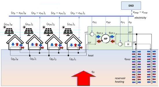
Figure 1.
Scheme of the microgrid system in RES2GEO model, DSO: Distribution System Operator.
The electricity and heat flows (supply and demand) are balanced on an hourly basis, assuming pseudo-steady-state, defining a set of time slices within a specified time horizon. The model considers the thermal inertia of the geothermal reservoir. While heating objects and water circulations are modelled as lumped-parameter systems, a reservoir is modelled as a distributed parameter system. The simulation time step is one-quarter of an hour, and the results are recorded every hour.
The coefficient of performance (COP) of the heat pump (HP) is modelled as a 2-nd order polynomial with formula according to Ecoforest heat pump technical data [43]:
where EST is Entering Source Temperature. During the heating period, EST is equal to the temperature of the water from a reservoir, as calculated by the reservoir model, and during the cooling period, it is assumed to be equal to 12 °C, i.e., this is return temperature from the cooling object. During the heating season, the primary circulation circuit is between the reservoir and the HP, and during the cooling season, the primary circuit is between the cooling object and HP. Energy demand from the pump between the heating/cooling object and the HP is neglected.
2.1. Modelling of a Shallow Geothermal Reservoir and a Borehole Heat Exchanger
The shallow geothermal reservoir is modelled as the concentric tubular shape that is axially symmetric. Axial symmetry allows us to model the reservoir as a cake slice, i.e., 2D slice (see Figure 2). The model is essentially a model with distributed parameters and coupled with the model of the surface equipment. The role of this model is to capture physical processes influenced by the thermal inertia of the reservoir. In a reservoir, temperature changes occur at a much slower time rate than changes in electricity and heat demand and solar insolation.
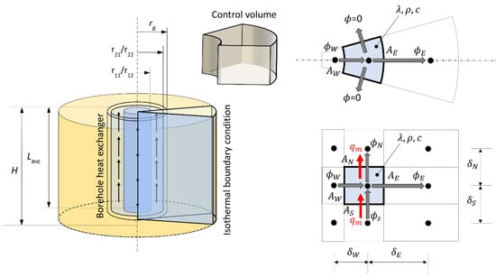
Figure 2.
Schematic view of the reservoir and coaxial borehole heat exchanger.
Every 2D cell represents a control volume in which a heat balance is calculated for every time step of the simulation. The heat balance states that time change of the energy contained in the cell equals a net change of the heat rate through the boundary of the cell (Equation (2)):
A positive heat rate denotes energy input, and a negative heat rate denotes an energy outlet from the cell. Following the notation from Figure 2, where the initial and assumed signs of heat rates are presented, the following equation can be written:
The balancing is done between the nodes of the cells that are positioned in the geometrical centre of the control volume of the cell. There are several types of control volumes in the reservoir and borehole heat exchanger. Control volume cells containing only solid matter are the ground itself, the grout and polyethene material of the coaxial borehole heat exchanger (BHE). Control volume cells containing the fluid flux are the tube (downward flow) and annulus (upward flow). Physical properties are assumed to be homogeneous within the control volumes but can differ between control volumes. In more detail, the upper equation can be written as follows:
The assumed positive sign of the heat flow and convective flow is presented in Figure 2. The convective part of the equation exists only in the control volume with the fluid flow streaming through it. These are control volumes in the downwards tube and upwards annulus as a part of the BHE. For the calculation of the overall heat transfer coefficient k, the thermal properties of each matter in the system have to be known. These are thermal conductivities λ, heat capacities c and densities ρ for the soil/rock, bentonite, polyethene and circulating water. Water is modelled as a perfectly incompressible fluid.
For the control volumes having both the convective and conductive part, the equation is as follows:
and for the cells having no convective flow, the previous equation takes the simpler form:
From Equations (5) and (6), it is seen that both the physical parameters of the matter and geometrical parameters of the control volume, i.e., the mesh, are influencing the results. The mesh is structured but not equidistant, and the mesh has to be sufficiently dense. Physical parameters of the reservoir have to be properly selected, meaning that thermal conductivity, specific heat capacity and density have to correspond to the specific location. Due to the depths of the BHE reaching approximately 100 m, the physical properties can be set to depend on the depth of the reservoir.
Equations can be written in the final form:
For each control volume, Equation (5) is set, and the resulting system of equations is calculated with the linear solver linalg, a submodule of NumPy library [42]. The boundary condition of the computational domain of the reservoir is Dirichlet-type and assumed to be isothermal. The heat exchange with the reservoir can be calculated from the equation balancing the heat flow between the boundary node and first node to the boundary:
2.2. Techno-Economic Analysis and Levelised Cost of Electricity and Heating Energy
In this paper, three types of cost are distinguished: Capital Expenditures (CAPEX), Operating Expenses (OPEX) and capital cost. CAPEX cost is a derived indicator that tracks the annual payments on the total investment cost, multiplied by private equity. Investment and CAPEX can be calculated from the equations:
A loan can be defined as the rest of the CAPEX cost:
The loan is a part of the OPEX that is covered by the bank and therefore generates the additional cost. Time series of principal and interest for a year i can be defined from PPMT (Principal Payment) and IPMT (Interest Payment) Excel functions:
The cost of capital is the total sum of interest payments over the years.
OPEX cost is the cost of imported electricity:
where the price of electricity is escalated over the years:
The cumulative cost over the years can be obtained by summing up all discounted costs over the years:
Levelized cost of energy (LCOE) is, by definition, calculated as discounted costs divided by the discounted energy, summed up for a period of equipment lifetime or any other reasonable time horizon. In this paper, both the electricity and heating energy is discounted for a period of 20 y with a predetermined discount rate d. LCOE is calculated with the formula:
Energy demand is consisting of electricity, thermal and cooling demand. Since it is not possible to distinguish the costs related solely to the cost of electricity and heat, a single value of LCOE is calculated.
3. Setup of the Hypothetical Case Study
The case study represents a small residential area consisting of 20 houses. Each house has a floor area of 250 m2. The heat demand is calculated based on the outside temperature data for the year 2016 for Zagreb. Both electricity and heat demands are aggregated over the twenty residential objects.
The estimation of the hourly heat demand (net heat flux), is based on the normalised distribution of the difference between the indoor temperature Tindoor and the outdoor temperature Toutdoor, the total residential area Atot and annual heat demand in kWh/m2. The algorithm is based on a report from the Heat Roadmap Europe project Stratego [44] and is presented in the Supplementary Materials. The solution provides values of net heat flux from heating and cooling . The heating period is 7 a.m.–7 p.m. Heating is switched on if the temperature drops below 20 °C and off if the indoor temperature rises above 24 °C. Cooling is switched on at indoor temperature above 26 °C and off below 22 °C. Outside of the heating period, heating is switched on if the temperature drops below 14 °C, and switched off if the indoor temperature rises above 18 °C. The heating and cooling demands can be derived from the net heat flux with simple relations (Equation (20)).
The outdoor temperature was estimated using the platform for obtaining the energy input data for PV—the Photovoltaic Geographical Information System (PVGIS) version 5 [45]. Annual heat demand per unit area is set to the value of 50 kWh/m2. The resulting temperature profiles and heating/cooling demands are shown in Figure 3. All results are presented for a period between 1st of April and 30th of March, with data taken as periodic timeseries data based on Year 2016.
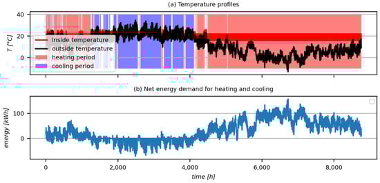
Figure 3.
Temperature profiles and the resulting net heat fluxes; the plot for net heat flux is convoluted with the band of 8 h.
It is assumed that the system has a ceiling heating/cooling facility. Figure 3a shows the temperature profiles of the interior and outside air, with heating and cooling periods shaded in red and blue. The heating demand is approximately ten times larger than the cooling, which indicates that the regeneration of the reservoir temperature during the cooling season cannot be done simply with heat rejection from the cooling object. Additional heating from the electric heater can be used to recover the reservoir temperature during periods with excess power from the PV system. Figure 3b represents the net heat balance of the interior air and the wall, that is an input to the energy balance. Positive values indicate heating demands, and negative values indicate cooling demands.
The electricity demand for a single house is plotted in Figure 4, reflecting peak demands. It is estimated by using the superposition of random bimodal distribution around two peaks of 7 a.m. and 7 p.m. and variances equal to two. The electricity demand used as an input to the model is demand from all appliances, excluding the electricity needed to run heat pumps, pumps and electric heaters.
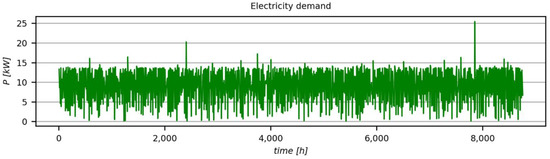
Figure 4.
Electricity demand for one year; the plot is convoluted with a band of 8 h.
The total energy demand of the microgrid is presented in Table 1. That includes all houses in the microgrid by categories: heating, cooling and electricity demand, without electricity demands which are part of the systems for heating and cooling, like heat pumps, electric heaters and pumps. Heating demand is almost three times larger than electricity demand and more than 10 times larger than cooling thermal demand.

Table 1.
Energy demand parameters for the microgrid.
The distribution of the production from the PV for the Zagreb area (Figure 5) is taken from PVGIS 45 PV performance interactive tool. Mounting type is fixed with optimised slope and azimuth angles and PVGIS-SARAH solar radiation database.
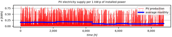
Figure 5.
Distribution of PV electricity energy supply per 1 kW-peak of installed power.
The curtailment of the PV system is allowed, and all electricity produced from PV must be utilised in the microgrid, exported to the grid or curtailed if there is no option to use it or to export it. The net metering on an annual basis must be positive:
The actual production of the energy from the PV is obtained from multiplying the unit distribution with the nominal power of the PV. The levelised cost of energy was calculated with the following assumptions: 6% discount rate, 3% cost of capital, 10 y capital loan, 20% equity. The subsidy is fixed at 2500 EUR, the cost of wells are 46 EUR/m, and all wells are at 100 m of depth. The overnight cost of the project is 4000 EUR, and the installation cost is 65,000 EUR. The cost of equipment is: PV system is 790 EUR/kW, heat pump 660 EUR/kW, electric heater 131 EUR/kW and the pump is 530 EUR/kW.
4. Results and Discussion
4.1. Preliminary Testing
Due to the large number of possible system design combinations, the one-year simulations have been performed initially to estimate the optimal configuration with respect to the minimum overall discounted cost Cd and minimum annual change in temperature of the reservoir ΔT. Design variables under consideration are installed PV power, installed heater power and the number of shallow geothermal wells. All three variables increase the CAPEX cost and cost of capital and decrease the OPEX cost. A total of 125 single-year simulations have been performed, and the feasible solutions are presented in Figure 6.
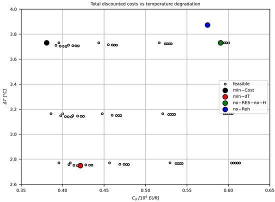
Figure 6.
Discounted costs vs. temperature difference in a shallow geothermal reservoir for all system designs; unfeasible designs are marked with crosses and feasible with circles.
Two feasible optima can be observed: the first one for the minimum discounted cost, the min-Cost case, and the second one for a minimum degradation in reservoir temperature, the min-dT case. For the reference point, the scenario with no heater and PV, the no-RES-no-H case, as well as the case not including the reheat at all, the no-Reh case, are also analysed. All four cases are summarised in Table 2.
Table 2.
Four selected cases for further investigation.
With the four selected cases, separate individual long-term simulations with a 20-year time horizon have been performed. For these cases, a detailed technical and, together with techno-economic analysis, is presented.
4.2. Time Series Analysis for the Selected Cases
Time-series analysis of the four selected cases, Table 2, is used to analyse the energy flows. For the twentieth (20) year of the simulation, the time series and total annual energy flows are presented in Figure 7 and Figure 8. Input data for all long-term simulations are taken as periodic timeseries data input based on Year 2016 and all results are presented for a period between 1st of April and 30th of March.
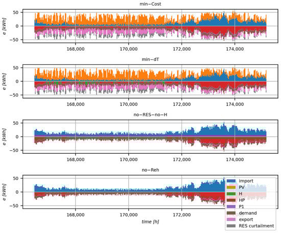
Figure 7.
Energy balance in the last simulation year for all selected cases.
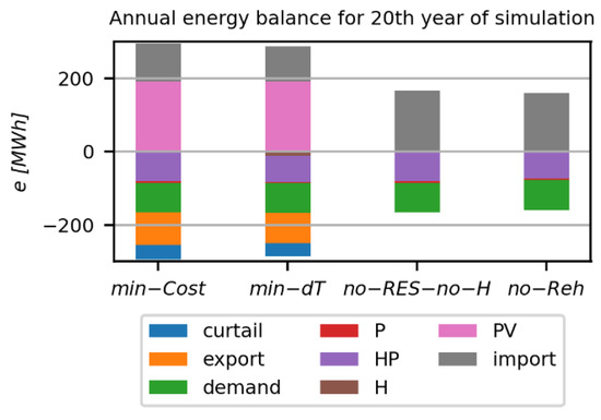
Figure 8.
Decomposition of annual energy flow in the last (20th) simulation year.
In cases min-Cost and min-dT, the curtailment of the PV-power can be seen. Energy flows are showing that the electricity produced locally from PV reduces the net import from the Distribution System Operator (DSO). Moreover, the locally produced PV electricity is used for the operation of the heat pump and circulation pump, as well as a heater for the case min-dT. Additionally, for this case, the curtailment of the PV electricity is lower. In the no-RES-no-H and no-Reh cases, all electricity comes from the import.
The use of heat pumps for heating and cooling, as well as installed PV and heater, change the electricity demand profile significantly (Figure 9).
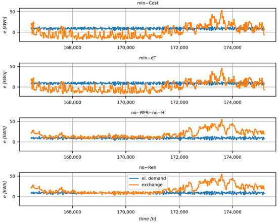
Figure 9.
Profiles of electricity demand and net electricity exchange in the 20th year for all four cases.
In the min-cost case (Figure 9), the electricity profile is significantly different since there is an export of electricity produced inside the microgrid, which reduces the net cost associated with the electricity exchange. For the min-dT case (Figure 9), the net exchange looks similar to the min-cost case but with a higher import-to-export ratio which increases the system cost. For the cases no-RES-no-H and no-Reh (Figure 9), electricity imports are substantial during the heating period. For the case no-Reh (Figure 9), the electricity demand is completely covered with imports. The simulation results show a drop in the average reservoir temperature over the 20 y period (Figure 10).
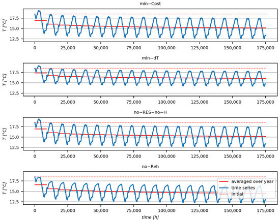
Figure 10.
The volume-averaged temperature of the reservoir over the 20-y simulation, with annually-averaged values.
Starting average temperature of the reservoir is 18.5 °C. The time series of the volume-averaged reservoir temperature show seasonal oscillations. The amplitude of annual oscillations is lower in the case where the heater is available for the use of freely available PV electricity. If results are compared over the 20-y simulation time, all cases show that the temperature drop is largest in the first year of the utilisation of reservoir heat and that temperature drop becomes steadier in the last 10 y of simulation. The largest 20-y span of average temperatures is between the cases min-dT and no-Reh—the first one having a temperature drop of 2.4 °C, and the other 4.0 °C. The drop in the temperature of the reservoir has, as a consequence, the drop in the heat pump performance since EST is lower than the case with reservoir reheating, and the heat pump uses more electricity for the same thermal load.
4.3. Techno-Economic Analysis Based on Long-Term Simulation Results
To demonstrate the runtime cost reduction resulting from the integration of renewables into the microgrid, analysis based on a 20-year time horizon is performed for two selected cases from Table 2. Technical analysis consists of energy flow analysis, and economic analysis is made based on a decomposition of costs in both scenarios. Decomposition of costs into CAPEX, OPEX and capital costs are compared in Figure 11.
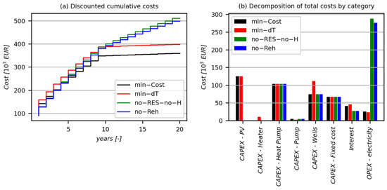
Figure 11.
Decomposition of costs. (a) represents discounted cumulative costs over a 20-year period; (b) represents the decomposition of undiscounted total costs by category.
Decomposition of costs shows that no-RES-no-H and no-Reh scenarios have lower CAPEX cost, as well as capital cost, while having higher OPEX costs. The dynamics of total payments, represented by cumulative discounted cost for the overall system (Figure 11a), shows that cases min-Cost and min-dT have low operating costs since they import less electricity from the DSO. On the other hand, these cases have higher capital costs for PV systems (Figure 11b). Case min-dT has the highest capital cost, but in the analysis of cumulative discounted payments, it stays below the no-Reh case during the whole simulation period. On the 20-year simulation results, the overall costs for the min-Cost case are 20% lower than no-RES-no-H cases, being the best and worst cases in this analysis. LCOE values are 65 EUR/MWh for the no-RES-no-H and 45 EUR/MWh for the min-Cost case. Table 3 summarises all the relevant results of the simulation.
Table 3.
Technical and economic outputs from the 20-year simulation.
The results for LCOE can be compared with the cost of electricity and gas for the alternative configuration having all electricity purchased from the DSO and heating from the gas boiler. If the latest retail prices in Croatia are taken into consideration, prices of electricity are at 130 EUR/MWh and gas at 38 EUR/MWh, as obtained from Eurostat [46], then the pondered overall LCOE for the import electricity-gas boiler alternative is 62 EUR/MWh for the import of the energy alone, i.e., without the cost of installation or escalation of prices. It has to be mentioned that Croatia has a reduced VAT for electricity and gas retail market is regulated, which keeps electricity and gas prices still subsidised
4.4. Mitigation of CO2 Emissions
After applying sufficient measures for reducing energy demands in the first place [47]—in combination with process intensification [48], the integration of renewable electricity from PV with geothermal heat pumps for heating and cooling is a good further step that mitigates the emissions of CO2 [49] acting as an alternative to 100% imported electricity and using boilers for heating.
According to Croatia’s energy bulletin [50], the specific CO2 emission factor from the electric grid, based on final consumption, is 106 gCO2/kWh. If we take into consideration all cases presented in this work (Table 4) and compare them to the alternative scenario with a total of 20-year emissions as 1270 tCO2, then all cases reduce at least 72% of the emissions, with the case min-dT reducing the emissions by 84%.
Table 4.
Estimated mitigation of CO2 emissions.
The cooling for the alternative scenario is assumed to be with the air-source heat pumps with the estimated COP equal to 3.5, and specific emissions from the burning of natural gas are approximately 220 gCO2/kWh-thermal. The efficiency of the natural gas boiler is estimated at a value of 95%.
4.5. Sensitivity Analysis Based on the Uncertainty of Input Costs
Sensitivity analysis is done for five parameters determining the costs: the price of electricity, investment cost for the most cost-intensive equipment being the HP, PV and cost of shallow geothermal wells (drilling and borehole heat exchanger, both expressed per meter of depth) and discount rate. The analysis is done for the +/−20% of the reference values and presented in Figure 12.
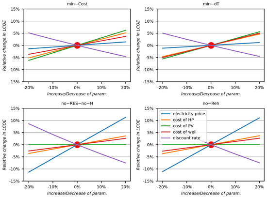
Figure 12.
Sensitivity analysis of cost with the variation in electricity price, cost of heat pump, cost of PV, cost of well and discount rate.
The most influential parameters for the min-Cost case is the cost of PV. The cost of PV has a negative influence on the LCOE, but this influence is less than 10% if the cost rises by +20%. For the min-dT case, the cost of PV and cost of a well are having a negative influence of the same value, which is also less than 10% if they rise to +20%. The cases no-RES-no-H and no-Reh are showing similar results since they are similar by structure. They both show high dependence on the price of electricity since the cost of electricity is the main contributor to OPEX cost. The increase in discount rate has a positive influence on LCOE, which is more visible in the no-RES-no-H and no-Reh cases since they generate more operating costs even after the loan has been settled in the first 10 y of operation. The break-even cost of electricity that would equate the LCOE’s of import electricity-gas boiler case and the min-Cost case at the value of 65 EUR/MWh would be approximately 23% higher than the current price and would stand at 160 EUR/MWh.
5. Conclusions
This paper presents the results of a long-term dynamic simulation of microgrid energy balance, including the heating and cooling system with a high share of renewable energy for the continental part of Croatia. A simulation was done with the model RES2GEO. Results show that the integration of renewable and intermittent energy sources like PV can be used for thermal recuperation of the shallow geothermal reservoir, resulting in the higher seasonal performance of the system and reducing the energy consumption of the heat pump. However, the case with the lowest thermal degradation of the reservoir is not the optimal solution from the economic point of view since it requires more geothermal wells, which increase the CAPEX and overall cost. The case with the lowest LCOE is the one that has a high share of renewable electricity from the PV. The use of own PV electricity in a microgrid that replaces the imported electricity is the most significant contributor to the low LCOE since it replaces the more expensive imported electricity. The use of a heater for thermal recuperation of the reservoir allows additional use of electricity and reduces the curtailment, even though it comes with a high capital cost of extra wells and heater. However, all cases are comparable with the alternative scenario in terms of LCOE. This means that all cases have LCOE lower than 62 EUR/MWh, which is the operating cost for natural gas heating and having electricity 100% imported from the DSO. Moreover, the installation of PV changes the net exchange profile, as seen from the DSO point of view. Results of the sensitivity analysis show that cases with the high import of electricity are very sensitive to prices of electricity, while the case with minimum cost is more sensitive to the price of the equipment, in this case, the PV.
Future work should include a Life Cycle Assessment for the use of PV in reheating the shallow geothermal reservoir. Future work should also include the analysis of mutual interference of geothermal wells since the subcooling of the reservoir with a larger number of wells can deteriorate the overall COP of the heating. Future work should also be focused on a more robust estimate of how to dimension the equipment, taking into account the uncertainty of the input data, like Sun insolation, outside temperature and consumption of electricity. In the end, since the use of equipment can be used for power-up and power-down regulation of the grid, the use of a microgrid as a demand response system towards the grid should be investigated. This role can significantly change the management system originally presented in this work.
Supplementary Materials
The following are available online at https://www.mdpi.com/article/10.3390/en14071923/s1: Algorithm for calculation of thermal demand.
Author Contributions
L.P.: Conceptualisation, Methodology, Investigation, Resources, Writing–original draft, Writing–review & editing, Supervision, Funding acquisition; D.L.: Investigation, Methodology; A.L.B.: Project administration, Writing–original draft; H.M.: Writing–review & editing; P.S.V.: Conceptualisation, Writing–review & editing, Supervision, Funding acquisition. All authors have read and agreed to the published version of the manuscript.
Funding
This research is done according to the project objectives of the project “Integration of shallow geothermal energy and variable renewables (RES2GEO)”, financed by the Ministry of science and education of the Republic of Croatia. This research has been supported by the EU project “Sustainable Process Integration Laboratory—SPIL”, project No. CZ.02.1.01/0.0/0.0/15_003/0000456 funded by EU “CZ Operational Programme Research, Development and Education”, Priority 1: Strengthening capacity for quality research.
Conflicts of Interest
The authors declare no conflict of interest.
Nomenclature
| A | area, m2 |
| C | total cost, EUR |
| c | specific heat capacity, J/kgK |
| d | discount rate, % |
| e | electric energy, kWh |
| H | height of calculation domain (reservoir), m |
| Inv | total investment, EUR |
| k | overall heat transfer coefficient, W/m2K |
| L | length, m |
| m | mass |
| N | number of years in analysis, - |
| p, P | price, EUR/kWh |
| q | thermal energy, kWh |
| r | radius, m |
| T | temperature, K or °C |
| t | time, h |
| V | volume, m3 |
| x | ratio, - |
| Subscripts | |
| B | boundary |
| cool | cooling |
| d | discounted |
| E, N, S, W | east, north, south and west orientation |
| el | electricity |
| Eq | equity |
| dem | demand |
| exp | exported |
| fix | fixed part of cost (not elsewhere specified) |
| H | heater |
| HP | heat pump |
| i | specific year |
| imp | imported |
| m2 | per sq. meter |
| net | netto |
| P | pump |
| R | reservoir |
| th | thermal |
| tot | total |
| w | water |
| Greek letters | |
| α | heat transfer coefficient, W/m2K |
| δ | distance, m |
| λ | thermal conductivity, W/mK |
| ρ | density, kg/m3 |
| ϕ | heat flux, W |
Abbreviations
| BHE | Borehole Heat Exchanger |
| CAPEX | Capital Expenditures |
| CHP | Combined Heat and Power |
| COP | Coefficient Of Performance (heat pump) |
| DSO | Distribution System Operator |
| EU | European Union |
| EUR | € (currency) |
| ELT | Entering Load Temperature (heat pump) |
| EST | Entering Source Temperature (heat pump) |
| GHG | Greenhouse Gas |
| GIS | Geographical Information Systems |
| GSHP | Ground Source Heat Pump |
| IPMT | Interest Payment |
| LCOE | Levelized Cost of Energy |
| LLT | Leaving Load Temperature (heat pump) |
| LST | Leaving Source Temperature (heat pump) |
| OPEX | Operating Expenses |
| PPMT | Principal Payment |
| PV | Photovoltaic |
| RES2GEO | Renewable Energy Sources to Geothermal |
| SG | Shallow Geothermal |
| TRT | Thermal Response Test |
References
- Klemeš, J.J. Assessing and Measuring Environmental Impact and Sustainability; Butterworth-Heinemann/Elsevier: Oxford, UK; Waltham, MA, USA, 2015; ISBN 978-0-12-799968-5. [Google Scholar]
- Perry, S.; Klemeš, J.; Bulatov, I. Integrating Waste and Renewable Energy to Reduce the Carbon Footprint of Locally Integrated Energy Sectors. Energy 2008, 33, 1489–1497. [Google Scholar] [CrossRef]
- Mohammad Rozali, N.E.; Wan Alwi, S.R.; Abdul Manan, Z.; Klemeš, J.J.; Hassan, M.Y. Optimal Sizing of Hybrid Power Systems Using Power Pinch Analysis. J. Clean. Prod. 2014, 71, 158–167. [Google Scholar] [CrossRef]
- EGEC Geothermal. Available online: https://www.egec.org/the-geothermal-energy-market-grows-exponentially-but-needs-the-right-market-conditions-to-thrive/ (accessed on 2 December 2020).
- Pérez, R.E. European Federation of Geologists. Available online: https://eurogeologists.eu/esteban-shallow-geothermal-energy-geological-energy-for-the-ecological-transition-and-its-inclusion-in-european-and-national-energy-policies/ (accessed on 1 December 2020).
- Dalla Longa, F.; Nogueira, L.P.; Limberger, J.; van Wees, J.-D.; van der Zwaan, B. Scenarios for geothermal energy deployment in Europe. Energy 2020, 206, 118060. [Google Scholar] [CrossRef]
- Kurevija, T. Analysis of potentials of shallow geothermal resources in heat pump systems in the city of Zagreb. Goriva Maz. 2008, 47, 373–390. [Google Scholar]
- Macenić, M.; Kurevija, T.; Strpić, K. Systematic review of research and utilisation of shallow geothermal energy in Croatia. Min. Geol. Pet. Eng. Bull. 2018, 33, 37–46. [Google Scholar] [CrossRef]
- Hajovsky, R.; Vojcinak, P.; Pies, M.; Koziorek, J. Thermal Response Test (TRT)—System for Measurement of Thermal Response of Rock Massif. IFAC Proc. Vol. 2013, 46, 126–131. [Google Scholar] [CrossRef]
- Bu, X.; Ran, Y.; Zhang, D. Experimental and Simulation Studies of Geothermal Single Well for Building Heating. Renew. Energy 2019, 143, 1902–1909. [Google Scholar] [CrossRef]
- He, Y.; Bu, X. A Novel Enhanced Deep Borehole Heat Exchanger for Building Heating. Appl. Therm. Eng. 2020, 178, 115643. [Google Scholar] [CrossRef]
- Rybach, L.; Mégel, T.; Eugster, W. At what time scale are geothermal resources renewable? In Proceedings of the World Geothermal Congress, Kyushu, Tohoku, Japan, 28 May–10 June 2000; Available online: https://www.geothermal-energy.org/pdf/IGAstandard/WGC/2000/R0900.PDF (accessed on 19 March 2021).
- Seyam, S.; Dincer, I.; Agelin-Chaab, M. Thermodynamic analysis of a hybrid energy system using geothermal and solar energy sources with thermal storage in a residential building. Energy Storage 2019. [Google Scholar] [CrossRef]
- The World Bank. Available online: https://data.worldbank.org/topic/urban-development (accessed on 1 December 2020).
- European Commission. 2030 Climate & Energy Framework. Available online: https://ec.europa.eu/clima/policies/strategies/2030_en (accessed on 1 December 2020).
- Kerry, S.; Baume, O.; Caruso, G.; Ulrich, L. GIS-based modelling of shallow geothermal energy potential for CO2. Renew. Energy 2016, 86, 1023–1036. [Google Scholar] [CrossRef]
- Walch, A.; Mohajeri, N.; Gudmundsson, A.; Scartezzini, J.-L. Quantifying the Technical Geothermal Potential from Shallow Borehole Heat Exchangers at Regional Scale. Renew. Energy 2021, 165, 369–380. [Google Scholar] [CrossRef]
- Ramos-Escudero, A.; García-Cascales, M.S.; Cuevas, J.M.; Sanner, B.; Urchueguía, J.F. Spatial Analysis of Indicators Affecting the Exploitation of Shallow Geothermal Energy at European Scale. Renew. Energy 2021, 167, 266–281. [Google Scholar] [CrossRef]
- Perković, L.; Mikulčić, H.; Pavlinek, L.; Wang, X.; Vujanović, M.; Tan, H.; Baleta, J.; Duić, N. Coupling of cleaner production with a day-ahead electricity market: A hypothetical case study. J. Clean. Prod. 2017, 143, 1011–1020. [Google Scholar] [CrossRef]
- Urbaniec, K.; Mikulčić, H.; Duić, N. SDEWES 2014—Sustainable Development of Energy, Water and Environment Systems. J. Clean. Prod. 2016, 130, 1–11. [Google Scholar] [CrossRef]
- Perković, L.; Mikulčić, H.; Duić, N. Multi-objective optimisation of a simplified factory model acting as a prosumer on the electricity market. J. Clean. Prod. 2018, 167, 1438–1449. [Google Scholar] [CrossRef]
- Mikulčić, H.; Ridjan Skov, I.; Dominković, D.F.; Wan Alwi, S.R.; Manan, Z.A.; Tan, R.; Duić, N.; Hidayah Mohamad, S.N.; Wang, X. Flexible Carbon Capture and Utilisation technologies in future energy systems and the utilisation pathways of captured CO2. Renew. Sustain. Energy Rev. 2019, 114, 109338. [Google Scholar] [CrossRef]
- Wood, E. Microgrid Knowledge. Available online: https://microgridknowledge.com/microgrid-defined/ (accessed on 1 December 2020).
- Ali, A.; Li, W.; Hussain, R.; He, X.; Williams, B.W.; Memon, A.H. Overview of Current Microgrid Policies, Incentives and Barriers in the European Union, United States and China. Sustainability 2017, 9, 1146. [Google Scholar] [CrossRef]
- Al-Khoury, R. Computational Modeling of Shallow Geothermal Systems; CRC Press: Boca Raton, FL, USA, 2012; ISBN 978-0-429-16576-4. [Google Scholar]
- Vieira, A.; Alberdi-Pagola, M.; Christodoulides, P.; Javed, S.; Loveridge, F.; Nguyen, F.; Cecinato, F.; Maranha, J.; Florides, G.; Prodan, I.; et al. Characterisation of Ground Thermal and Thermo-Mechanical Behaviour for Shallow Geothermal Energy Applications. Energies 2017, 10, 2044. [Google Scholar] [CrossRef]
- Casasso, A.; Sethi, R.G. POT: A Quantitative Method for the Assessment and Mapping of the Shallow Geothermal Potential. Energy 2016, 106, 765–773. [Google Scholar] [CrossRef]
- Ondreka, J.; Rüsgen, M.I.; Stober, I.; Czurda, K. GIS-Supported Mapping of Shallow Geothermal Potential of Representative Areas in South-Western Germany—Possibilities and Limitations. Renew. Energy 2007, 32, 2186–2200. [Google Scholar] [CrossRef]
- Tissen, C.; Menberg, K.; Benz, S.A.; Bayer, P.; Steiner, C.; Götzl, G.; Blum, P. Identifying Key Locations for Shallow Geothermal Use in Vienna. Renew. Energy 2020, 167, 1–19. [Google Scholar] [CrossRef]
- Dalla Santa, G.; Galgaro, A.; Sassi, R.; Cultrera, M.; Scotton, P.; Mueller, J.; Bertermann, D.; Mendrinos, D.; Pasquali, R.; Perego, R.; et al. An Updated Ground Thermal Properties Database for GSHP Applications. Geothermics 2020, 85, 101758. [Google Scholar] [CrossRef]
- Somogyi, V.; Sebestyén, V.; Nagy, G. Scientific Achievements and Regulation of Shallow Geothermal Systems in Six European Countries—A Review. Renew. Sustain. Energy Rev. 2017, 68, 934–952. [Google Scholar] [CrossRef]
- Cai, S.; Li, X.; Zhang, M.; Fallon, J.; Li, K.; Cui, T. An Analytical Full-Scale Model to Predict Thermal Response in Boreholes with Groundwater Advection. Appl. Therm. Eng. 2020, 168, 114828. [Google Scholar] [CrossRef]
- Meng, B.; Vienken, T.; Kolditz, O.; Shao, H. Evaluating the Thermal Impacts and Sustainability of Intensive Shallow Geothermal Utilisation on a Neighborhood Scale: Lessons Learned from a Case Study. Energy Convers. Manag. 2019, 199, 111913. [Google Scholar] [CrossRef]
- Vienken, T.; Kreck, M.; Dietrich, P. Monitoring the Impact of Intensive Shallow Geothermal Energy Use on Groundwater Temperatures in a Residential Neighborhood. Geotherm. Energy 2019, 7, 8. [Google Scholar] [CrossRef]
- Lyu, W.; Li, X.; Yan, S.; Jiang, S. Utilizing Shallow Geothermal Energy to Develop an Energy Efficient HVAC System. Renew. Energy 2020, 147, 672–682. [Google Scholar] [CrossRef]
- Sofyan, S.E.; Hu, E.; Kotousov, A.; Riayatsyah, T.M.I.; Thaib, R. Mathematical Modelling and Operational Analysis of Combined Vertical–Horizontal Heat Exchanger for Shallow Geothermal Energy Application in Cooling Mode. Energies 2020, 13, 6598. [Google Scholar] [CrossRef]
- Kurevija, T.; Macenić, M.; Borović, S. Impact of Grout Thermal Conductivity on the Long-Term Efficiency of the Ground-Source Heat Pump System. Sustain. Cities Soc. 2017, 31, 1–11. [Google Scholar] [CrossRef]
- Sikos, L.; Klemeš, J. Reliability, Availability and Maintenance Optimisation of Heat Exchanger Networks. Appl. Therm. Eng. 2010, 30, 63–69. [Google Scholar] [CrossRef]
- Choi, H.; Kim, J.; Shim, B.O.; Kim, D. Characterization of Aquifer Hydrochemistry from the Operation of a Shallow Geothermal System. Water 2020, 12, 1377. [Google Scholar] [CrossRef]
- Kljajić, M.V.; Anđelković, A.S.; Hasik, V.; Munćan, V.M.; Bilec, M. Shallow Geothermal Energy Integration in District Heating System: An Example from Serbia. Renew. Energy 2020, 147, 2791–2800. [Google Scholar] [CrossRef]
- Fan, Y.V.; Varbanov, P.S.; Klemeš, J.J.; Romanenko, S.V. Urban and Industrial Symbiosis for Circular Economy: Total EcoSite Integration. J. Environ. Manag. 2021, 279, 111829. [Google Scholar] [CrossRef]
- Python Software Foundation. Python Language Reference, Version 3.8. Available online: www.python.org (accessed on 10 February 2021).
- ECOFOREST Heat Pumps Technical Data. Available online: www.ecoforest.es (accessed on 1 December 2020).
- Connolly, D.; Drysdale, D.; Hansen, K.; Novosel, T. Creating Hourly Profiles to Model both Demand and Supply. Background Report 2, Stratego Project. Available online: https://heatroadmap.eu/wp-content/uploads/2018/09/STRATEGO-WP2-Background-Report-2-Hourly-Distributions-1.pdf (accessed on 19 March 2021).
- Photovoltaic Geographical Information System. Available online: Ec.europa.eu/jrc/en/pvgis (accessed on 10 March 2021).
- Eurostat. Available online: https://ec.europa.eu/eurostat. (accessed on 1 December 2020).
- Chew, K.H.; Klemeš, J.J.; Wan Alwi, S.R.; Manan, Z.A. Process Modifications to Maximise Energy Savings in Total Site Heat Integration. Appl. Therm. Eng. 2015, 78, 731–739. [Google Scholar] [CrossRef]
- Klemeš, J.J.; Varbanov, P.S. Process Intensification and Integration: An Assessment. Clean Technol. Environ. Policy 2013, 15, 417–422. [Google Scholar] [CrossRef]
- Baleta, J.; Mikulčić, H.; Klemeš, J.J.; Urbaniec, K.; Duić, N. Integration of Energy, Water and Environmental Systems for a Sustainable Development. J. Clean. Prod. 2019, 215, 1424–1436. [Google Scholar] [CrossRef]
- Ministry of Environment and Energy of the Republic of Croatia, Annual Energy Report—Energy in Croatia. 2018. Available online: www.eihp.hr/wp-content/uploads/2020/04/Energija2018.pdf (accessed on 11 March 2021).
Publisher’s Note: MDPI stays neutral with regard to jurisdictional claims in published maps and institutional affiliations. |
© 2021 by the authors. Licensee MDPI, Basel, Switzerland. This article is an open access article distributed under the terms and conditions of the Creative Commons Attribution (CC BY) license (https://creativecommons.org/licenses/by/4.0/).