Article

Numerical Study of Vibration Characteristics for Sensor Membrane in Transformer Oil

1
State Grid Shanghai Electrical Power Research Institute, Shanghai 200437, China
2
MOE Key Laboratory of Micro/Nano Systems for Aerospace, Northwestern Polytechnical University, Xi’an 710072, China
3
MOE Key Laboratory of Thermo-Fluid Science and Engineering, Xi’an Jiaotong University, Xi’an 710049, China
*
Author to whom correspondence should be addressed.
Energies 2021, 14(6), 1662; https://doi.org/10.3390/en14061662
Submission received: 23 February 2021 / Revised: 11 March 2021 / Accepted: 15 March 2021 / Published: 17 March 2021

Abstract

:
Membrane is the most important element of extrinsic Fabry-Perot interferometer sensors. Studying the relationship between working medium viscosity and membrane vibration characteristics are critical to the sensor design because the transformer oil viscosity will cause viscous loss during membrane vibration. The numerical investigation of membrane vibration characteristics in transformer oil is performed based on the finite element method. Besides, the effect of energy loss caused by viscosity is examined. It is firstly showed that the membrane has the highest sensitivity for the first-order vibration mode, and the transformer oil reduces the fundamental frequency by 60%. Subsequently, when viscosity and heat loss are considered, the amplitude is less than one-fifth of that without energy loss. The viscosity has a more significant effect on the velocity and temperature fields when the vibration frequency is close to the natural frequency. Finally, viscosity has a remarkable impact on the time domain response. Mechanical energy is converted into thermal energy during the vibration and the amplitude will gradually decrease with time. The effect of energy loss caused by viscosity on the membrane vibration characteristics is revealed, which would be important for an oil-immersed membrane design.

1. Introduction

Transformers play an important role in power transmission systems. Partial discharge inside the transformer may cause insulation failure, and even catastrophic accidents in severe cases [1]. The detection of partial discharge is widely used in insulation diagnosis for electrical equipment. The insulation failure can be found immediately by monitoring the evolution of discharge process, and the online detection can act as a preventive role before failure occurs [2].
Ultrasonic detection method has become one of the most important methods for online partial discharge detection because it can effectively resist electromagnetic interference in transformers [3]. Nowadays, piezoelectric ceramic sensor is the most popular external ultrasonic sensor [4]. Although the external sensor is convenient to install, it is sensitive to the influence of the external environment. Besides, ultrasonic waves that were generated by partial discharge will be attenuated when they transmit through transformer oil or a transformer oil tank wall, and multipath transmission will cause positioning difficulties. These shortcomings would greatly hinder the application of external sensors [5]. As for the built-in sensor, it has many advantages, such as no chemical reaction with insulating medium, good insulation, stable operation and small size, etc. [6] Recently, the extrinsic Fabry-Perot interferometer (EFPI) sensor has become one of the most popular built-in sensors due to its advantages, such as anti-electromagnetic interference, small size, easy signal processing, flexible application and operation in extreme environments [7]. It is found that, the Fabry-Perot membrane has a remarkable effect on both the amplitude-frequency characteristics and sensitivity of the sensor.
At present, there are many pieces of research on the design of sensor membranes. For example, Jiang et al. [8] developed highly sensitive sensor membranes by changing the membrane radius and thickness. In their study, in order to avoid a signal interference caused by magnetic vibration of internal winding in the transformer and noise generated by the cooling oil circulation, the membranes natural frequency was controlled within an appropriate range. A cantilever beam sensor membrane was designed by Su et al. [9], and the effect of thermal stress on the natural frequency, sensitivity and stability for the membrane was analyzed. Ghildiyal et al. [10] manufactured a metal membrane with a measurement range of 0–100 mbar by stretching membrane and changing stress. Liu et al. [11] developed a high sensitivity membrane by etching permanent ripples on the membrane. The mechanical property of this membrane would change as the ripple depth changes. Yu and Zhou [12] used a controlled thermal bonding technique to process EFPI sensors that can work at 300 ℃, which further increases the application range of the EFPI sensors. Bo et al. [13] used polyethylene oxide (a strongly hydrophilic material) to fabricate sensors for detecting humidity variations. Liao et al. [14] used polyethylene terephthalate as the membrane material and it was applied to highly sensitive acoustic detection. Liu et al. [15] deposited a perylene diimide derivative as a sensitive film on the membrane, and developed a new type of optical fiber sensor with a temperature sensitivity of 9.8 pm/℃ by using the change in the refractive index of the membrane under hydrazine vapor. Kendir and Yaltkaya [16] used magnetostrictive material as the sensor membrane and successfully fabricated fiber optic magnetic field sensors that can sense changes in the magnetic field. Li et al. [17] demonstrated through experiments a low-cost fiber optic accelerometer based on a polyethylene membrane, and the measured sensitivity was 135 mV/g, which greatly reduced the production cost of the probe.
The above references mainly optimize the performance of the sensor membrane from the aspects of the shape of the membrane, manufacturing materials, processing technology, and application scenarios. However, when the sensor is arranged in the transformer, the membrane is surrounded by transformer oil, and the oil around the membrane will affect the vibration characteristics, causing the design deviations from the actual application. Some scholars have performed related researches on the relationship between membrane vibration and surrounding medium. Kilic et al. [18] analyzed the influence of static pressure fluctuation on the vibration performance of the sensor membrane. The results show that the influence of static pressure fluctuation could be ignored when the cavity was interconnected with the transformer oil. Lesieutre [19] conducted a corresponding study on the influence of load on structural modal damping and found that an increase in tensile load will increase the natural frequency, but reduce the modal damping. Minami [20] studied the vibration of the membrane structure in the air environment. Under the assumption that air is an incompressible fluid, the additional mass of air is derived as a coefficient related to the air density and the shape of the membrane. Sygulski [21] used the boundary element method to establish the discrete dynamic equation of the free vibration of the membrane structure in the air environment, and numerically analyzed the influence of air on the membrane vibration. Henn et al. [22] simulated the fluid dynamics of transient fluid-structure interaction, and the results showed that there is a clear flow velocity in a narrow area close to the membrane surface, and the additional mass layer has no clear boundary. These studies have analyzed the influence of air on the vibration characteristics when the membrane is vibrating in the air. However, in these applications, the effect of viscosity during the vibration process is negligible and does not reveal the effect of viscous damping on the vibration characteristics. In working media with non-negligible viscosity (such as transformer oil), viscosity will cause viscosity loss and heat loss, thereby affecting vibration characteristics. Changes in vibration characteristics will cause the sensor’s signal reception deviations from the design target.
Therefore, in the present paper, the EFPI membrane vibration performance in transformer oil was numerically studied, and a membrane vibration model that couples thermal viscosity and flow heat transfer was established. The effects of viscous damping and mass damping on the natural frequency, sensitivity, amplitude-frequency characteristics and time domain response of the membrane were analyzed. This study is meaningful for understanding the influence of transformer oil on membrane vibration and the design of membranes arranged in transformer oil.

2. Physical Model and Computational Method

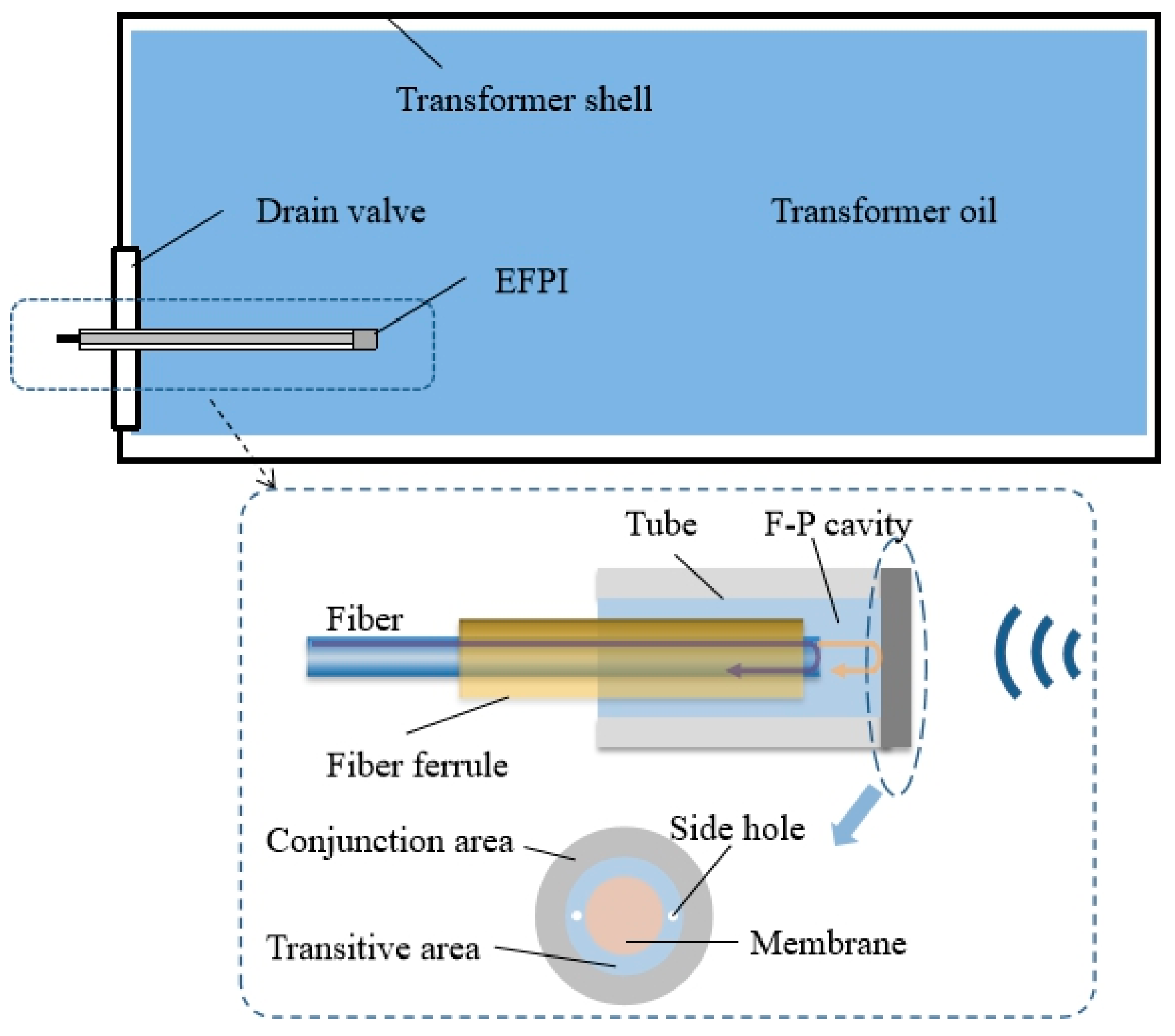
2.1. Physical Model and Geometric Parameters

The scheme for an EFPI sensor and its location in a transformer oil tank is presented in Figure 1. The sensor is located in the transformer drain valve, and the sensor is surrounded by transformer oil.
In the present study, the EFPI sensor is used for partial discharge detection in an oil-immersed transformer. In order to eliminate the impact of static pressure fluctuation, the EFPI sensor cavity is interconnected with the transformer oil, so that the internal pressure and external pressure of the sensor should be the same [23]. The EFPI sensor is composed of membrane, optical fiber and cavity. Light is transmitted through optical fiber. Part of the light is reflected on the end face of the fiber and the rest of the light is reflected at the membrane. The ultrasonic waves generated by the partial discharge will cause the vibration of membrane, then the resonant cavity length will changes and lead to change of output light intensity. By demodulating the output light intensity, the discharge situation can be obtained. The correlation between the output light intensity and cavity length is presented in Equation (1) [24].
I ( λ , l ) = I 0 ( λ ) R 1 + R 2 2 R 1 R 2 cos ( 4 π l / λ ) 1 + R 1 R 2 2 R 1 R 2 cos ( 4 π l / λ )
where I0 (λ) is the input light intensity; I (λ, l) is the output light intensity; λ is the incident light wavelength; l is the cavity length; R1 is the fiber end face reflectivity; R2 is the membrane reflectivity. When R1 = 0.4, R2 = 0.4, λ = 1550 nm and I0 (λ) = 1 cd, the variations of output light intensity with cavity length is presented in Figure 2.
As shown in Figure 2, when the cavity length changes with λ/2, the output light intensity changes with a single period [25]. When the change of cavity length is less than λ/4, the quadrature phase point (Q point) can be set as an initial operating point and static operating point, and then the output light intensity would change almost linearly with the cavity length at this time. In this linear region, the sensor has high sensitivity and responds fast, and it is suitable for ultrasonic and vibration signal detections [26].
Based on the principle of elasticity, when the deformation is less than 25% of membrane thickness, it can be considered that the membrane deformation has a linear relationship with the pressure [27]. The scheme for a circular membrane deformation under uniform pressure is presented in Figure 3.
It shows that the largest deformation is at the membrane center, which can be formulated with Equation (2) [28].
Y max = 3 ( 1 μ 2 ) p 16 E h 3 a 4
where h is the thickness; a is the radius of the membrane; E is the Young’ s modulus; μ is the Poisson’s ratio; Ymax is the largest deformation; p is the pressure. The responsive sensitivity of the membrane can be formulated with Equation (3). It shows that the sensitivity (S) is proportional to the square of membrane radius and inversely proportional to the cube of the membrane thickness. Therefore, the membrane sensitivity can be improved by increasing the membrane radius or decreasing the membrane thickness.
S = Y max p = 3 ( 1 μ 2 ) 16 E h 3 a 4
The spectrum of acoustic signals generated by partial discharges is usually from 10 kHz to 300 kHz. The environmental noise frequency and magnetic vibration frequency of the internal winding in the transfer are usually below 60 kHz [3]. Therefore, the detection frequency of ultrasonic sensors is usually setting from 60 kHz to 300 kHz. The natural frequency of a free vibrating circular membrane is formulated in Equation (4) [29]:
f = ω / 2 π = c 0 4 π E 3 ρ M ( 1 μ 2 ) ( h a 2 )
where ω is the angular frequency; c0 is the model coefficient; ρM is the membrane density. From Equation (4), it shows that the natural frequency of the membrane is proportional to the membrane thickness and inversely proportional to the square of the free membrane radius, which means, as the membrane sensitivity (S) increases, the natural frequency (f) of the membrane decreases. Therefore, when designing a sensor membrane, both the sensitivity and natural frequency should be considered at the same time.
In the present study, due to the requirements for natural frequency and sensitivity in partial discharge detection, the membrane radius (a) is set to 0.6 mm and the thickness (h) is set to 40 μm. As shown in Figure 4, the membrane is surrounded by transformer oil. The membrane is fixed at the periphery and is free to vibrate along the direction normal to membrane surface.
The membrane is made of quartz, and its mechanical properties are presented in Table 1 [30]. Furthermore, for the present simulations, the diameter for the thermoviscous acoustic domain (d1) is set to 0.8 mm, and the diameter for the pressure acoustic domain (d2) is set to 1.1 mm. The thermal properties for transformer oil are presented in Table 2 [30], which shows that the thermal properties of transformer oil should vary with temperature.
ρ = 1055.05 0.581753 T 6.40532 10 5 T 2     ( 223   K T 373   K )
η = { 4492.202 64.74088 T + 0.349900959 T 2 8.40477 10 4 T 3 + 7.57041667 10 7 T 4     ( 243   K T 293   K ) 91.4525 1.33227058 T + 0.0077768 T 2 2.272714 10 5 T 3 + 3.324197 10 8 T 4 1.94631 10 11 T 5     ( 293   K T 373   K )
c p = { 117,056.38 + 1816.762 T 10.305786 T 2 + 0.02566919 T 3 2.36742424 10 5 T 4     ( 223   K T 293   K ) 13,408.1491 + 123.044152 T 0.335401786 T 2 + 3.125 10 4 T 3     ( 293   K T 373   K )
k = 0.134299084 8.04973822 10 5 T     ( 223   K T 373   K )

2.2. Governing Equations and Computational Methods

In the existing research, the relevant membrane vibration model considering viscous loss and heat loss has not been established, while the heat loss and viscous loss are inevitable during the vibration process. In order to simplify the calculation of membrane vibration in transformer oil, the model adopted in the present paper is based on the following assumptions: (1) ignore the influence of transformer oil main flow velocity on membrane vibration; (2) the ambient temperature is constant; (3) ignore the influence of the thermal expansion of the membrane on the vibration characteristics; (4) it is considered that the conditions on both sides of the membrane are exactly the same, and the influence of the space restriction of the Fabry-Perot cavity is not considered. The specific steps of the numerical study of the effect of transformer oil viscosity on vibration characteristics are shown in Figure 5.
The membrane would vibrate under the effect of ultrasound, and the mass damping and viscous damping will appear due to the existence of transformer oil attached to the membrane surface and affect the membrane vibrations. The fluid-solid coupled vibration equations for the membrane are presented as follows [31]:
M s w ¨ ( t ) + C s w ˙ ( t ) + K s w ( t ) = F T ( t ) + F P ( t , w ( t ) , w ˙ ( t ) , w ¨ ( t ) )
where Ms is mass matrix; Cs is damping matrix; Ks is stiffness matrix; FT is external load; Fp is the force generated by the structure vibration; w ¨ ( t ) , w ˙ ( t ) and w ( t ) are the acceleration, velocity and displacement of membrane vibration at moment t, respectively.
When sound propagates in small geometric structures, viscous loss occurs near the solid wall. The acoustic-thermal effect would be the most obvious when the membrane is in resonance, which would reduce the natural vibration frequency of the membrane. In order to take the acoustic-thermal effect into account, the viscous loss and heat transfer should be added to the governing equations for the present simulations. The specific governing equation is as follows [32]:
Continuity equation:
i ω ρ = ρ 0 ( v )
where ρ is the background density; ρ0 is the average density; ω is angular frequency; i is the imaginary number; v is the velocity vector.
Momentum equations:
{ ρ [ v t + ( v ) v ] = p + η 2 v + ( η B + 4 3 η ) ( v ) η = b 0 ( 1 Y + 0.8 + 0.761 Y ) η B = 1.002 b 0 Y
where η is shear viscosity; ηB is bulk viscosity; p is pressure; b0 is second virial coefficient; Y is the relative collision frequency.
Energy equations:
i ω ( ρ 0 c p T T 0 α 0 p ) = ( k T )
where cp is constant pressure heat capacity; k is thermal conductivity; α0 is thermal expansion coefficient; T is temperature; T0 is average temperature.
The boundary condition of the membrane is the fixed boundary, that is to say, the boundary of the membrane will restrain the vibration, which are as follows:
w | r = a = 0 & w r | r = a = 0
where w is the displacement; a is the radius of membrane.
The interface between the membrane and transformer oil is set as the fluid-solid coupling boundary. At this interface, the velocity of the fluid domain is equal to the velocity of the solid domain, and no cavitation area occurs, which is formulated as follows:
v ( t ) fluid = v ( t ) solid
where v ( t ) fluid is the velocity of the transformer oil; v ( t ) solid is the vibration velocity of the membrane.
The interface of thermoviscous acoustic domain and pressure acoustic domain is set as the adiabatic boundary, where the heat loss and viscosity loss have no effect outside this interface. It is formulated as follows:
k T = 0
The outer boundary of pressure acoustic domain is set as the acoustic radiation boundary [33], which means when wave is transmitted at this boundary, it will be completely absorbed. It is formulated as follows:
( 1 ρ p ) + ( i ω 2 c 2 + 2 d 2 ) p 2 ρ = 0
where ω is angular frequency; c is the speed of sound transmission; d2 is the pressure acoustic domain.
In the present study, the above equations are solved with the commercial software COMSOL Multiphysics 5.2 (COMSOL AB, Stockholm, Sweden). When all residuals of the calculations are less than 10−6, the computational results are considered to be convergence.

3. Model Validation and Grid Independence Test

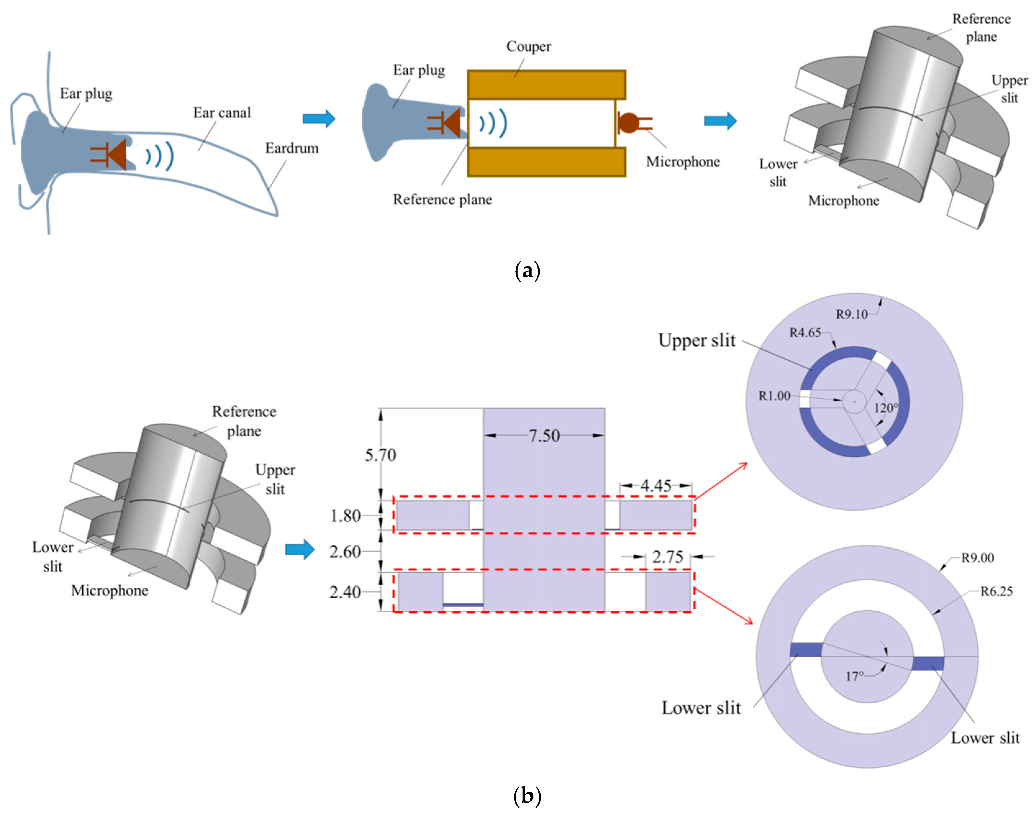
3.1. Model Validations

In the present paper, the occluded-ear canal simulator with the international standard IEC 60318-4 [34] is adopted for the validation of the thermoviscous acoustic computational model. The occluded-ear canal simulator is a device used to simulate the acoustic characteristics between the headphones and the eardrum. This simulator is often used to test headphones or hearing aids coupled to the eardrum. The working principle for the occluded-ear canal simulator is presented in Figure 6a.
It shows that the human ear model is composed of eardrum, earplug and ear canal. In order to imitate the working process of human ear, the simulator is required to simulate both the acoustic energy loss at the eardrum and the acoustic characteristics of ear canal. The simulator is simplified to a cylindrical channel with two additional ring channels, where the central cylindrical channel and additional ring channel are connected by slits [34]. The central cylindrical channel represents the human ear canal. The lower end surface of the cylindrical channel is set as the measuring microphone, which represents the eardrum of the human ear. The pressure on the lower end surface of the cylindrical channel represents the pressure of the human ear. The upper end surface of the cylindrical channel is the sound inlet reference plane, which represents the sound entrance. The sound leakage between the eardrum and the ear canal is produced in the upper slits, and the sound energy loss at the eardrum is produced in the lower slits. The geometric model for the occluded-ear canal simulator is presented in Figure 6b. The entrance diameter of the central cylindrical channel is 7.5 mm and its length is 12.5 mm. The upper slits are composed of three equally spaced sectors with a central angle of 120°, and the slits height is 69 μm. The lower slits are symmetrically distributed, and the slits height is 170 μm.
The slit area of the simulator is set as thermoviscous acoustic domain, and the thermoviscous loss in the slits is the main reason for acoustic energy loss. The rest of the simulator is set as a pressure acoustic domain, and the simulator channel is filled with air (296.13 K). The inlet reference plane of the simulator is set as a vibration boundary with an amplitude of 5 μm and a frequency range of 100 Hz–10,000 Hz. The microphone plane is set as the series resonant circuit (RLC) impedance boundary and the rest of the boundaries are set as sound hard boundaries [35].
The transfer impedance is often adopted to reflect the hindering effect on sound transmission for the human ear, and the transfer impedance (Ztrans) is defined as follows [34]:
Z trans = p mic Q in
where pmic is the average pressure at the eardrum; Qin is the air volume flow rate at the inlet reference plane, which is mainly depended on the displacement and the frequency of the inlet plane. When the inlet volume flow rate is kept constant, the sound pressure at the microphone is dependent on the transfer impedance between the inlet reference plane and the microphone.
The standard values and tolerances of transfer impedance for occluded-ear canal simulator with different frequencies are listed in Table 3 [34]. It shows that, when the frequency changes from 100 Hz to 10,000 Hz, the standard value tolerances of transfer impedance for the simulator would change from 1.56% to 9.52%. The variations of transfer impedance for occluded-ear canal simulator with frequency are presented in Figure 7. It shows that the present results based on the thermoviscous acoustic model can agree with the IEC60318-4 standard values, where the maximum deviation is 4.28%, and the average deviation is 1.41%.

3.2. Grid Independence Test

The computational grid is presented in Figure 8. In the present study, the unstructured grid was constructed for the simulations. The grids are intensified near the interface between solid and fluid regions. The computational domain is divided into membrane area (Zone 1), thermoviscous acoustic area (Zone 2) and pressure acoustic area (Zone 3).
In the present work, seven sets of grids were constructed for the test. The computational results for natural frequency (f), maximum temperature difference (ΔT) and maximum pressure drop (Δp) with different grids are presented in Table 4. It shows that the grid with total element number of 107,804 (Grid 5) should be good enough for the test. As for Grid 5, the minimum grid element size is 0.003 mm and the maximum grid element size is 0.03 mm for Zone 1. The minimum grid element size is 0.008 mm and the maximum grid element size is 0.08 mm for Zone 2. The minimum grid element size is 0.01 mm and the maximum grid element size is 0.15 mm for Zone 3. The deviations of natural frequency (f), maximum temperature difference (ΔT) and maximum pressure drop (Δp) between grids with a total element number of 107,804 (Grid 5) and 153,615 (Grid 6) is less than 2%. Therefore, similar grid settings to the test grid with a total grid number of 107,804 (Grid 5) were adopted for the following simulations.

4. Results and Discussion

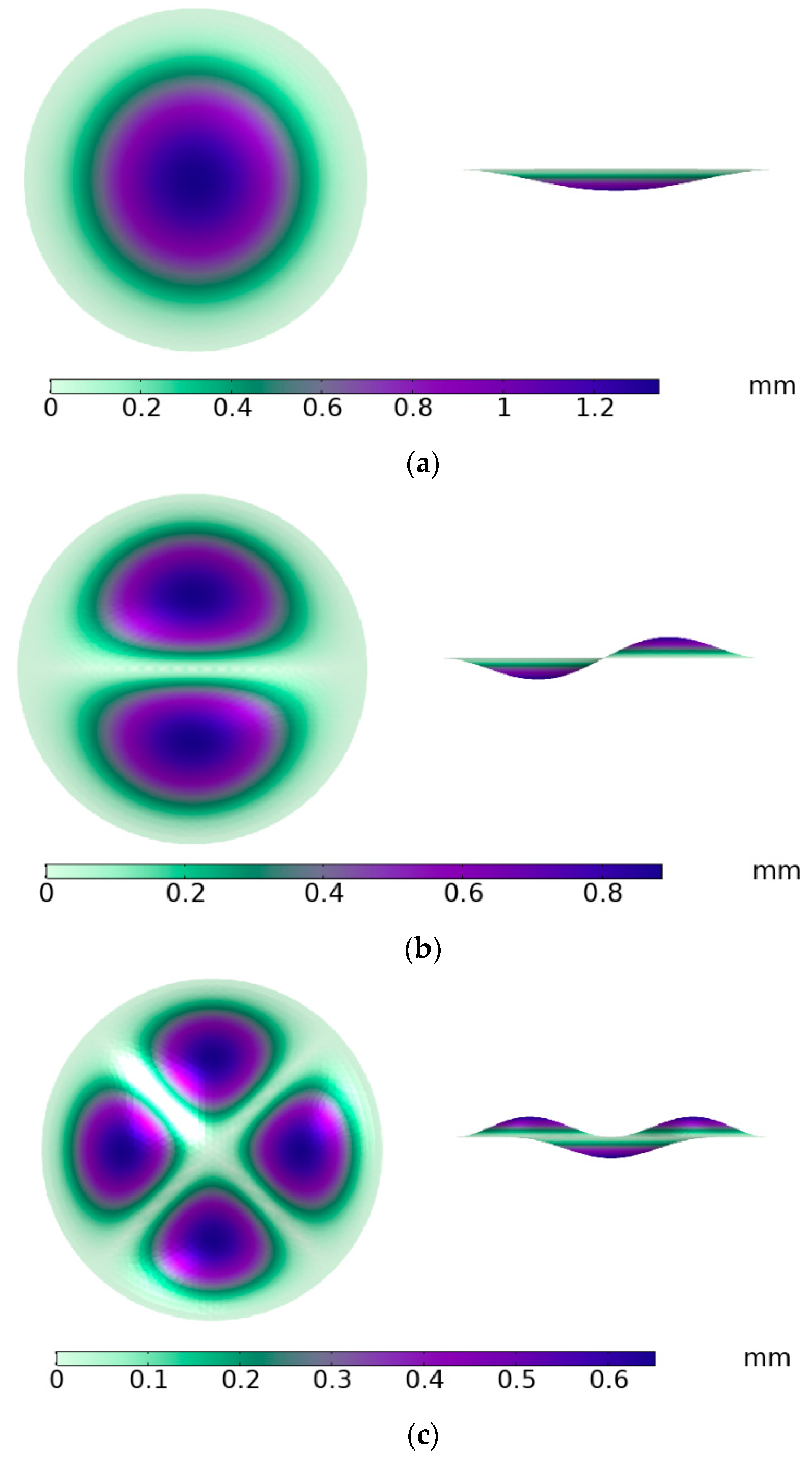
4.1. Natural Frequency Analysis

In the present study, the natural frequency of the EFPI membrane is analyzed for different conditions. Firstly, the membrane is assumed to vibrate freely without the effect of transfer oil. Then, the membrane is assumed to vibrate in the transfer oil with or without the effect of oil viscosity. The vibration modes for membrane under free vibration condition without transfer oil are presented in Figure 9. It shows that, for the first-order vibration mode, the membrane has the same phase point. As with the higher order vibration modes, the membrane phase point is different, which should be harmful for ultrasonic signal demodulation. This means, for the higher vibration mode, it is difficult to predict the vibration of membrane through the intensity of output light. Therefore, for the design of the membrane, the first-order natural frequency of the membrane should be controlled within the ultrasonic signal detection range, while the higher order natural frequency of the membrane should exceed the maximum value of the partial discharge ultrasonic signal frequency. In addition, it is also found that, as the membrane vibration mode order increases, the membrane vibration amplitude decreases gradually, which indicates that the membrane sensitivity should be the highest for the first-order vibration mode.
The natural frequency of membranes under different vibration conditions are presented in Table 5. It shows that, as compared with the free vibration model, when the membrane vibrates in the non-viscous transformer oil, its first-order natural frequency decreases by 61.1%, its second-order natural frequency decreases by 51.7%, and third-order natural frequency decreases by 46.1%, respectively; when the membrane vibrates in the viscous transformer oil, its first-order natural frequency decreases by 61.3%, the second-order natural frequency decreases by 52%, and third-order natural frequency decreases by 46.4%, respectively. This indicates that the effect of transformer oil on the natural frequency of membrane vibration is remarkable, especially for the lower-order vibration modes. As compared with free vibration model, when the membrane vibrates in the transformer oil, the mass damping effect should increase and the natural frequency of membrane decrease. Furthermore, when the membrane works in viscous transformer oil, the oil density and oil mass distribution would be changed due to the temperature variations of the oil surrounding the membrane surface, and then the natural frequency of the membrane will also be affected. However, since the temperature variation of oil surrounding the membrane surface is relatively small, its effect on the natural frequency of the membrane would be ignored.

4.2. Amplitude-Frequency Characteristics

The pressure of ultrasonic sound generated by the partial discharge can reach 0–1000 Pa [8]. In the present study, the membrane surface load is assumed to be 100 Pa, and the amplitude-frequency characteristics were analyzed for the membrane vibration under different conditions. Firstly, the variations of viscous transformer oil velocity around the membrane under first-order vibration mode are analyzed. The velocity distributions for viscous transformer oil are presented in Figure 10.
It shows that, as the membrane vibrates, the oil velocity gradient near the surface of the membrane is relatively large, which will lead to viscous loss for membrane vibration. It can also be found that, when the vibration frequency of the membrane is close to its natural frequency (f = 122,460 Hz, Figure 11), the vibration amplitude of the membrane is larger, and the effect on the oil velocity field caused by vibrations are wider and more significant. Otherwise, when the vibration frequency of the membrane is not close to its natural frequency (f = 122,460 Hz, Figure 11), the effect on the oil velocity field caused by the vibration is relatively small. The variation of maximum velocity for viscous transformer oil around the membrane with a vibration frequency is presented in Figure 11. It is shows that, when the vibration frequency of membrane approaching its natural frequency (f = 122,460 Hz), the oil velocity around the membrane increases. Otherwise, the oil velocity around the membrane decreases. As the vibration frequency of the membrane equals its natural frequency (f = 122,460 Hz), the oil velocity around the membrane reaches its highest.
The temperature distributions for viscous transformer oil around the membrane are presented in Figure 12. It shows that, as the membrane vibrates, the oil temperature gradient near the surface of the membrane is relatively large. As compared with oil velocity, distributions around membrane (Figure 10), the variations of oil temperature are relatively small as vibration frequency changes.
The variations of vibration amplitude with frequency for membrane in viscous or non-viscous transformer oil are presented in Figure 13. It shows that, when the membrane vibrates in the transformer oil, its natural frequency will be reduced when the oil viscosity effect is included. The vibration amplitudes at a natural frequency of membrane under first-order vibration mode are 2.87 × 10⁻⁴ m and 4.31 × 10⁻⁵ m for the non-viscous oil model and viscous oil model, respectively. The viscous loss caused by transformer oil can weaken membrane vibration and reduce its vibration amplitude. Therefore, when we design the membrane, the effect of oil viscosity on the membrane sensitivity should be fully considered.

4.3. Time Domain Response

In this part, the time domain response was analyzed for the membrane vibration under different conditions. The computational time step is set as 0.05 times of vibration period time and the time domain response for membrane vibration was analyzed for 10 vibration periods. The membrane surface load is assumed to be 100 Pa. The variations of membrane center displacement with time under a first-order vibration mode in viscous or non-viscous transformer oil are presented in Figure 14.
It shows that, when the membrane vibrates in non-viscous oil, the membrane vibration should be an undamped vibration and its vibration amplitude will not change with time. When the membrane vibrates in viscous oil, the membrane vibration should be a damped vibration and its vibration amplitude will decrease gradually with time. The calculation results are consistent with the results of the free vibration of the film (membrane without stiffness) in the air studied by Kendir and Yaltkaya [16]. Therefore, when we design the membrane, the effect of oil viscosity on the membrane vibration displacement attenuation should also be considered.

5. Conclusions

In the present paper, the EFPI membrane vibration performance in transformer oil was numerically studied based on the finite element method. The effects of transformer oil on the natural frequency, sensitivity, amplitude-frequency characteristics and time domain response of the membrane were analyzed. Meanwhile, both the mass damping and viscous damping of transformer oil were considered during the simulation process. The main conclusions are as follows:
  • For the first-order vibration mode, the membrane has the same phase point, which would be beneficial for prediction membrane vibration through the intensity of output light. As the membrane vibration mode order increases, the membrane vibration amplitude decreases gradually, and the membrane sensitivity should be the highest for the first-order vibration mode. The effect of transformer oil on the natural frequency of membrane vibration is remarkable, especially for the lower-order vibration modes. In the present study, the first-order natural frequency of membrane vibration is reduced by 60% in transformer oil.
  • As the membrane vibrates, the oil velocity gradient near the surface of membrane is relatively large, which will lead to a viscous loss for membrane vibration, and its vibration amplitude is reduced to one-fifth of that for the non-viscous vibration. When the vibration frequency of the membrane is close to its natural frequency, the vibration amplitude of the membrane is larger, and the effect on the oil velocity field caused by the vibration is wider and more significant. As compared with oil velocity distributions around the membrane, the variations in oil temperature are relatively small as the vibration frequency changes.
  • The effect of transformer oil viscosity on the time domain response of membrane vibration is remarkable. When the membrane vibrates in viscous oil, mechanical energy is converted into thermal energy during the vibration and its vibration amplitude will decrease gradually with time. Therefore, when we design the membrane, the effect of oil viscosity on the membrane vibration displacement attenuation should be considered.
Since the natural frequency will affect the signal detection for the sensor, the amplitude-frequency characteristics and the time domain response will affect the sensitivity of the sensor. In practical applications, it is necessary to combine the design requirements based on original membrane, and fully consider the impact of viscous damping and mass damping caused by transformer oil on vibration characteristics. This work should be performed in the near future.

Author Contributions

Conceptualization, W.S., W.Y. and C.F.; methodology, Y.Y.; software, S.S.; validation, S.S. and W.S.; formal analysis, W.Y., H.G. and C.F.; investigation, Y.Y.; resources, C.F.; data curation, W.S.; writing-original draft preparation, S.S.; writing-review and editing, W.Y., H.G. and J.Y.; visualization, S.S.; supervision, W.S.; project administration, W.S.; funding acquisition, J.Y. All authors have read and agreed to the published version of the manuscript.

Funding

This research was funded by the S&T project of State Grid Corporation of China: “Research and application of key technologies of integrated ultrasonic and UHF PD coupling and sensing in transformer”, grant number 52094019000S.

Data Availability Statement

Not applicable.

Conflicts of Interest

The authors declare no conflict of interest.

Nomenclature

aThe radius of membrane (m)
b0Second virial coefficient
cThe speed of sound transmission (m/s)
c0The coefficient related to the vibration mode
cpConstant pressure heat capacity (J/kg·K)
CsDamping matrix
d1Diameter of thermoviscous acoustic domain (m)
d2Diameter of pressure acoustic domain (m)
EYoung’ s modulus (Pa)
fNatural frequency (Hz)
FpThe force caused by structure vibration (N)
FTExternal load (N)
hThe thickness of membrane (m)
iImaginary number
IOutput light intensity (cd)
I0Input light intensity (cd)
kThermal conductivity (W/m·K)
KsStiffness matrix
lCavity length (m)
MsMass matrix
pPressure (Pa)
pmicThe average pressure at the eardrum (Pa)
QinThe air volume flow rate (m3/s)
R1The fiber end face reflectivity
R2The membrane reflectivity
SSensitivity (Pa/m)
tTime (s)
TTemperature (K)
T0Average temperature (K)
v Velocity (m/s)
w(t)Displacement of membrane vibration (m)
w ˙ ( t ) Velocity membrane vibration (m/s)
w ¨ ( t ) Acceleration membrane vibration (m/s2)
YThe relative collision frequency
YmaxThe largest deformation (m)
ZtransTransfer impedance (MPa·s/m3)
Greek letters
α0Thermal expansion coefficient (1/K)
ηShear viscosity (Pa·s)
ηBBulk viscosity (Pa·s)
λLight wavelength (m)
μPoisson’s ratio
ρTransformer oil density (kg/m3)
ρ0Average transformer oil density (kg/m3)
ρMMembrane density (kg/m3)
ωAngular frequency (rad/s)
Abbreviations
EFPIExtrinsic Fabry-Perot interferometer
UHFUltra-high frequency detection method

References

  1. Zdanowski, M. Streaming Electrification Phenomenon of Electrical Insulating Oils for Power Transformers. Energies 2020, 13, 3225. [Google Scholar] [CrossRef]
  2. Pardauil, A.C.N.; Nascimento, T.P.; Siqueira, M.R.S.; Bezerra, U.H.; Oliveira, W.D. Combined Approach using Cluster-ing-Random Forest to evaluate Partial Discharge Patterns in Hydro Generators. Energies 2020, 13, 5992. [Google Scholar] [CrossRef]
  3. Witos, F.; Olszewska, A.; Opilski, Z.; Lisowska-Lis, A.; Szerszeń, G. Application of Acoustic Emission and Thermal Imaging to Test Oil Power Transformers. Energies 2020, 13, 5955. [Google Scholar] [CrossRef]
  4. Park, S.; He, S. Standing wave brass-PZT square tubular ultrasonic motor. Ultrasonics 2012, 52, 880–889. [Google Scholar] [CrossRef]
  5. Xie, P.; Kang, J.; Li, Q.; Zhu, J.; Li, L. Finite element simulation of partial discharge acoustic pressure levels distribution in gas insulated switchgear. Appl. Mech. Mater. 2014, 487, 447–454. [Google Scholar] [CrossRef]
  6. Si, W.R.; Wu, X.T.; Liang, J.C.; Li, X.G.; He, L.; Yuan, P. Review on PD Ultrasonic Detection Using EFPI-Part I: The Optical Fiber Sensing Technologies. In Proceedings of the 2020 12th International Conference on Measuring Technology and Mechatronics Automation (ICMTMA), Phuket, Thailand, 28–29 February 2020; pp. 122–126. [Google Scholar]
  7. Wang, Q.; Ma, Z. Feedback-stabilized interrogation technique for optical Fabry-Perot acoustic sensor using a tunable fiber laser. Opt. Laser Technol. 2013, 51, 43–46. [Google Scholar] [CrossRef]
  8. Jiang, J.; Zhang, T.; Wang, S.; Liu, K.; Li, C.; Zhao, Z.; Liu, T. Noncontact Ultrasonic Detection in Low-Pressure Carbon Dioxide Medium Using High Sensitivity Fiber-Optic Fabry-Perot Sensor System. J. Light. Technol. 2017, 35, 5079–5085. [Google Scholar] [CrossRef]
  9. Su, S.; Si, W.; Fu, C.; Fu, P.; Yang, J.; Wang, Q. Multi-physical coupling simulation of thermal effect on the membrane vibration characteristics of Fabry-Perot sensors. Chem. Eng. Trans. 2020, 81, 349–354. [Google Scholar]
  10. Ghildiyal, S.; Ranjan, P.; Mishra, S.; Balasubramaniam, R.; John, J. Fabry–Perot Interferometer-Based Absolute Pressure Sensor With Stainless Steel Diaphragm. IEEE Sens. J. 2019, 19, 6093–6101. [Google Scholar] [CrossRef]
  11. Liu, B.; Zheng, G.; Wang, A.; Gui, C.; Yu, H.; Shan, M.; Jin, P.; Zhong, Z. Optical Fiber Fabry-Perot Acoustic Sensors Based on Corrugated Silver Diaphragms. IEEE Trans. Instrum. Meas. 2020, 69, 3874–3881. [Google Scholar] [CrossRef]
  12. Yu, Q.; Zhou, X. Pressure sensor based on the fiber-optic extrinsic Fabry-Perot interferometer. Photonic Sens. 2011, 1, 72–83. [Google Scholar] [CrossRef] [Green Version]
  13. Bo, L.; Wang, P.; Yuliya, S.; Gerald, F. Optical microfiber coupler based humidity sensor with a polyethylene oxide coating. Microwav. Opt. Technol. Lett. 2015, 57, 457–460. [Google Scholar] [CrossRef]
  14. Liao, H.; Lu, P.; Liu, L.; Wang, S.; Ni, W.; Fu, X.; Liu, D.; Zhang, J. Phase Demodulation of Short-Cavity Fabry-Perot Interferometric Acoustic Sensors with Two Wavelengths. IEEE Photonics J. 2017, 9, 1–9. [Google Scholar] [CrossRef]
  15. Liu, X.; Kang, H.; Liu, L.; Liu, Y.; Wang, Y.; Tang, L.; Zhang, H. Extrinsic Fabry-Perot interferometer fiber sensor for simultaneous measurement of hydrazine vapor and temperature. Sens. Actuators 2019, 292, 60–65. [Google Scholar] [CrossRef]
  16. Kendir, E.; Yaltkaya, S. Variations of magnetic field measurement with an extrinsic Fabry-Perot interferometer by double-beam technique. J. Int. Meas. Confed. 2020, 151, 107217. [Google Scholar] [CrossRef]
  17. Li, S.; Yu, B.; Wu, X.; Shi, J.; Ge, Q.; Zhang, G.; Guo, M.; Zhang, Y.; Fang, S.; Zuo, C. Low-cost fiber optic extrinsic Fabry-Perot interferometer based on a polyethylene diaphragm for vibration detection. Opt. Commun. 2020, 457, 124332. [Google Scholar] [CrossRef]
  18. Kilic, O.; Digonnet, M.J.F.; Kino, G.S.; Solgaard, O. Miniature photonic-crystal hydrophone optimized for ocean acoustics. J. Acoust. Soc. Am. 2011, 129, 1837. [Google Scholar] [CrossRef] [PubMed] [Green Version]
  19. Lesieutre, G.A. How Membrane Loads Influence the Modal Damping of Flexural Structures. AIAA J. 2009, 47, 1642–1646. [Google Scholar] [CrossRef]
  20. Minami, H. Added Mass of a Membrane Vibrating at Finite Amplitude. J. Fluids Struct. 1998, 12, 919–932. [Google Scholar] [CrossRef]
  21. Sygulski, R. Dynamic analysis of open membrane structures interacting with air. Int. J. Numer. Methods Eng. 1994, 37, 1807–1823. [Google Scholar] [CrossRef]
  22. Henn, M.I.; Yang, Q.; Lu, M. Simulation study on the structure of the added air mass layer around a vibrating membrane. J. Wind. Eng. Ind. Aerodyn. 2019, 184, 289–295. [Google Scholar] [CrossRef]
  23. Fu, C.; Si, W.; Li, H.; Li, D.; Yuan, P.; Yu, Y. A Novel High-Performance Beam-Supported Membrane Structure with Enhanced Design Flexibility for Partial Discharge Detection. Sensors 2017, 17, 593. [Google Scholar] [CrossRef] [Green Version]
  24. Wang, Q.Y.; Ma, Z.H. Polymer diaphragm based sensitive fiber optic Fabry-Perot acoustic sensor. Appl. Mech. Mater. 2010, 401, 1087–1090. [Google Scholar]
  25. Si, W.R.; Li, H.Y.; Fu, C.Z.; Yuan, P.; Yu, Y.T. Essential role of residual stress in fiber optic extrinsic Fabry-Perot sensors for detecting the acoustic signals of partial discharges. Optoelectron. Adv. Mater. Rapid Commun. 2017, 11, 637–642. [Google Scholar]
  26. Deng, J.; Xiao, H.; Huo, W.; Luo, M.; May, R.; Wang, A.; Liu, Y. Optical fiber sensor-based detection of partial discharges in power transformers. Opt. Laser Technol. 2001, 33, 305–311. [Google Scholar] [CrossRef]
  27. Wang, X.; Li, B.; Xiao, Z.; Lee, S.H.; Roman, H.; Russo, O.L.; Chin, K.K.; Farmer, K.R. An ultra-sensitive optical MEMS sensor for partial discharge detection. J. Micromech. Microeng. 2004, 15, 521–527. [Google Scholar] [CrossRef] [Green Version]
  28. Dong, B.; Han, M.; Wang, A. Two-wavelength quadrature multipoint detection of partial discharge in power transformers using fiber Fabry-Perot acoustic sensors. SPIE Def. Secur. Sens. 2012, 8370, 83700K. [Google Scholar] [CrossRef]
  29. Xu, J.; Pickrell, G.R.; Yu, B.; Han, M.; Zhu, Y.; Wang, X.; Cooper, K.L.; Wang, A. Epoxy-free high-temperature fiber optic pressure sensors for gas turbine engine applications. Opt. East 2004, 5590, 1–10. [Google Scholar] [CrossRef]
  30. COMSOL Multiphysics®; v. 5.2. COMSOL AB: Stockholm, Sweden. Available online: http://cn.comsol.com/ (accessed on 10 March 2021).
  31. Yan, T.; Ren, C.; Zhou, J.; Shao, S. The Study on Vibration Reduction of Nonlinear Time-Delay Dynamic Absorber under External Excitation. Math. Probl. Eng. 2020, 2020, 1–11. [Google Scholar] [CrossRef] [Green Version]
  32. Dokumaci, E. Sound transmission in narrow pipes with superimposed uniform mean flow and acoustic modelling of automobile catalytic converters. J. Sound Vib. 1995, 182, 799–808. [Google Scholar] [CrossRef]
  33. Alvin, B.; Max, G.; Eli, T. Boundary conditions for the numerical solution of elliptic equations in exterior regions. Soc. Ind. Appl. Math. 1982, 42, 430–451. [Google Scholar]
  34. IEC 60318-4. Electroacoustics-Simulators of Human Head and Ear-Part 4: Occluded-Ear Simulator for the Measurement of Earphones Coupled to the Ear by Means of Ear Inserts, 1.0 ed.; International Electrotechnical Commission (IEC): Geneva, Switzerland, 2010. [Google Scholar]
  35. Daigle, G.A. Effects of atmospheric turbulence on the interference of sound waves near a hard boundary. J. Acoust. Soc. Am. 1978, 64, 622–630. [Google Scholar] [CrossRef]
Figure 1. The scheme for an EFPI sensor and its location in a transformer oil tank.
Energies 14 01662 g001
Figure 2. The variations of output light intensity with cavity length.
Energies 14 01662 g002
Figure 3. The scheme for a circular membrane deformation under uniform pressure.
Energies 14 01662 g003
Figure 4. The computational domain for a membrane surrounded by transfer oil.
Energies 14 01662 g004
Figure 5. Numerical study flowchart.
Energies 14 01662 g005
Figure 6. Working principle and geometric model for occluded-ear canal simulator: (a) Working principle; (b) Geometric model (mm).
Energies 14 01662 g006
Figure 7. Variations of transfer impedance for occluded-ear canal simulator with frequency.
Energies 14 01662 g007
Figure 8. Computational grid.
Energies 14 01662 g008
Figure 9. Vibration modes for membrane under free vibration conditions without transfer oil: (a) First-order vibration mode; (b) Second-order vibration mode; (c) Third-order vibration mode.
Energies 14 01662 g009
Figure 10. Velocity distributions for viscous transformer oil around membrane (first-order vibration mode, the membrane surface load is 100 Pa).
Energies 14 01662 g010
Figure 11. The variation of maximum velocity for viscous transformer oil around membrane with vibration frequency (first-order vibration mode, the membrane surface load is 100 Pa).
Energies 14 01662 g011
Figure 12. Temperature distributions for viscous transformer oil around membrane (first-order vibration mode, the membrane surface load is 100 Pa).
Energies 14 01662 g012
Figure 13. Variations of vibration amplitude with frequency for membrane in viscous or non-viscous transformer oil (first-order vibration mode, the membrane surface load is 100 Pa).
Energies 14 01662 g013
Figure 14. Variations of membrane center displacement with time in viscous or non-viscous transformer oil (first-order vibration mode, the membrane surface load is 100 Pa).
Energies 14 01662 g014
Table 1. Mechanical properties for the membrane [30].
MaterialYoung’s Modulus (GPa)Poisson’s RatioDensity (kg/m3)
quartz800.172200
Table 2. Thermal properties for transformer oil [30].
ParametersCorrelation Function
ρ (kg/m3)Equation (5)
η (kg/(m·s))Equation (6)
cp (J/(kg·K))Equation (7)
k (W/(m·K))Equation (8)
Table 3. Standard values and tolerances of transfer impedance for occluded-ear canal simulator with different frequencies [34].
Frequency (Hz)Transfer Impedance (MPa·s/m3)Tolerance (%)Frequency (Hz)Transfer Impedance (MPa·s/m3)Tolerance (%)
10044.8±1.56125026.4±2.65
12542.9±1.63160025.5±2.75
16040.8±1.72200024.2±3.31
20039.0±1.54250023.1±3.46
25037.0±1.62315022.0±4.09
31535.0±1.71400021.2±4.74
40033.0±1.82500020.4±5.88
50031.1±0.96630020.5±5.85
63029.2±2.05800020.8±8.17
80027.2±2.2110,00023.1±9.52
100026.7±2.62///
Table 4. Computational results for natural frequency (f), maximum temperature difference (ΔT) and maximum pressure drop (Δp) with different grids.
GridGrid DomainMinimum Grid Size (mm)Maximum Grid Size (mm)Total Element Numberf (kHz)ΔT (K)Δp (Pa)
Grid 1Zone 10.030.42957118.481.96 × 10−611.667
Zone 20.030.4
Zone 30.030.5
Grid 2Zone 10.010.24272119.112.10 × 10610.714
Zone 20.030.4
Zone 30.030.4
Grid 3Zone 10.0050.115,413120.612.47 × 10611.728
Zone 20.010.2
Zone 30.010.2
Grid 4Zone 10.0040.0554,892121.682.76 × 10611.459
Zone 20.0080.1
Zone 30.010.15
Grid 5Zone 10.0030.03107,804121.912.72 × 10610.639
Zone 20.0080.08
Zone 30.010.15
Grid 6Zone 10.0020.025153,615121.912.75 × 10610.513
Zone 20.0060.08
Zone 30.010.15
Grid 7Zone 10.0020.02262,680121.932.79 × 10610.712
Zone 20.0050.06
Zone 30.010.12
Table 5. Natural frequency of membrane under different vibration conditions (kHz).
Vibration ModeFree Vibration without Transformer OilVibration in Non-Viscous Transformer Oil Vibration in Viscous Transformer Oil
First-order mode315.4122.55121.91
Secord-order mode648.9313.34311.57
Third-order mode1050.9566.63563.05
Publisher’s Note: MDPI stays neutral with regard to jurisdictional claims in published maps and institutional affiliations.

