A Review of Deep Learning Techniques for Forecasting Energy Use in Buildings

Abstract

Buildings account for a significant portion of our overall energy usage and associated greenhouse gas emissions. With the increasing concerns regarding climate change, there are growing needs for energy reduction and increasing our energy efficiency. Forecasting energy use plays a fundamental role in building energy planning, management and optimization. The most common approaches for building energy forecasting include physics and data-driven models. Among the data-driven models, deep learning techniques have begun to emerge in recent years due to their: improved abilities in handling large amounts of data, feature extraction characteristics, and improved abilities in modelling nonlinear phenomena. This paper provides an extensive review of deep learning-based techniques applied to forecasting the energy use in buildings to explore its effectiveness and application potential. First, we present a summary of published literature reviews followed by an overview of deep learning-based definitions and techniques. Next, we present a breakdown of current trends identified in published research along with a discussion of how deep learning-based models have been applied for feature extraction and forecasting. Finally, the review concludes with current challenges faced and some potential future research directions.

1. Introduction

1.1. Motivation

Buildings and the building construction sector accounted for approximately one-third of the global energy consumption and nearly 40% of the global CO₂ emissions in 2018 [1]. Moreover, these percentages are expected to increase in coming years. Therefore, reducing energy usage and increasing energy efficiency in buildings is paramount to helping achieve our overall sustainability. Forecasting and prediction of energy loads in buildings underpins many different approaches and strategies for energy planning, management, and optimization. Such applications are not limited to but include model predictive controls, fault detection and diagnosis, energy demand side management, demand response, and optimization. Medium and long-term forecasts can be applied for scheduled maintenance and renovations and urban planning.

Common approaches for building energy models can be classified into physics-based and data-driven models [2]. Furthermore, data-driven models can be categorized into (i) black-box based models, or (ii) grey-box models. Physics models, often referred to as white-box or forward models are based on comprehensive sets of physics-based equations. Currently, there are many softwares which apply such models including TRNSYS, eQuest, EnergyPlus, DeST etc. The principle advantage of physics-based models is their detailed formulation of the system and components, thus allowing insight into the dynamics of the system. The main disadvantage of such models is that they require numerous measured parameters for development and calibration. In many instances, obtaining the necessary parameters is onerous. Furthermore, the heating, ventilation and air conditioning system (HVAC) parts and components degrade over time, thus stressing the requirement for on-site measurement.

In contrast, data-driven models apply mathematical models extracted from measurement data. As a result, such models do not require an extensive set of parameters or detailed knowledge regarding the internal components of the system or building. Furthermore, such data is becoming more easily accessible as many buildings have deployed monitoring systems through their smart meters or building automation systems (BAS). Therefore, such readily available data can be leveraged for developing forecasting building energy-based models.

1.2. A Summary of Review Papers on Data-Driven Building Energy Models

As data-driven models have begun to increase in popularity in recent years due to their advantages, a variety of different literature review papers have been published. Each review has focused on a different aspect of building energy models. This section is meant to provide a summary of the literature reviews published from 2012 to 2020 and highlight the focus of each paper. This range is selected based on recent advancements in the field of artificial intelligence, particularly deep learning (DL)-based techniques which began to increase in popularity around 2015–2016 [3].

In 2012, Zhao and Magoules reviewed the prediction of energy consumption of buildings and compared physics, statistical, and artificial intelligence (AI)-based models [4]. Future research directions proposed within this paper included: the development of higher accuracy models, integration of such models to building energy management systems, and the establishment of a collection of building data for future researchers. Kumar et al. [5] in 2013 reviewed the capabilities of artificial neural networks (ANNs) for building energy modelling and prediction. Ahmad et al. (2014) reviewed ANN, support vector machines (SVM), and hybrid models for electrical forecasting of building energy use [6]. Ahmad et al. noted that each of the model types have their own merits and it is difficult to decide which in fact may be better; however, combining models may improve forecasting accuracy. Li et al. (2014) reviewed energy models and their integration with building controls and operations [7]. Li et al. concluded that there is still a long way to go in order to make the methods applicable, and future work should focus on reducing the computational costs and memory while maintaining accuracy before on-line practical applications.

Wang and Srinivasan in 2017 investigated AI-based prediction of building energy use focusing on single point and ensemble-based models (multiple forecasting models integrated into a single overall model) [8]. Daut et al. (2017) reviewed conventional and AI-based approaches for forecasting electrical energy in buildings [9]. Deb et al. (2017) reviewed time series-based forecasting techniques for building energy consumption highlighting prominent algorithms and hybrid techniques [10].

Amasyali and El-Gohary in 2018 provided a granular review for the application of machine learning (ML) algorithms applied to building energy prediction [11]. Among their conclusions about future research, the authors recommended that deep learning algorithms require further research as they have not yet been sufficiently studied. Furthermore, in 2018, Wei et al. reviewed data-driven approaches applied to classification and prediction purposes for building energy [12], focusing on: prediction, consumption profiling, mapping, benchmarking, and retrofitting for building energy. Ahmad et al. in 2018 reviewed forecasting, mapping, benchmarking and profiling of building energy models with a focus on how such models have been applied for building and large-scale applications [13].

In 2019, Bourdeau et al. reviewed data-driven models for the forecasting of building energy consumption [14]. Prevalent data-driven methods (time series, statistical, and ML) for data processing and model applications were reviewed, along with a breakdown of trends. Furthermore, in 2019 Mohandes et al. provided a comprehensive review of artificial neural networks applied for building energy analysis, HVAC equipment applications and indoor air temperature prediction within buildings [15]. Among their recommendations, the authors noted that future work should include the exploration of deep learning-based techniques. Moreover, a review of ANN models was published in 2019 and focused on the application of ANN models for forecasting building energy use [16]. The authors additionally noted that future work should focus on DL-based models. In 2020, Sun et al. [17] presented a review for data-driven models applied to energy prediction with a focus on: (i) feature engineering, (ii) data-driven algorithms (statistical and ML), and (iii) factors considered for outputs (e.g., temporal granularity, scale, updating, etc.).

It should be noted that to the best of the authors’ knowledge, to date there have been no literature review papers which have focused on DL models applied for forecasting energy use in buildings. Despite this, a few of the review papers do recommend that future work should focus on such techniques. Furthermore, it should be noted that in most papers the authors did not specify a difference between forecasting and prediction; often, both words were used as synonyms. However, we make a clear distinction between the two. Within the context of this review, forecasting is defined as the estimation of future value(s) of a target variable X(t + 1) to X(t + n) (where t is the time). In contrast, prediction is the estimation of current values for a target variable X(t). The distinction between the two is based on error. Typically, a prediction model estimating a value at a current time will contain a lower error than a forecasting model, which estimates values at a future time step (for example, one month in advance).

1.3. Purpose of the Literature Review

While previous literature reviews have been beneficial for reviewing and describing the current state from a variety of different applications of building energy-based models (data-driven, ML, electrical forecasting, ANN, etc.), there remain many gaps to date:

• Firstly, as noted by the review paper [17]; there is a lack of review papers which focus on novel techniques applied to forecasting energy use in buildings. Furthermore, it is noted in review papers [11,14,15,16,17] that one of the most prominent emerging techniques for data-driven energy models is deep learning. Therefore, this paper aims to address set gap. To the best of the authors’ knowledge, there is currently no review paper, which focuses directly on this topic.
• Secondly, it was noted by review papers [11,15,16] that future research is required for deep learning-based building energy applications. However, with no review papers on this topic, researchers may miss the accomplished work by previous researchers.
• Finally, it is noted in review paper [11] a future research direction should be the establishment of a roadmap of ML-based building energy models. While, this work focuses on achieving a roadmap for DL-based techniques; it contributes to the overall future research direction proposed in [11].

The purpose of this paper is to provide a review of how deep learning-based techniques are applied to forecast energy usage in buildings. This work addresses the previously stated gaps in research found over the various literature review papers published.

1.4. Objectives and Contributions of This Literature Review

Deep learning is widely applied to both regression and classification in buildings and energy systems. To date, the applications of sfuch techniques is quite vast as they have been applied to a variety of topics including (but not limited to): energy generation [18], electric grid/smart grids (transmission, distribution, theft prevention) [19], electricity price forecasting [20], etc. Furthermore, such models can be applied beyond the context of energy-based forecasting to applications such as: air pollutants [21], bitcoin forecasting [22], and many other fields such as business, finance and healthcare. Due to such a wide variety of applications, this work is limited to a discussion of such techniques for forecasting building energy usage. The electric-gas integrated energy systems and renewables, and any other integration of systems such as fuel cells, absorption and adsorption systems, are beyond the scope of this literature review.

This review is limited to papers from publishers such as Elsevier, Taylor and Francis, MDPI, IEEE Xplore, and John Wiley and Sons, and from various conference proceedings such as American Society of Heating, Refrigerating and Air-Conditioning (ASHRAE) Transactions, and International Building Performance Simulation Association (IBPSA).

Expanding further, this paper aims to accomplish its purpose through a granular review of publications applying DL techniques for building energy forecasting. Based on this approach, fundamental questions related to the applications of deep learning-based techniques are addressed including: (i) How and where have deep learning-based techniques been applied for forecasting energy use in buildings? (ii) What are the prevailing DL forecasting model types, which have been deployed? (iii) Has there been any performance effects from applying the DL-based techniques compared with other ML or data-driven models? and (iv) What are the challenges and limitations faced with implementing deep learning-based models? Answers to set questions may help future researchers understand the trends, gaps, and challenges faced. Compared with other existing studies on similar topics, the main contributions of this paper are:

• Firstly, we introduce a framework for fundamental definitions, summarize the basic structures of deep learning, and classify their applications
• Secondly, we summarize and review current trends of deep learning techniques applied to building energy forecasting
• Finally, we investigate future developments of DL for the building energy modeling field

1.5. Research Methodology

The research and cataloging methodology applied in this work followed five steps. First, a summary of previous literature review-based papers was completed. This was accomplished in order to: (i) identify relevant trends throughout research over the past decade highlighting research gaps, emerging trends and suggested future work related to the application of DL techniques; and (ii) build a list of nomenclature, keywords and phrases.

Secondly, a search was conducted over available publication sources. In conducting the search, two approaches were applied to find potential papers: (i) conducting key-word and key-phrase(s) based searches on relevant websites related to the scientific study of buildings, energy, and data-science; and (ii) searching through the references lists of literature review and case study papers obtained.

The third step involved the screening/filtering of collected papers. Each paper was screened to ensure that they: (i) contained sufficient information to be cataloged, (ii) applied at least one deep learning-based technique within the paper, (iii) one or more of the target variables was a building energy load, and (iv) applied a forecasting model. Papers that did not meet these criteria were then removed from the pool of overall papers and, therefore, were not used in the analysis.

The fourth step aimed at reviewing each publication and cataloging parameters within based on a standard set of criteria. The information recorded included: purpose and applications, data characteristics of the case study, forecasting model properties (type, targets, forecast horizon, hyperparameters tuning approach), and performance of the models.

The fifth and final step of this methodology included the analysis to identify trends in research and answer the objectives of this review. Based on this analysis, research gaps in published research are identified, future research directions are postulated, and limitations are discussed.

The paper is organized as follows. Section 2 provides a general introduction of deep learning and their classifications. Section 3 presents a breakdown of current research trends. Section 4 provides a review of published articles, which have applied deep learning-based techniques for feature extraction. Section 5 presents a review of papers which have applied deep learning-based forecasting models. Section 6 discusses the challenges and future work. Section 7 concludes this review.

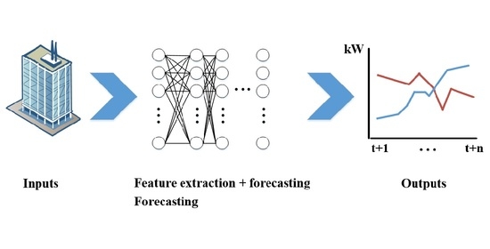
2. Deep Learning Techniques

This section presents the basic definitions, classification and structures of deep learning which have been applied in research. Generally, it was observed that the most popular deep learning-based techniques applied through the review include: autoencoders (AE), recurrent neural networks, and deep neural networks (DNN). Techniques such as deep belief networks, restricted Boltzmann networks, and convolution neural networks have been applied, however, in fewer applications. This section provides a summary of the main deep learning-based techniques applied to date. An in-depth discussion for the techniques and merits of such models is beyond the scope of this work.

2.1. General Overview, Background and Classifications

Deep learning-based techniques have grown in popularity over the past few years and have begun to be applied throughout various research fields. This rise in popularity is a result of: (i) their ability to handle large amounts of data, (ii) their improved feature extraction abilities, and (iii) their improved model performances. In order to provide a general overview of some of the techniques and approaches of deep learning, this paper will begin with a fundamental definition.

Deep learning is a sub-category of machine learning and has been defined as “representation-learning methods with multiple levels of representation, obtained by composing simple but non-linear modules that each transform the representation at one level (starting with the raw input) into a representation at a higher, slightly more abstract level” [3]. Shallow architectures refer to one to three levels of non-linear operations, whereas, deep architectures contain four or more levels [23]. The use of deep learning offers some potential advantages and disadvantages over methods that are more traditional. Firstly, the convention has been for the practitioner to extract good features themselves. This requires a bit of domain expertise and engineering skill. However, deep learning methods can automatically learn using a general learning procedure and thus do not require such domain expertise. This is a key advantage of deep learning, in that feature extraction can becomes automatically learnt [3]. Secondly, deep-learning methods can easily incorporate large amounts of data in order to make accurate predictions. Thus, as big data has become a problem in recent years, deep learning offers a potential solution to overcoming set problem. Thirdly, when compared to conventional ANNs, deep learning models can hold and store more information within the neurons. This can allow learning distributed representation (many-to-many relationships between types of representations) which enable generalization to new combinations of values not explicitly shown in learning data [3]. A disadvantage of deep learning methods is that they are typically difficult to train and contained a large number of hyperparameters.

To the best of the author’s knowledge, there have been three main ways to date in which deep learning-based models have been applied to building energy forecasting:

• Increasing the number of hidden layers in a feed forward neural network/multi-layer perceptron
• Applying some recurrent neural networks (RNN, long-short term memory (LSTM), gated recurrent units (GRU), etc.). Such recurrent neural network models may have a single (or multiple hidden layers), however, they still may be considered a deep learning approach due to their training approaches. Unfolded, which occurs in training of the network, such models are consider networks with very deep structures as information from previous states is passed to current states [24].
• Sequentially coupling of different types of algorithms into an overall structure (for example, coupling a autoencoder for feature extraction with a support vector regression forecasting model)

2.2. Autoencoder

An autoencoder (AE) is a neural network consisting of multiple hidden layers. Each autoencoder consists of an encoder (EN) and a decoder (DE) section. The aim of an autoencoder is to learn the representation for a data set through training in order to reconstruct the output. The EN maps the input into a hidden representation, while the DE maps the hidden representation to an output. Thus, given an input data set X, the encoder maps the data to a representation of a hidden space, h = f(x), while the decoder, then obtains the hidden representation to reconstruct the output g(h) = X′. Training attempts to minimize the difference between the input and output such that X approximately equals X′. Typically AE models are applied for dimensionality reduction/feature detection and encoding features in large datasets. Figure 1 presents the structure of an autoencoder.

2.3. Recurrent Neural Networks

Recurrent neural networks (RNN) are a classification of neural networks specialized in sequence data. A RNN may be distinguishable from a feed forward neural network (FFNN) by the use of a feedback loop connected to their past calculations. The use of a feedback, allows the RNN to contain a ‘memory’ and utilize information from previous outputs over time. Therefore, values calculated for an RNN at time (t) are affected by values the models reached in prior steps (t − 1). With time series data, RNN can learn and model the temporal behaviors exhibited within the time series data and use the feedback connections in order to recall calculations from previous steps. When applied to forecasting energy in buildings, the most prominent RNN networks that have been applied include: the simple recurrent neural network, gated recurrent unit (GRU), and long-short term memory (LSTM) neural networks. GRU and LSTM can be differentiated from the RNN by the use of gates. Gates are applied in order to control information flow and help mitigate short-term memory losses and overcome the vanishing gradient problem. Figure 2 illustrates the internal structure for each of the recurrent models (RNN, GRU, and LSTM).

Where t is the step (t, t − 1, … t − n), x_t is the input vector, h_t is the hidden layer and/or output vector, tanh and σ are activation functions, and c_c is the cell state. A detailed overview of each models functionality, governing equations and merits is presented in references [24,25,26,27].

2.4. Convolutional Neural Networks

Convolutional neural networks (CNN) are a variation of ANN models built to handle larger complexities of data. Specifically, CNN are specialized in processing input data with grid shaped topologies, this has made them suitable for processing 2D images. However, they have achieved promising results with 1D non-image data as well (time series). A CNN model consists of four main parts: (i) the convolutional layer which creates feature maps of the input data (ii) Pooling layers which are applied to reduce the dimensionality of the convoluted feature, (iii) Flattening, which then adjusts the data into a column vector, and (iv) a fully connected hidden layer which calculates the loss function. Figure 3 provides an illustration of a CNN. A detailed overview for the governing equations and merits of a CNN can be found in reference [24].

2.5. Deep Belief Networks

Deep belief networks (DBN) are a type of DNN originally developed by Hilton et al. [28]. DBNs are a variety of algorithms that use probabilities and unsupervised learning approaches to produce outputs. A fundamental aspect of the DBN are the restricted Boltzmann machines (RBM). The RBM is a shallow two-layer neural network used to learn probability distributions over its input data space so that its configuration can exhibit desirable properties [29]. The first layer of the RBM is termed the visible layer, or input layer, while the second is the hidden layer. Figure 4 presents an illustration of the RBM. Applications for the RBM include: dimensionality reduction, regression, classification, collaborative filtering, and feature learning.

In contrast to a RBM, the DBN architecture consists of stacking together multiple RBMs in order to learn more abstract features and information within the input data. Figure 5 provides an illustration for a DBN. Stacking together multiple RBMs can create models sufficiently large, however, the training of such large models may be cumbersome. More information regarding the governing equations and merits of RBMs and DBNs can be seen in references [24,28,29].

2.6. Other

One of the most prominent techniques applied for forecasting energy in buildings has been the deep feed forward neural network (DFFNN). Such models are differentiated from the standard feed forward neural network (FFNN) in that they contain multiple hidden layers in comparison to the standard FFNN. Additional layers are added in order to learn more information from the data. Many other deep learning-based structures have been proposed and applied in research to date. A few additional DL techniques which have not been covered include: stacked extreme learning machines, generative adversarial networks, echo state networks, deconvolutional networks, etc.

3. Current Trends

We reviewed publications over the years 2000 to October 2020. A total number of 63 representative publications were identified and are the basis for this analysis. Appendix A, Appendix B and Appendix C provide the catalogued work. This section discusses the current trends observed over the publication data to date.

3.1. Building Application Level

Data-driven models require validation of methods/algorithms on test beds in order to explore and validate their effectiveness. We categorically breakdown these test beds into four distinct levels: (i) the district level (the load of one or more overall building energy loads aggregated together); (ii) the building level (an overall energy load for a single building); (iii) the sub-meter level (an energy load within a building, less than an overall energy load, that consists of a group of components aggregated together); and (iv) the component level (a single energy load of an appliance/component within a building). The building level may play an influence on the application of the forecasting model along with the amount of data, time steps, and data available. Based on the analysis, the observed breakdown of case studies was found to be: 37% at the district level, 53% for whole buildings, 6% sub-meter, and 4% at the component level. This prevalence towards districts and whole building case studies may be a result of leveraging available data from BAS systems currently installed for district heating/cooling systems and large scale building.

3.2. Data Properties

Data size refers to the amount/length of data used for each case study. As DL-based techniques are proposed to help face big data problems, it was expected that models would be built on years of available data in order to test their performance in handling large volumes of data. The observed breakdown of published work found 17% of models used under six months of data, 22% applied six-months to one-year of data, 58% of papers applied greater than one year of data, and 3% did not specify their data size.

Furthermore, data types were analyzed within this review. Based on review papers [11,16] there are three different types of data typically applied in research: (i) synthetic/simulated data from a building simulation software such as eQuest and EnergyPlus, (ii) real/measurement data, and (iii) benchmark data (e.g., provided from energy prediction competitions). From the analysis conducted it was found that the overwhelming majority, 95%, of case studies have been applied to real/measurement data; followed by 3% for synthetic and 2% for benchmark data.

3.3. Target Variables

Target variable refers to the energy usage the DL-based model has been applied to forecast. We classified the target variables into the following categories (Figure 6): (i) Whole building electrical energy, (ii) Heating energy, (iii) Cooling energy, (iv) Lighting energy, (v) Natural-gas energy, and (vi) Sub-meter/Components energy use within the building. Sub-meter and components include target variables such as chiller electric demand, electric demand of fans, pumps etc.

3.4. Input Types

Input refers to the regressors or features which have been applied as inputs to the forecasting model. Selecting appropriate input data is a crucial step for all energy-based models. For data-driven models, selection of proper inputs is challenging as (i) relevant features are required for accurate forecasts, and (ii) relevant lengths of time are required for each input variable (e.g., t, t − 1, …, t − n). Improper selection of input variables and their lengths may lead to unnecessary computational time, costs, and may result in poor forecasting performance. From the analysis conducted, it was observed that the most popular types of features applied are: (i) environmental data (e.g., outdoor air temperature) and, (ii) historical data (e.g., previous energy usage). Such findings are similar to those found in reference [17] for data driven models. The prevalence towards historical and environmental data could be a result of leveraging available data from sensors and the high correlations between weather conditions and thermal energy requirements for a building. Currently, it is difficult to say which variable is most important as this may be highly dependent on the case study conditions such as location, climate, building type, building purpose etc. Furthermore, common feature selection methods applied include expert knowledge, statistical-based and machine learning techniques. An in-depth analysis of feature selection may be useful, however, it is beyond the scope of this work which will focus on DL-based techniques for feature extraction.

3.5. Temporal Granularity

There are two main types of temporal characteristics of forecasting models: resolution and forecast horizon. Resolution refers to the time step of the data, while forecast horizon refers to the length of time into the future that the forecasting is made. The two temporal granularities can be applied within a variety of ways for forecasting models, e.g., hourly time step data forecasting a horizon of 24 h in advance. The resolutions of the applied models were found to be 1% yearly, 0% monthly, 3% weekly, 6% daily, 41% hourly, and 49% sub-hourly.

Forecast horizon can be classified as long term (greater than three years), medium (two weeks to three years), and short-term (less than two weeks) shown in references [30,31,32]. However, it should be noted that there is no set standard and the boundaries of the previously stated classifications may vary among published articles. Based on the length of the forecast horizon, the application of the model can vary. Medium and long-term forecasts find applications for government standards, scheduled maintenance, and energy saving-based policies. In contrast, short-term forecasting finds more applications in the day-to-day control strategies and energy saving techniques such as demand response, demand side management, optimization and control, etc. Figure 7 provides a breakdown for the forecast horizons of applied research and show the most popular horizons are one hour and 24 h ahead.

4. Deep Learning-Based Applications in Feature Extraction

Feature extraction refers to processes that reduce the dimensionality of the initial raw data set to more manageable groups for processing [33]. Large data sets require a lot of computational resources in order to process, therefore, selecting appropriate and/or combining features can help reduce the computational requirements. For forecasting-based models, this reduction can lead to: accuracy improvement, overfitting risk reductions, and decreased computational resources. For building energy forecasting, the application of DL-based feature extraction techniques are a relatively new approach that have only begun to occur recently. The applications for this model have been growing in recent years due to their quicker computational time and ease of development. Varieties of cases have explored their efficiencies compared with other data-driven models.

In 2017, Fan et al. provided a comparison of four different feature extraction techniques coupled with forecasting models [34]. The feature extraction techniques explored within this paper included: (i) engineering methods, which relied on engineering expertise to select the model, (ii) statistical, which calculated summary statistics of a time series to be used as features, (iii) structural, which transformed the time series to the frequency domain, and (iv) a deep learning autoencoder (AE). Extracted features were coupled with a variety of different algorithms in order to forecast the cooling load for a building with a horizon of 24 h ahead (using 30 min time steps). The authors concluded that features extracted with the DL-based technique usually led to the best forecasting performance, however, further studies are required for testing.

Additionally in 2017, Li et al. compared a DL-based model of combined stacked autoencoders coupled to an extreme learning machine with popular data-driven methods [35]. The forecasting models compared to the DL-based included: a FFNN, SVR, generalized radial basis function neural network, and multiple linear regression. All such models were applied to a case study of a retail building, in order to forecast the whole building energy consumption over a horizon of 60 min ahead at 30 min time steps. The authors observed that the AE coupled to the extreme learning machine provided the lowest forecasting error over their testing data set.

In 2018, Son et al. compared features extracted through three different techniques: original, principal component analysis and an autoencoder [36]. The performance of each technique was then explored as it was coupled to a SVR, FFNN, and a random forest algorithm (RF). The case study for this experiment consisted of clusters of university buildings. The models were trained with 15 min data, had a one-step ahead horizon, and targeted the future electric load of each building cluster. Their observations noted that in 2/3 of the clusters, the coupling of an AE reduced the forecasting error. However, in 1/3 of the clustering the forecasting error was maintained or slightly increased.

In 2019, Liu et al. applied an AE coupled with a deep deterministic policy gradient (DDPG) and compared the models with a SVM and a FFNN [37]. Their experiments were applied to a case study of an office building, targeting the electric demand of a ground source heat pump and forecasting 5 min ahead. The authors observed that the AE-DDPG surpassed the DDPG algorithm and was the highest performer.

In 2020, Moon et al. compared data-driven based techniques in order to forecast the electrical energy consumption of a commercial office building up to 24 h ahead [38]. Two coupled DL models were applied: (i) the proposed model, which consisted of an ensemble of DFFNN, coupled to a principal component regression model, and (ii) an AE–RF model previously shown in reference [36]. The two models were compared to a variety of other data-driven models including: FFNN, persistence, multiple linear regression (MLR), K-nearest neighbors, decision tree, bagging, gradient boosting machine, SVR, and DFFNNs. The experiments showed that the proposed coupled model obtained the best performance in most cases; in the few instances, which it did not, the AE-RF algorithm bested it. Thus, the best performing models in this work were both coupled DL models.

However, while the previous models applied FFNN-based AEs; other authors have begun to apply different neural network structures in AE topologies in order to leverage their characteristics.

In 2018, Rahman et al. applied a LSTM-based AE, the outputs of this were concatenated with the original input, and sequentially passed to a multi-layer neural network [39]. This proposed model was then compared with that of a standard FFNN. The data-driven models were applied over two case studies for medium to long term forecasting. The first case study applied was a public safety building, with a target variable of the overall electricity consumption and a forecast horizon of one week. The second case study consisted of forecasting the electricity consumption of aggregated residential houses over a time horizon of one year. The authors observed that the models performed differently when the data was aggregated or when long-term forecasts were made.

In 2019, Kim and Cho explored the effectiveness of a CNN coupled to a LSTM model in order to forecast the overall electricity consumption of a residential house up to 60 min in advance [40]. The model was compared to DL forecasting models including: LSTM, Bi-directional LSTM, Attention LSTM, and a GRU model. The authors observed that the CNN-LSTM model obtained the highest performance among the DL-based models. Additionally, the authors explored time resolution changes to the data, aggregating minute data into hourly, daily and weekly data for comparison. The results remained consistent and demonstrated that the CNN-LSTM model obtained the best performances over the temporal changes.

Furthermore in 2019, Kim et al. compared a LSTM-CNN model with a MLP, LSTM, and CNN [41]. Three case studies consisted of industrial districts. For each case study, the target variable was the overall electricity load, used 30 min time step data, and a forecast horizon of a day ahead (48 time steps). It was observed that the combined LSTM-CNN model obtained the best performance across all the case studies and varied lengths of training data; however, there was an exception in one scenario, which observed an LSTM model obtaining the best performance.

In 2020, Wang et al. compared the performances of DL models applied to forecast energy loads (electricity, heating, and cooling) for a university campus [42]. The models compared included: a LSTM-FFNN, LSTM-FFNN-GBDT, and LSTM-FFNN-AE-GBDT. The proposed LSTM-FFNN-AE-GBDT model was shown to outperform other advanced models.

Furthermore in 2020, Zhang et al. proposed coupling a deep belief network and an Elman network (ELM) in order to predict the stochastic features of a building energy load [43]. The outputted feature sets of the DBM-ELM model were applied as inputs (along with cyclic features extracted by a spectrum analysis) to an additional ELM in order to generate the overall output forecasts. The proposed DL-based model was then compared to a SVR, ELM, and a DBN model over two different case studies. Both case studies used 30 min time step data to forecast one-step ahead. The experiments demonstrated that the proposed model achieved the best average performance between both case studies.

The published research demonstrates that in most case studies, the inclusion of DL-based feature extraction has led to an increase in forecasting performances when compared to standard data-driven based models. However, few papers have offered comparisons of different DL-based feature extraction techniques against each other.

Fan et al. (2019) compared feature extraction through: (i) principal component analysis, (ii) statistical measures, (iii) an auto-encoder, (iv) a convolutional auto-encoder, and (v) a generative adversarial network [44]. Each feature selection method was then coupled to different forecasting models of: (i) multiple linear regression, (ii) SVR, (iii) FFNN, and (iv) extreme gradient boosting. All combinations of the feature extraction and forecasting models were applied to a case study of an educational building. The case study applied 30 min time step data to forecast one step ahead and 24 h ahead (48 steps ahead). They observed that for a given forecasting model, e.g., SVR, the application of an AE demonstrated improved forecasting performance compared to those of the other feature extraction techniques for the same model. Furthermore, the generative adversarial network AE achieved the highest performance among the AE-based models.

In 2020, Zhang et al. compared stacked DL models including: a LSTM-ANN, a coupled input and forget gate with ANN (CIFG-ANN), and a GRU-ANN [45]. Each recurrent model was applied to extract features from the raw data set, and then coupled to an ANN model to forecast the future cooling demand for a commercial building. The stacked models were compared with non-stacked DL models of a LSTM, CIFG, and a GRU. Furthermore, prominent ML models were applied including an ANN, SVR, RF, and a gradient boosting tree (GBT). Each standard ML model used inputs based on four different types of feature extraction processes. Such processes included domain knowledge, statistical, principal component analysis (PCA), and raw data inputs. Thus, 21 different model types were compared to the stacked DL models. It was observed in their study that the stacked DL models were the top performing models applied and obtain less error than there non-stacked counterpart (LSTM-ANN compared to LSTM) and the standard ML models.

While the results look promising for the inclusion of DL-based feature extraction, there have been a couple instances in which the inclusion has not yielded the top performing algorithm. Nevertheless, in most published cases reviewed in this study, the implementation of DL for feature extraction and coupled to a forecasting algorithm has led to an overall high-performing forecasting model. To date, the applications of DL feature extraction techniques for forecasting building energy are still within their infancy and more research is required in order to compare such models over a variety of different case studies and applications.

5. Deep Learning in Forecasting Models

This section explores how DL-based techniques have been applied as forecasting models over published research. In this discussion, we separate papers based on the categorical breakdown of Section 3.1 (district, whole building, and sub-meter/component).

5.1. Summary of Applications at the District Level

The district level is characterized by multiple whole building energy loads aggregated together. However, not all districts are the same. For this work, we break down the district levels based on their scale and into the following categories: (i) the Sector level, constituting whole sectors (residential, industrial, etc.), (ii) the City level, which contains multiple building types aggregated together, (iii) the Complex level, similar to the city level and containing multiple building types, however, on a smaller scale than a city (e.g., university campus, hospital, etc.), and (iv) the Commercial-Residential level, which group together multiple residential and/or commercial buildings. Such models are differentiated from the complex level in that they only contain residential and/or commercial buildings within the district. In contrast, the complex level can contain a larger variety of building and building types (laboratories, hospitals, libraries, industrial buildings, retail stores etc.). For each level, the applications and DL-based forecasting models will be discussed, highlighting which target variables and the DL models applied.

Table A1. District-level DL papers.

District Level	Year	Application	DNN Type Applied	Target Variable	Reference Number
Sector	2018	Industrial sector	DFFNN/OA	Electricity consumption	[46]
	2019	Residential and Industrial sector	LSTM/DFFNN OA	Natural gas consumption	[47]
	2019	Mackey-Glass Sector	LSTM	Natural gas consumption	[48]
City	2018	Rottne district system Karlshamn district	DFNN/OA	Heating load	[49]
	2019	District system	DFFNN/OA	Heating load	[50]
	2018	Non-residential district	DNARX/OA	Heating load Cooling load	[51]
	2019	District system	DFFNN/LSTM RNN//OA	Heating load	[52]
	2019	District system	LSTM/OA	Heating load	[53]
	2020	District system	LSTM/OA	Heating load	[54]
	2019	London, Karditsa, Hong Kong, Melbourne systems	LSTM/OA	Natural gas	[55]
	2019	Ljubljana	DRNN/OA	Natural gas	[56]
Complex	2018	University	AE-RF/OA	Electric	[36]
	2019	Industrial complex	CNN/RNN/OA	Electric	[41]
	2020	University	LSTM-FFNN	Electric Heating Cooling	[42]
	2019	University	DFFNN	Electric	[57]
	2020	Hospital complex	GMDH	Electric	[58]
	2019	District mixed buildings	DFFNN	Heating	[59]
Commercial-Residential	2016	District heating system for residential and commercial buildings	DFFNN/OA	Heating	[60]
	2018	District heating system for residential and commercial buildings	DFFNN/OA	Heating	[61]
	2017	District residential	DFFNN	Electric	[62]
	2019	District residential (agg.) Residential	LSTM/OA	Electric	[63]
	2019	District Residential (agg) Residential	LSTM/OA	Electric	[64]

OA: Other algorithms/comparison based papers.

in Appendix A provides a summary for the district level applications.

5.1.1. Sector Level

To date, few papers have focused the application of DL-based models at the sector level. However, based on the search conducted, it was observed that one of the first instances for the implementation of DL-based forecasting models was at this level. In 2008, Azadeh et al. applied a DFFNN in order to forecast the annual electricity demand of the industrial sector [46]. The DFFNN model was compared with that of a regression-based model. The results of this experiment showed that the DNN obtained less forecasting error. Since then, published studies have been applied to natural gas-based target variables. In 2019, Laib et al. explored the application of DFFNN and a LSTM models in order to forecast the next day gas consumption for the residential and industrial sectors [47]. Clustering was used to partition the data, after which and MLP would decide on which LSTM model to best handle the forecast. This proposed model was compared to benchmark forecasting models and showed improved accuracy. Furthermore, in 2019 Su et al. explored the effectiveness of stacked LSTMs coupled with LSTM models in order to forecast up to 10 h ahead [48]. Models were tested on two case studies; (i) a benchmark data set, and (ii) a natural gas consumption data set of sectors provided by the US Department of Energy. The experiments demonstrated high accuracy over the forecast horizon.

5.1.2. City Level

City level models have received a lot of attention from the research community. The majority of the applications have been to heating-based target variables [49,50,51,52,53,54] and natural gas-based ([55,56]). Common DL-based models applied to date include the DFFNN and the LSTM.

In 2018, Suryanarayana et al. compared a DFFNN to other popular data-driven models [49]. Their work explored the performances of such models over two case studies for day-ahead forecasting. Their experiments demonstrated that the DNN model obtained a better performance in both case studies that the linear models. While a powerful algorithm, adding additional hidden layers have demonstrated instances in which it was not the top performing algorithm when applied to forecasting district systems. In 2019, Xue et al. compared SVR, DNN, and XGB algorithms in order to forecast the future heating demand of a district heating system up to 24 h ahead [50]. The experimental results showed that while not the top performing model the DNN was a close second. Koschwitz et al. (2018) applied a two-layer nonlinear autoregressive exogenous neural nework (NARx) in order to forecast the heating and cooling loads of a non-residential district [51]. The two-layer model was compared with that of an SVR model and a single layer NARx model. The results demonstrated that NARx models obtained a lower forecasting error, and that the single layer NARx was the top performing model followed closely by the two layer NARx model.

LSTM models have begun to be applied in order to forecast heating demands for district systems and shown promising results in references [52,53,54]. In 2020, Xue et al. compared a variety of different algorithms in order to forecast the heating demand of a district system [54]. Their experiments showed that the LSTM models were among the highest-performing algorithms applied.

When applied to natural gas forecasting of districts, RNN models have shown encouraging results. Wei et al. (2019) explored the application of LSTM for forecasting natural gas consumption of four cities [55]. The LSTM forecasting models were compared with those of MLR, FFNN, and a SVR algorithms. The authors’ experiments demonstrated that the LSTM models obtained higher accuracy than the other data-driven models. Furthermore, in 2019 Hribar et al. compared RNN models to a variety of data-driven based models in order to forecast the natural gas of a city with a one-hour and 24 h ahead horizon [56]. The authors’ experiments observed that the RNN was the most accurate model and that the accuracy of the models were improved with the inclusion of past weather data as an input.

5.1.3. Complex Level

Within the complex level, university campuses/educational districts constitute the majority of the case studies. For such cases, the target variables have ranged from the overall/electric loads (shown in references [36,57]), and multiple energy loads within the district (e.g., electricity, heating, and cooling) [42]. Other notable applications for complex level models have included case studies such as an industrial complex [41], hospital complex [58], and a small eco-district [59]. Due to the small sample pool and lack of comparison-based papers, it is currently still unknown if the applications of DL-based models at this level would lead to any performance improvements. Therefore, it is wise that future research focus on addressing set gaps and exploring the effectiveness of different DL-based models on district complexes.

5.1.4. Commercial-Residential Level

The commercial-residential level is characterized by the grouping of commercial and/or residential buildings together into a single district. To date, there have been two main applications based on the target variables of the applied models: (i) heating ([60,61]) (ii) and the electric demand (shown in references [62,63,64]). The majority of the applied models in research to date have been DFFNN-based. For instance, Yuce et al. (2017) applied deep feed forward neural networks in order to forecast a district of residential buildings [62]. The model proposed in this work used six parallel performing DFFNNs each applied to forecast a specific building, after which the total building cluster would be forecasted. The authors found: (i) the aggregated electricity demand forecast obtained a lower error than the individual buildings, (ii) it was harder to forecast buildings with children under the age of 15 living inside, and (iii) the autumn season contained the largest forecasting errors. LSTM models have shown promising results when applied to commercial and residential level districts. For instance, Kong et al. compared such models in order to forecast the electric loads of residential houses and the aggregation of such loads for the substation level [64]. The LSTM model was compared with other prominent data-driven models and their experimental results demonstrated that the LSTM model obtained the lowest forecasting error.

5.2. Summary of Applications at the Building Level

Building level applications consist of forecasting models applied to estimate the future values of a whole building energy load. In discussing the published research applied at this level; we use the following categorizations: (i) institutional, (ii) commercial, (iii) residential, and (iv) multiple. Here multiple refers to the publications, which applied their experiments across multiple case studies of different building types (e.g., a residential and a commercial building).

Table A2. Building-level DL papers.

Building Level	Year	Application	DNN Type Applied	Target Variable	Reference Number
Institutional	2017	Education	AE-DNN/OA	Cooling	[34]
	2019	Education	CNN/AE-DNN/OA	Cooling	[44]
	2019	Education	RNN/GRU/LSTM	Cooling	[66]
	2020	University	LSTM/DFFNN/OA	Cooling	[67]
	2018	University	DRNN/OA	Heating	[68]
	2019	University	GRU	Electric Cooling	[69]
	2020	University	LSTM/OA	Electric	[70]
	2018	Education	LSTM	Electric	[71]
Commercial	2016	Office	DFFNN/OA	Cooling	[72]
	2018	Office	DBN	Cooling	[73]
	2017	Office	DFNN	Hearing Cooling	[74]
	2020	Complex	DFFNN/OA	Heating	[75]
	2020	N/s Public	LSTM/CIFG/GRU/LSTM-ANN/CIFG-ANN/GRU-ANN/OA	Cooling	[45]
	2017	Retail	Extreme-SAE/OA	Overall	[35]
	2018	Hotel	LSTM	Electric	[79]
	2019	Commercial-N/s	GRU/LSTM/RNN/DFFNN	Electric	[80]
	2020	Commercial	AE-RF/DFFNN/OA	Electric	[38]
	2020	Office	RNN-seq2seq/OA	Electric	[77]
	2020	Office	LSTM/CNN/LSTM-AE/LSTM-dense	Electric	[78]
	2018	N/s Public 1 N/s Public 2	DBN/DBEN/OA	Energy	[43]
	2020	Office	DFFNN	Energy	[76]
Residential	2019	Residential	CNN/RNN/RNN-CNN	Electric	[40]
	2020	Residential	CNN/OA	Electric	[82]
	2016	Residential customer	LSTM	Electric	[83]
	2020	Residential	LSTM/OA	Electric	[84]
	2017	Residential customer	CNN/LSTM/FRBM	Electric	[85]
	2018	Residential	LSTM/GRU/RNN/OA	Electric	[86]
Multiple Case studies	2019	Residential/City Hall/Factory/Hospital	LSTM/MIDAS-LSTM	Electric	[87]
	2016	Public Administration/ Retail/R&D/Business/ Healthcare/ Car part/Electronic/ other manufactures Aggregated loads	RBM/OA	Electric	[88]
	2018	Industrial Commercial	LSTM/OA	Electric	[89]
	2018	Public health Residential Aggregated residential	LSTMAE-ML/OA	Electric	[39]
	2018	Public-N/s	DBM/DEBM/OA	Energy	[43]
	2018	Retail Office	DBM/OA	Overall	[92]
	2019	Hotel Office	LSTM/GRU/OA	Electric	[90]
	2019	Education Commercial	CNN/GRU/OA	Electric	[91]

OA: Other algorithms/comparison based papers.

in Appendix B provides a further description for building level applications.

5.2.1. Institutional

This section discusses papers, which applied a DL-based model to a case study of an institutional building. Based on the search methodology, educational buildings accounted for all the papers in this sub-section. Additional case studies, applied to institutional buildings, were observed; however, they are discussed in Section 5.2.4 as there were multiple case studies within such papers.

It was observed for educational buildings that cooling and electricity usage constituted the majority of target variables of applied research to date. Therefore, there are gaps related to exploring DL forecasting models targeting heating, natural gas, and lighting for institutional and educational-based building applications. A possible explanation for this gap could be the difficulty in obtaining data for some loads (e.g., lighting and/or natural gas [11]). However, heating and lighting loads may constitute a large share of a commercial/institutional buildings overall energy loads (25% for heating and 10% for lighting [65]); therefore, future work may benefit from exploring such avenues.

DL-based forecasting models targeting cooling loads were explored in reference papers [34,44,66,67]. It was observed that the application of a AEs for feature extraction improved the forecasting performance targeting the cooling loads in papers [34,44]. Reference [66] explored the accuracy of RNN, GRU and LSTM-based models for forecasting building cooling loads through direct and recursive approaches. The author’s experiments demonstrated that the direct approach achieved higher accuracy for the RNNs. Reference [67] compared 12 different forecasting approaches for building cooling load applications. Their experiments demonstrated that LSTM and extreme gradient boosting were the most accurate models. Reference [68] applied RNN models to forecast the heating load for various buildings within a university campus. Their experiments observed that the RNN model typically performed better than an MLP-based model for medium to long-term forecasts. With respect to RNNs applied to forecast building thermal energy loads of institutional buildings, they appear to provide improved performances. However, further research is required in order to validate the previously accomplished work over a variety of different case studies.

The application of GRU-based models for forecasting energy use in buildings can be seen in [69]. The authors explored various techniques to impute missing data, after which GRU forecasting models were tested. References [70,71] explored LSTM models targeting electricity load estimations of educational buildings. For instance, in reference paper [70] the authors demonstrated the effectiveness of different LSTM-based models compared with SVR, DBN, and ARIMA-based models.

5.2.2. Commercial

Commercial case studies were found applied to offices [72,73,74,75,76,77,78], retail [35], hotels [79], and non-specified (show in references [38,43,45,80]). Focusing on office buildings, it was observed that thermal loads accounted for approximately half of the case studies applied with a predominance of cooling load applications. DFFNNs have shown promising performance results for forecasting building thermal energy loads. For instance, Bünning et al. applied a DFFNN in order to forecast the heating demand of an office building [75]. The model was compared with other prominent black-box and grey-box based models for a forecast horizon of a day-ahead. The experiment results demonstrated that the DNN model obtained the highest accuracy among the deployed models. However, a 10-layer DFFNN model was applied in reference [72], which provided mixed results. RNN-based models have begun to be applied to commercial-based forecasting and their preliminary applications look positive. For instance, it was observed that LSTM-based models outperformed FFNN models in reference [79]. While such results appear encouraging, further research is required to validate such findings.

5.2.3. Residential

Over published research to date, it was observed that DL models applied for forecasting the energy loads of residential buildings, have strictly targeted electric loads. This lack of applications for energy loads other than electrical may be a result of additional time and costs needed for the data acquisition of thermal, lighting, and/or natural gas loads. Furthermore, forecasting energy loads at such a granular level may be more challenging due to the uncertainty and volatility of the energy loads [81]. The types of DL-based papers applied at the residential level include: CNN [82], LSTM ([83,84]), and comparison-based papers shown in papers [40,85,86].

RNN- and LSTM-based models have achieved the majority of the implementations to date and demonstrated promising results. For instance, Amarasignhe et al. (2017) compared the deep learning techniques of CNN, LSTM, and factorized RBM (FRBM) to conventional ML techniques (ANN, SVM) in order to forecast the electric demand of a building. The forecast horizon was 60 h ahead and used 4 years of training data [85]. Their experiments demonstrated that the DL-based forecasting models obtained less forecasting error when compared with standard machine learning-based techniques; furthermore, the LSTM obtained the smallest error. In addition, Hossen et al. (2018) in a preliminary analysis compared the simple RNN, GRU and LSTM with other data-driven approaches (ARIMA, GLM, RF, SVM, and FFNN) [86]. Their preliminary results demonstrated that all the RNN-based models obtained better forecasting performance than the other data-driven models.

CNN models have shown promising results in their applications to residential energy forecasting models. For instance, in 2020 Estebsari et al. compared CNN-based models to ANN and SVM models for a residential house [82]. Their experiments showed that the CNN-based models achieved a higher accuracy than the SVM and ANN models. Despite their promising results to date, the applications of DL-based techniques for residential energy load forecasting has a relatively small sample size of applications. Thus, further analysis is required.

5.2.4. Multiple Case Studies

This categorical section applies to papers, which have used case studies of different building types within their published work to validate their models; e.g., a residential and an office building as shown in [39]. It is worth noting, that based on the search conducted, it was observed that no paper primarily focused their experiments on a case study of an industrial building. The publications, which did apply their models to industrial buildings, also applied their models to multiple different building types. This can be observed in: (i) reference [87] which applied LSTM-based models to forecast the electrical usage of a residential building, city hall, a hospital building, and a factory; (ii) reference [88] which compared multiple RBM models and data-driven models to forecast the electrical loads of 40 non-residential buildings, of which 15 buildings were manufacturers; and (iii) reference [89] which compared LSTM and other data-driven models to forecast the electrical load of an industrial and commercial building.

Focusing on the type of DL forecasting model, it was observed that LSTM models have received the most applications and demonstrated promising but mixed results. For instance in reference [89], the authors compared an LSTM model with ARIMA, RF, SVR, and ELM. The authors applied their models over a dataset containing 48 different buildings and then averaged their performance results. The experiments demonstrated that the LSTM model had the best performance under each statistical indicator. However, the LSTM model applied in the experiments of reference [90] demonstrated mixed performance results.

CNN-based models have demonstrated potential as well. For example, reference [91] compared CNN- and GRU-based models with a SARIMAX model [91]. Both DL models were compared in a recursive and a multistep ahead forecasting approach. The models were applied to case studies of a grocery store and an academic building targeting the electric demand up to 24 h ahead. The authors’ experiments found that the CNN 24 step models demonstrated the most promising ability in handling the 24 h ahead forecasts.

DBN models have not received much applications, however, they have provided interesting results when applied. For instance, reference [92] compared DBN to other data driven models (FFNN, RBNN, ELM, and SVR) forecasting the energy consumption of a retail store and an office building. The DBN was shown to outperform the other applied algorithms over both case studies.

5.3. Summary of Applications at the Sub-Meter and Component Level

This category refers to publications, which have applied DL-based models to sub-meter and/or components within the building. Typically, models applied at these levels find it more challenging to achieve accurate forecasts due to: (i) a lack of available data, (ii) a larger volatility and uncertainty in their profiles [81], and (iii) component and/or systems may be more sensitive to changes in operation (e.g., HVAC [93] and [94]). Applications of DL-based techniques include: (i) the electric demand of a ground source heat pump [37]; (ii) the electric demand of a ground source heat pump and the HVAC power demand for non-residential buildings [95]; (iii) residential electrical loads and sub-meter loads within a building [96]; (iv) the electric load of appliances and the overall residential building [97]; (v) the electric demand of an HVAC system in an office building [98]; and (vi) the energy consumption forecasting of compressors in a refrigeration system [99].

Table A3. Sub-meter and component-level DL papers.

Year	Application	DNN Type Applied	Target Variable	Reference Number
2019	GSHP- Office	AE-DDPG/OA	Electric	[37]
2014	GSHP HVAC	DFFNN/OA	Electric	[95]
2016	Whole building Sub-meters	CRBM/FCRBM/OA	Electric	[96]
2019	Whole building Appliances	LSTM/OA	Electric	[97]
2020	HVAC total	DDPG/OA	HVAC Electric	[98]
2020	Refrigeration system	LSTM/OA	Compressor Electric	[99]

OA: Other algorithms/comparison-based papers.

provides the list of papers used for this section.

When applied to residential-based buildings and their internal loads, DL models have shown robust results. For instance, conditioned and factorized RBM models were compared to an RNN, ANN and SVM model in reference [96]. The authors applied the data-driven models to forecast the electric demand of the house and sub-meters varying the forecast horizon. Their experimental results demonstrated that the RBM models outperformed the other data-driven models applied. The authors also observed that the RNN was fast in terms of training, however, not stable in its performance.

However, RNN models have shown promising results in other applications. For instance, reference [99] applied an LSTM model for one-step ahead forecasting of the compressors energy consumption. The RNN model was compared with other popular forecasting models including: ARMA, ARIMA, and FFNN. Their experiments demonstrated that the LSTM model obtained a higher performance than the other applied models.

Due to the small sample size of papers over different target variables, it is difficult to generalize if DL models may help when applied at such levels. While the published work to date looks promising, future studies are required in order to verify the performance of DL models across different sub-meter loads and components within buildings. However, such research is vital as sub-level components can contribute significant portions to a buildings overall electric demand. For example, the HVAC system of a commercial building can contribute 19–76% of the buildings overall electrical demand (depending on the type of commercial building) [65].

6. Discussion and Remarks

Deep learning techniques and approaches have been growing rapidly in recent years due to their capabilities of handling large amounts of data and improved performance results. To date, there is already quite a large amount of literature about their applications in forecasting building energy. We have observed that to date, most DL-based models have been applied to whole building and district energy case studies, target the overall energy loads, with a short term forecast horizon (a day ahead and hour ahead the most common horizons). The deep feed-forward neural network and the LSTM model appear to consist of the majority of the DL techniques applied to date. Furthermore, when assessing performance improvements from the application of DL-based techniques, it was observed that the inclusion of a DL-based technique applied for feature extraction purposes typically led to an increase in forecasting performance compared to other ML-based techniques. However, it did not in a few instances. Moreover, when applied as forecasting models, similar observations were observed. Despite the promising results observed, there are significant challenges which need addressing.

6.1. Challenges

While the application of DL-based techniques for forecasting building energy loads are still in their infancy, there are many exciting and new challenges to be faced. We breakdown the largest observed challenges into two main categories: (i) challenges facing the research community and, (ii) technical challenges facing DL-based techniques. Beginning with the challenges facing the research community the following was observed:

• The majority of papers have used proprietary non-published datasets. Similarly, this observation was noticed in review paper [17] for data-driven models as a whole. The overuse of proprietary data makes it challenging to reproduce results, to do comparison-based studies, and/or to build upon the research of others.
• With a growing amount of publishers and journals, there is no standard of forecasting model information required within each journal article. This lack of a standard results in:
• (I). Missing descriptions of components/or techniques applied within their research. For instance, it was observed that a few papers did not specify their forecast horizons, hyperparameter tuning approach, etc.
• (II). Varied use of performance metrics applied within each published work. For instance, the mean absolute percent error is the most commonly applied performance metric throughout research stated in references [11] and [14]. However, it is not always applied within research and sometimes authors would deploy different metrics or modified version of the metrics.
• (III). The use of ambiguous terminology was often found in research further clouding issues.

Turning the attention towards DL-based models, there are a few big challenges noticed over the published research to date. These include:

• There is a lack of general guidelines for the development and testing of DL-based models. The lack of guidelines makes it significantly more challenging in order to develop, apply, and compare such models. For instance, it was observed that the majority of papers tuned their hyperparameters through trial and error. Having an automated procedure and/or guidelines would help with the reproducibility of results and the construction of various models.
• While the models have shown potential for improving forecasting performance at a variety of levels, they come with a tradeoff of increased model complexity and training times compared with standard ML approaches.
• Finally, it was observed there was a lack of practical applications/implementation of the models and sensitivity analysis of the models applied.

The establishment of guidelines for DL models would help future researchers by providing them with a standardized set of criteria to build upon and compare models. This may in turn allow generalizations to be found in a timelier manner.

6.2. Potential Future Research Directions

The future directions of DL-based techniques with respect to their applications for forecasting building energy include:

• The enrichment of DL techniques across a variety of building types, with an emphasis on comparison-based papers and studies.
• Application of DL models to case studies which have not received much attention: lightning, natural gas, medium to long-term forecast horizons, sub-meter/components etc.
• Application of DL grey-box models applied to various case studies.
• Exploration of the sensitivity and uncertainty of the DL models
• The establishment of guidelines for DL model development; including automation of the hyperparameter selection
• The establishment of scalable DL-based models which can be developed and tuned in a timely manner for practical implementations across different buildings and systems
• The development of robust models which can continue to provide accurate forecasts in the event of changes of operation, sensor failure, etc.
• Implementation of the novel DL-based techniques with real applications and control systems e.g., model predictive controllers, or demand side management scheduling, optimization etc.

7. Conclusions

The purpose of this work was to provide a review of deep learning-based techniques applied to forecasting energy usage in buildings. First, fundamental definitions and classifications for DL-based models are presented, which were then followed by an overview of some of the most prominent techniques. Next, this paper provided a breakdown of current trends observed over published research. After which, the feasibility of DL models applied for feature extraction and as forecasting models was discussed. Finally, this paper presented several challenges faced for such models and future directions of DL-based research. Based on our review, it was observed that when applied to feature extraction, DL-based techniques have shown to achieve a higher performance results compared with other methods. Furthermore, similar results were observed when the DL-based techniques were applied as forecasting models. It is difficult to assess which DL-based technique achieved the most promising results, as there are a lack of comparison-based papers among DL-based techniques. However, the results achieved to date look promising and future work should expand on the current body of knowledge.

Despite the rapid expansion of papers and case studies over the past few years, there remain many challenges and work to be accomplished. Such work can include: the application of DL-based techniques on target variables and case studies not commonly applied, comparison of DL-based techniques over a variety of case studies, and the implementation of such models in practical applications. Forecasting models play a fundamental role in many applications for energy improvements and management. Such applications can include but are not limited to: demand side management, model predictive control, fault detection and diagnosis, optimization, scheduled maintenance and planning. The discussion and results of this article may help energy modelers, professionals, and researchers to decide which DL-based tools to select and consequently assist in the development of the field.

References

1. IEA. Buildings, IEA. Available online: https://www.iea.org/topics/buildings (accessed on 2 July 2020).
2. American Society of Heating; Refrigerating and Air-Conditioning Engineers. ASHRAE Handbook: Fundamentals; American Society of Heating, Refrigerating and Air-Conditioning Engineers: Atlanta, GA, USA, 2017. [Google Scholar]
3. LeCun, Y.; Bengio, Y.; Hinton, G. Deep learning. Nature 2015, 521, 436–444. [Google Scholar] [CrossRef] [PubMed]
4. Zhao, H.; Magoules, F. A review on the prediction of building energy consumption. Renew. Sustain. Energy Rev. 2012, 16, 3586–3592. [Google Scholar] [CrossRef]
5. Kumar, R.; Aggarwal, R.; Sharma, J. Energy analysis of a building using artificial neural networks: A review. Energy Build. 2013, 65, 352–358. [Google Scholar] [CrossRef]
6. Ahmad, M.; Hassan, M.; Abdullah, H.; Rahman, F.; Hussin, H.; Abdullah, H.; Saidur, R. A review on applications of ANN and SVM for building electrical energy consumption forecasting. Renew. Sustain. Energy Rev. 2014, 33, 102–109. [Google Scholar] [CrossRef]
7. Li, X.; Wen, J. Review of building energy modeling for control and operation. Renew. Sustain. Energy Rev. 2014, 37, 517–537. [Google Scholar] [CrossRef]
8. Wang, Z.; Srinivasan, R. A review of artificial intelligence based building energy use prediction: Contrasting the capabilities of single and ensemble prediction models. Renew. Sustain. Energy Rev. 2017, 75, 796–808. [Google Scholar] [CrossRef]
9. Daut, M.; Hassan, M.; Abdullas, H.; Rahman, H.; Abdullah, M.; Hussin, F. Building electrical energy consumption forecasting analysis using conventional and artificial intelligence methods: A review. Renew. Sustain. Energy Rev. 2017, 70, 1108–1118. [Google Scholar] [CrossRef]
10. Deb, C.; Zhang, F.; Yang, J.; Lee, S.; Shah, K. A review on time series forecasting techniques for building energy consumption. Renew. Sustain. Energy Rev. 2017, 74, 902–924. [Google Scholar] [CrossRef]
11. Amasyali, K.; El-Gohary, N. A review of data driven building energy consumption prediction studies. Renew. Sustain. Energy Rev. 2018, 81, 1192–1205. [Google Scholar] [CrossRef]
12. Wei, Y.; Zhang, X.; Shi, Y.; Xia, L.; Pan, S.; Wu, J.; Han, M.; Zhao, X. A review of data-driven approaches for prediction and classification of building energy consumption. Renew. Sustain. Energy Rev. 2018, 82, 1027–1047. [Google Scholar] [CrossRef]
13. Ahmad, T.; Chen, H.; Guo, Y.; Wang, J. A comprehensive overview on the data driven and large scale based approaches for forecasting of building energy demand: A review. Energy Build. 2018, 165, 301–320. [Google Scholar] [CrossRef]
14. Bourdeau, M.; Zhai, X.; Nefzaoui, E.; Guo, X.; Chatellier, P. Modeling and forecasting building energy consumption: A review of data driven techniques. Sustain. Cities Soc. 2019, 48, 101533. [Google Scholar] [CrossRef]
15. Mohandes, S.; Zhang, X.; Mahdiyar, A. A comprehensive review on the application of artificial neural networks in building energy analysis. Neurocomputing 2019, 340, 55–75. [Google Scholar] [CrossRef]
16. Runge, J.; Zmeureanu, R. Forecasting energy use in buildings using artificial neural networks: A review. Energies 2019, 12, 3254. [Google Scholar] [CrossRef] [Green Version]
17. Sun, Y.; Haghighat, F.; Fung, B. A review of the-state-of-the-art in data-driven approaches for building energy prediction. Energy Build. 2020, 221, 110022. [Google Scholar] [CrossRef]
18. Wang, H.; Lei, Z.; Zhang, X.; Zhou, B.; Peng, J. A review of deep learning for renewable energy forecasting. Energy Convers. Manag. 2019, 198, 111799. [Google Scholar] [CrossRef]
19. Aslam, Z.; Javaid, N.; Ahmad, A.; Ahmed, A.; Gulfam, S. A combined deep learning and ensemble learning methodology to avoid electricity theft in smart grids. Energies 2020, 13, 5599. [Google Scholar] [CrossRef]
20. Marcjasz, G. Forecasting electricity prices using deep neural networks: A robust hyper-parameter selection scheme. Energies 2020, 13, 4605. [Google Scholar] [CrossRef]
21. Tao, Q.; Liu, F.; Li, Y.; Sidorov, D. Air pollution forecasting using a deep learning model based on 1D convnets and bidirectional GRU. IEEE Access 2019, 7, 6690–76698. [Google Scholar] [CrossRef]
22. Liu, M.; Li, G.; Li, J.; Zhu, X.; Yao, Y. Forecasting the price of Bitcoin using deep learning. Financ. Res. Lett. 2020. [Google Scholar] [CrossRef]
23. Bengio, Y. Learning deep architectures for AI. Found. Trends Mach. Learn. 2009, 2, 1–127. [Google Scholar] [CrossRef]
24. Goodfellow, I.; Bengio, Y.; Courville, A. Deep Learning; MIT Press: Cambridge, MA, USA, 2016. [Google Scholar]
25. Olah, C. Understanding LSTM Networks. 27 August 2015. Available online: https://colah.github.io/posts/2015-08-Understanding-LSTMs/ (accessed on 2 July 2020).
26. Amidi, A.; Amidi, S. Recurrent Neural Networks Cheatsheet. Standford University. Available online: https://stanford.edu/~shervine/teaching/cs-230/cheatsheet-recurrent-neural-networks (accessed on 15 July 2020).
27. Wang, H.; Raj, B. On the Origin of Deep Learning. arxiv 2017, arXiv:1702.07800. [Google Scholar]
28. Hinton, G.; Osindero, S.; Yee-Whye, T. A Fast learning algorithm for deep belief nets. Neural Comput. 2006, 18, 1527–1554. [Google Scholar] [CrossRef] [PubMed]
29. University of Toronto. CSC2535 Lectures. 16 July 2020. Available online: http://www.cs.toronto.edu/~hinton/csc2535/lectures.html (accessed on 20 July 2020).
30. Hong, T.; Fan, S. Probabilistic electric load forecasting: A tutorial review. Int. J. Foreast. 2016, 32, 914–938. [Google Scholar] [CrossRef]
31. Hong, T.; Shahidehpour, M. Load Forecasting: Case Study; United States Department of Energy: Washington, DC, USA, 2015. [Google Scholar]
32. Song, K.; Baek, Y.; Hong, D.; Jang, G. Short-term load forecasting for the holidays using fuzzy linear regression method. IEEE Trans. Power Syst. 2005, 20, 96–101. [Google Scholar] [CrossRef]
33. Alpaydin, E. Introduction to Machine Learning, 3rd ed.; PHI Learning Pvt. Ltd.: Delhi, India, 2014. [Google Scholar]
34. Fan, C.; Xiao, F.; Zhao, Y. A short-term building cooling load prediction method using deep learning algorithms. Appl. Energy 2017, 195, 222–233. [Google Scholar] [CrossRef]
35. Li, C.; Ding, Z.; Zhao, D.; Yi, J.Y.; Zhang, G. Building energy consumption prediction: An extreme deep learning approach. Energies 2017, 10, 1525. [Google Scholar] [CrossRef]
36. Son, M.; Moon, J.; Jung, S.; Hwang, E. A Short-Term Load Forecasting Scheme Based on Auto-Encoder and Random Forest. In Applied Physics, System Science and Computers III; APSAC 2018. Lecture Notes in Electrical Engineering; Ntalianis, K., Vachtsevanos, G., Borne, P., Croitoru, A., Eds.; Springer: Cham, Switzerland, 2018; Volume 574. [Google Scholar] [CrossRef]
37. Liu, T.; Xu, C.; Guo, Y.; Chen, H. A novel deep reinforcement learning based methodology for short-term HVAC system energy consumption prediction. Int. J. Refrig. 2019, 107, 39–51. [Google Scholar] [CrossRef]
38. Moon, J.; Jung, S.; Rew, J.; Rho, S.; Hwang, E. Combination of short-term load forecasting models based on a stacking ensemble approach. Energy Build. 2020, 216, 109921. [Google Scholar] [CrossRef]
39. Rahman, A.; Srikumar, V.; Smith, A. Predicting electricity consumption for commercial and residential buildings using deep recurrent neural networks. Appl. Energy 2018, 212, 372–385. [Google Scholar] [CrossRef]
40. Kim, T.; Cho, S. Predicting residential energy consumption using CNN-LSTM neural networks. Energy 2019, 182, 72–81. [Google Scholar] [CrossRef]
41. Kim, J.; Moon, J.; Hwang, E.; Kang, P. Recurrent inception convolution neural network for multi short-term load forecasting. Energy Build. 2019, 194, 328–341. [Google Scholar] [CrossRef]
42. Wang, S.; Wang, S.; Chen, H.; Gu, Q. Multi-energy load forecasting for regional integrated energy systems considering temporal dynamic and coupling characteristics. Energy 2020, 195, 116964. [Google Scholar] [CrossRef]
43. Zhang, G.; Tian, C.; Li, C.; Zhang, J.; Zuo, W. Accurate forecasting of building energy consumption via a novel ensembled deep learning method considering the cyclic feature. Energy 2020, 201, 117531. [Google Scholar] [CrossRef]
44. Fan, C.; Sun, Y.; Zhao, Y.; Song, M.; Wang, J. Deep learning-based feature engineering methods for improved building energy prediction. Appl. Energy 2019, 240, 35–45. [Google Scholar] [CrossRef]
45. Zhang, C.; Li, J.; Zhao, Y.; Li, T.; Chen, Q.; Zhang, X. A hybrid deep learning-based method for short-term building energy load prediction combined with an interpretation process. Energy Build. 2020, 225, 110301. [Google Scholar] [CrossRef]
46. Azadeh, A.; Ghaderi, S.; Sohrabkhani, S. Annual electricity consumption forecasting by neural network in high energy consuming industrial sectors. Energy Convers. Manag. 2008, 49, 2272–2278. [Google Scholar] [CrossRef]
47. Laib, O.; Khadir, M.; Mihaylova, L. Toward efficient energy systems based on natural gas consumption prediction with LSTM Recurrent Neural Networks. Energy 2019, 177, 530–542. [Google Scholar] [CrossRef]
48. Su, H.; Zio, E.; Zhang, J.; Xu, M.; Li, X.; Zhang, Z. A hybrid hourly natural gas demand forecasting method based on the integration of wavelet transform and enhanced Deep-RNN model. Energy 2019, 178, 585–597. [Google Scholar] [CrossRef] [Green Version]
49. Suryanarayana, G.; Lago, J.; Geysen, D.; Aleksiejuk, P.; Johansson, C. Thermal load forecasting in district heating networks using deep learning and advanced feature selection methods. Energy 2018, 157, 141–149. [Google Scholar] [CrossRef]
50. Xue, P.; Jiang, Y.; Zhou, Z.; Chen, X.; Fang, X.; Liu, J. Multi-step ahead forecasting of heat load in district heating systems using machine learning algorithms. Energy 2019, 188, 116085. [Google Scholar] [CrossRef]
51. Koschwitz, D.; Frisch, J.; Treeck, C.V. Data-driven heating and cooling load predictions for non-residential buildings based on support vector machine regression and NARX Recurrent Neural Network: A comparative study on district scale. Energy 2018, 165, 134–142. [Google Scholar] [CrossRef]
52. Gong, M.; Zhou, H.; Wang, Q.; Wang, S.; Yang, P. District heating systems load forecasting: A deep neural networks model based on similar day approach. Adv. Build. Energy Res. 2019, 14, 372–388. [Google Scholar] [CrossRef]
53. Xue, G.; Pan, Y.; Lin, T.; Song, J.; Qi, C.; Wang, Z. District heating load prediction algorithm based on feature fusion LSTM model. Energies 2019, 12, 2122. [Google Scholar] [CrossRef] [Green Version]
54. Xue, G.; Qi, C.; Li, H.; Kong, X.; Song, J. Heating load prediction based on attention long short term memory: A case study of Xingtai. Energy 2020, 203, 117846. [Google Scholar] [CrossRef]
55. Wei, N.; Li, C.; Peng, X.; Li, Y.; Zeng, F. Daily natural gas consumption forecasting via the application of a novel hybrid model. Appl. Energy 2019, 250, 358–368. [Google Scholar] [CrossRef]
56. Hribar, R.; Potocnik, P.; Silc, J.; Papa, G. A comparison of models for forecasting the residential natural gas. Energy 2019, 167, 511–522. [Google Scholar] [CrossRef]
57. Dagdougui, H.; Bagheri, F.; Le, H.; Dessaint, L. Neural network model for short-term and very-short-term load forecasting in district buildings. Energy Build. 2019, 203, 109408. [Google Scholar] [CrossRef]
58. Zor, K.; Celik, O.; Timur, O.; Teke, A. Short-term building electrical energy consumption forecasting by employing gene expression programming and GMDH networks. Energies 2020, 13, 1102. [Google Scholar] [CrossRef] [Green Version]
59. Reynolds, J.; Ahmad, M.; Rezgui, Y.; Hippolyte, J. Operational supply and demand optimisation of a multi-vector district energy system using artificial neural networks and a genetic algorithm. Appl. Energy 2019, 235, 699–713. [Google Scholar] [CrossRef]
60. Idowu, S.; Saguna, S.; Ahlund, C.; Schelen, O. Applied machine learning: Forecasting heat load in district heating system. Energy Build. 2016, 133, 478–488. [Google Scholar] [CrossRef]
61. Geysen, D.; de Somer, O.; Johansson, C.; Brage, J.; Vanhoudt, D. Operational thermal load forecasting in district heating networks using machine learning and expert advice. Energy Build. 2018, 162, 144–153. [Google Scholar] [CrossRef]
62. Yuce, B.; Mourshed, M.; Rezgui, Y. A smart forecasting approach to district energy management. Energies 2017, 8, 1073. [Google Scholar] [CrossRef] [Green Version]
63. Vesa, A.V.; Ghitescu, N.; Pop, C.; Antal, M.; Cioara, T.; Anghel, I.; Salomie, I. A stacking multi-learning ensemble model for predicting near real time energy consumption demand of residential buildings. In Proceedings of the IEEE 15th International Conference on Intelligent Computer Communication and Processing (ICCP), Cluj-Napoca, Romania, 5–7 September 2019. [Google Scholar]
64. Kong, W.; Dong, Y.; Jia, Y.; Hill, D.; Xu, Y.; Zhang, Y. Short-term residential load forecasting based on lstm recurrent neural network. IEEE Trans. Smart Grid 2019, 10, 841–851. [Google Scholar] [CrossRef]
65. U.S. Energy Information Agency. Commercial Building Energy Consumption Survery. 18 March 2016. Available online: https://www.eia.gov/consumption/commercial/reports/2012/energyusage/ (accessed on 1 July 2020).
66. Fan, C.; Wang, J.; Gang, W.; Li, S. Assessment of deep recurrent neural network-based strategies for short-term building energy predictions. Appl. Energy 2019, 236, 700–710. [Google Scholar] [CrossRef]
67. Wang, Z.; Hong, T.; Piette, M. Building thermal load prediction through shallow machine learning and deep learning. Appl. Energy 2020, 263, 114683. [Google Scholar] [CrossRef] [Green Version]
68. Rahman, A.; Smith, A.D. Predicting heating demand and sizing a stratified thermal storage tank using deep learning algorithms. Appl. Energy 2018, 228, 108–121. [Google Scholar] [CrossRef]
69. Yang, J.; Tan, K.; Santamouris, M.; Lee, S. Building energy consumption raw data forecasting using data cleaning and deep recurrent neural networks. Buildings 2019, 9, 204. [Google Scholar] [CrossRef] [Green Version]
70. Somu, N.; Raman, G.; Ramamritham, K. A hybrid model for building energy consumption forecasting using long short term memory networks. Appl. Energy 2020, 261, 114131. [Google Scholar] [CrossRef]
71. Nichiforov, C.; Stamatescu, G.; Stamatescu, I.; Calofir, V.; Fagarasan, I.; Iliescu, S. Deep learning techniques for load forecasting in large commercial buildings. In Proceedings of the 22nd International Conference on System Theory, Control and Computing (ICSTCC), Sinaia, Romania, 10–12 October 2018. [Google Scholar]
72. Li, X.; Wen, J.; Bai, E.W. Developing a whole building cooling energy forecasting model for on-line operation optimization using proactive system identification. Appl. Energy 2016, 164, 69–88. [Google Scholar] [CrossRef]
73. Fu, G. Deep belief network based ensemble approach for cooling load forecasting of air-conditioning system. Energy 2018, 148, 269–282. [Google Scholar] [CrossRef]
74. Gunay, B.; Shen, W.; Newsham, G. Inverse blackbox modeling of the heating and cooling load in office buildings. Energy Build. 2017, 142, 200–210. [Google Scholar] [CrossRef] [Green Version]
75. Bunning, F.; Heer, P.; Smith, R.; Lygeros, J. Improved day ahead heating demand forecasting by online correction methods. Energy Build. 2020, 211, 109821. [Google Scholar] [CrossRef] [Green Version]
76. Luo, X.; Oyedele, L.; Ajayi, A.; Akinade, O.; Owolabi, H.; Ahmed, A. Feature extraction and genetic algorithm enhanced adaptive deep neural network for energy consumption prediction in buildings. Renew. Sustain. Energy Rev. 2020, 131, 109980. [Google Scholar] [CrossRef]
77. Skomski, E.; Lee, J.; Kim, W.; Chandan, V.; Katipamula, S.; Hutchinson, B. Sequence-to-sequence neural networks for short-term electrical load forecasting in commercial office buildings. Energy Build. 2020, 226, 110350. [Google Scholar] [CrossRef]
78. Gao, Y.; Ruan, Y.; Fang, C.; Yin, S. Deep learning and transfer learning models of energy consumption forecasting for a building with poor information data. Energy Build. 2020, 223, 110156. [Google Scholar] [CrossRef]
79. Yong, Z.; Xiu, Y.; Chen, F.; Pengfei, C.; Binchao, C.; Taijie, L. Short-term building load forecasting based on similar day selection and LSTM network. In Proceedings of the IEEE Conference on Energy Internet and Energy System Integration, Beijing, China, 20–22 October 2018. [Google Scholar]
80. Sehovac, L.; Nesen, C.; Grolinger, K. Forecasting building energy consumption with deep learning: A sequence to sequence approach. In Proceedings of the IEEE International Congress on Internet of Things (ICIOT), Milan, Italy, 8–13 July 2019. [Google Scholar]
81. Stephen, B.; Tang, X.; Harvey, P.; Galloway, S.; Jennett, K. Incorporating practice theory in sub-profile models for short term aggregated residential load forecasting. IEEE Trans. Smart Grid 2017, 8, 1591–1598. [Google Scholar] [CrossRef] [Green Version]
82. Estebsari, A.; Rajabi, R. Single residential load forecasting using deep learning and image encoding techniques. Electronics 2020, 9, 68. [Google Scholar] [CrossRef] [Green Version]
83. Marino, D.; Amarasinghe, K.; Manic, M. Building energy load forecasting using deep neural networks. In Proceedings of the IEEE Industrial Electronics Society, Florence, Italy, 24–27 October 2016. [Google Scholar]
84. Shah, M.A.; Sajjad, I.A.; Khan, M.F.N.; Iqbal, M.M.; Liaqat, R.; Shah, M. Short-term meter level load forecasting of residential customers based on smart meter’s data. In Proceedings of the International Conference on Engineering and Emerging Technologies (ICEET), Lahore, Pakistan, 22–23 February 2020. [Google Scholar]
85. Amarasinghe, K.; Marino, D.L.; Manic, M. Deep neural networks for energy load forecasting. In Proceedings of the 2017 IEEE 26th International Symposium on Industrial Electronics (ISIE), Edinburgh, UK, 19–21 June 2017. [Google Scholar]
86. Hossen, T.; Nair, A.; Chinnathambi, R.; Ranganathan, P. Residential load forecasting using deep neural networks (DNN). In Proceedings of the 2018 North American Power Symposium (NAPS), Fargo, ND, USA, 9–11 September 2018. [Google Scholar]
87. Choi, E.; Cho, S.; Kim, D. Power demand forecasting using long short-term memory (LSTM) deep-learning model for monitoring energy sustainability. Sustainability 2020, 3, 1109. [Google Scholar] [CrossRef] [Green Version]
88. Ryu, S.; Noh, J.; Kim, H. Deep neural network based demand side short term load forecasting. Energies 2017, 10, 3. [Google Scholar] [CrossRef]
89. Jiao, R.; Zhang, T.; Jiang, Y.; He, H. Short-term non-residential load forecasting based on multiple sequences LSTM recurrent neural network. IEEE Access 2018, 6, 59438–59448. [Google Scholar] [CrossRef]
90. Shan, S.; Cao, B.; Wu, Z. Forecasting the short-term electricity consumption of building using a novel ensemble model. IEEE Access 2019, 7, 88093–88106. [Google Scholar] [CrossRef]
91. Cai, M.; Pipattanasompom, M.; Rahman, S. Day-ahead building-level load forecasts using deep learning vs. traditional time-series techinques. Appl. Energy 2019, 1078–1088. [Google Scholar] [CrossRef]
92. Li, C.; Ding, Z.; Yi, J.; Lv, Y.; Zhang, G. Deep belief network based hybrid model for building energy consumption prediction. Energies 2018, 11, 242. [Google Scholar] [CrossRef] [Green Version]
93. Le Cam, M.; Daoud, A.; Zmeureanu, R. Forecasting electric demand of supply fan using data mining techniques. Energy 2016, 101, 541–557. [Google Scholar] [CrossRef]
94. Runge, J.; Zmeureanu, R.; Le Cam, M. Hybrid short-term forecasting of the electric demand of supply fans using machine learning. J. Build. Eng. 2020, 29, 101144. [Google Scholar] [CrossRef]
95. Schachter, J.; Mancarella, P. A short-term load forecasting model for demand response applications. In Proceedings of the 11th International Conference on the European Energy Market (EEM14), Krakow, Poland, 28–30 May 2014. [Google Scholar]
96. Mocanu, E.; Nguyen, P.; Gibescu, M.; Kling, W. Deep learning for estimating building energy consumption. Sustain. Energy Grids Netw. 2016, 6, 91–99. [Google Scholar] [CrossRef]
97. Imani, M.; Ghassemian, H. Residential load forecasting using wavelet and collaborative representation transforms. Appl. Energy 2019, 253, 113505. [Google Scholar] [CrossRef]
98. Liu, T.; Tan, Z.; Xu, C.; Chen, H.; Li, Z. Study on deep reinforcement learning techniques for building energy consumption forecasting. Energy Build. 2020, 208, 109675. [Google Scholar] [CrossRef]
99. Wang, J.; Du, Y.; Wang, J. LSTM based long-term energy consumption prediction with periodicity. Energy 2020, 197, 117197. [Google Scholar] [CrossRef]
Figure 1. Example structure for an under-complete autoencoder.
Energies 14 00608 g001
Figure 2. Recurrent neural network types.
Energies 14 00608 g002
Figure 3. Example structure for a convolutional neural network.
Energies 14 00608 g003
Figure 4. Example structure of a restricted Boltzmann machine.
Energies 14 00608 g004
Figure 5. Example of a structure for a deep belief network.
Energies 14 00608 g005
Figure 6. Compositional breakdown for target variables deep learning (DL)-based models.
Energies 14 00608 g006
Figure 7. Compositional breakdown of the forecast horizons.
Energies 14 00608 g007
Publisher’s Note: MDPI stays neutral with regard to jurisdictional claims in published maps and institutional affiliations.