Application of Support Vector Machine Modeling for the Rapid Seismic Hazard Safety Evaluation of Existing Buildings

Abstract

The economic losses from earthquakes tend to hit the national economy considerably; therefore, models that are capable of estimating the vulnerability and losses of future earthquakes are highly consequential for emergency planners with the purpose of risk mitigation. This demands a mass prioritization filtering of structures to identify vulnerable buildings for retrofitting purposes. The application of advanced structural analysis on each building to study the earthquake response is impractical due to complex calculations, long computational time, and exorbitant cost. This exhibits the need for a fast, reliable, and rapid method, commonly known as Rapid Visual Screening (RVS). The method serves as a preliminary screening platform, using an optimum number of seismic parameters of the structure and predefined output damage states. In this study, the efficacy of the Machine Learning (ML) application in damage prediction through a Support Vector Machine (SVM) model as the damage classification technique has been investigated. The developed model was trained and examined based on damage data from the 1999 Düzce Earthquake in Turkey, where the building’s data consists of 22 performance modifiers that have been implemented with supervised machine learning.

1. Introduction

The world has experienced innumerable catastrophic earthquakes in the history of mankind that led to enormous counts of fatalities and acute property damage. Old structures in service, structures with historical heritage, highly important buildings, and buildings not compliant with current seismic codes are the most vulnerable to seismic damage. In that case, a seismic structural prioritization is credibly the best way to adopt prevention or be prepared with post-disaster management schemes. Therefore, proposing a method called Rapid Visual Screening (RVS) helps to determine the damage index for different types of structures [1,2]. Sinha and Goyal [3] have provided a very effective and concise discussion as a motivation for a novice reader. The demand for an elementary and rapid vulnerability assessment was identified first in the United States of America and, therefore, the first method for RVS was proposed in 1988 as “Rapid Visual Screening of Buildings for Potential Seismic Hazards: A Handbook” [4], which was later revised in 2002 incorporating the latest research advancements in seismic sciences. This was further applied by other countries while adopting their local conditions, modifications, and considerations [5]; for instance, Indian RVS (IITK-GSDMA) [6] or Philippine RVS [7]. RVS typically involves a walk down survey to record the seismic parameters of structures through visual inspection. For this purpose, an experienced evaluator is needed with the set of conventional data sheets to perform this process. RVS is an effective mechanism to filter the weak structures through faster implementation and with concise steps, which evaluates the wide-spread areas in a shorter time span. RVS is a score-based system, in which the final performance score shall be obtained through fundamental computations. The cutoff performance score shall be predefined for each approach, i.e., Federal Emergency Management Agency (FEMA) and the structures which fail to achieve the cutoff score shall be further treated with second and third stage detailed evaluation. Seismic vulnerability assessment is conducted in three steps [8]: Walk down the survey, preliminary assessment, and detailed estimation. The initial step depicts a walk down an investigation that includes the screening of seismically vulnerable structures. Here, it can be observed that the structures that are unable to meet the expectations can be filtered and proceed to the next investigation. In the second step, a comprehensive work shall be conducted by investigating various components of the structure such as the existing ground conditions, quality of the material used, the state of building elements, etc. Furthermore, the structures which require more attention can be considered for the final step. Here, the implementation of process, which can define the structural behavior under seismic excitations, known as nonlinear dynamic structural analysis, shall be conducted [9].

Extensive research in incorporating several methodologies into RVS, for instance, statistical methods [10,11], Artificial Neural Network (ANN) [12,13,14], Multi-criteria decision making [15], and type-1 [16,17,18,19] and type-2 [20] fuzzy logic systems are performed constantly to update and increase the efficacy of vulnerability screening. There are other methods for the damage identification techniques of buildings with the use of superior quality optical satellite images [21,22], and seismic vulnerability evaluation of the school buildings constructed by industrialized building schemes [23] or seismic vulnerability assessment of school buildings through RVS and compared with the results of their pushover analysis [24], which demonstrates the variation of efforts in seismic vulnerability assessment of structures. The significance of parameters and the optimum number for parameter selection has been used effectively by Morfidis and Kostinakis [25]. Multiple linear regression analysis is the most widely adopted statistical tool for damage state classification in RVS [10], followed by other methods such as discriminant analysis proposed in [26]. Tesfamariam and Liu [14] have used 8 different statistical damage classification techniques, which involve six building performance modifiers (predictor variables) and none (O), light (L), moderate (M), severe (S), and collapse (C) as damage states. Moreover, the ordinary least square regression analysis and multivariate linear regression analysis have been used in the study proposed in a study by Aldemir and Sahmaran [27]. Multiple probabilistic models, such as reliability-based models and “best estimate” damage probability matrices, are proposed by Askan and Yucemen [28].

Morfidis and Kostinakis [29] have proposed a new application of ANNs from a practical point of view. Fuzzy logic, coupled with ANNs, has been used in [30], where untrained fuzzy logic procedures are notable. However, most of the previous RVS methods in conformity with the expert’s judgment, uncertainties, or theories appertaining to the linear relationship among parameters. ML, a subdivision of artificial intelligence, uses computational algorithms highly capable of instinctive development through training and learning. It focuses on making predictions using data processing tools. Algorithms of ML usually contain three primary components: Representation, evaluation, and optimization. In scenarios of unknown data, or the data without prior knowledge that needs to be processed efficiently, a method called SVM has been widely adopted. SVM performs efficiently even when the given information contains unstructured and semi-structured data like text or images coupled with trees. Kernel trick is one of the strengths of SVM, which merges all necessary information for the learning algorithm, defining a core product in the transformed area [31]. The aim of this study is the application of SVM with initial supervised learning datasets. For this purpose, the post damage records from reinforced concrete (RC) buildings affected during the Düzce earthquake (1999), Turkey has been used as the main scope. The study proves the efficiency of the SVM model and the precise interpretation of results with the Düzce earthquake data.

2. Choice of Building’s Damage Inducing Parameters

To proceed with any RVS methods, some primary information has to be obtained. In some studies, the usefulness of building characteristics as inputs to seismic vulnerability assessment has been investigated [15,32,33]. It shows that most useful data and many of the methods used parameters in congruence with FEMA 154 [4]: (i) System type, (ii) vertical irregularity, (iii) plan irregularity, (iv) year of construction, and (v) construction quality. There are further parameters considered as per Yakut et al. [34] for vulnerability assessment of structures. Relating to the attributes of the damaged structures and an enormous count of the existing building stock, they suggested the following parameters, which were also adopted as the primary evaluation parameters for this research. In the following, there is a brief introduction of the critical and significant parameters from the total 22 parameters used for the study and model development of RVS. A detailed investigation including a rigorous discussion with the impact of these components on the observed damage is provided elsewhere [12,34,35,36].

2.1. System Type

The type of frame action, the load transfer, and bearing pattern contribute significantly to the study of RVS. For instance, a masonry, or load-bearing structure could be proven to be more vulnerable to seismic ground motions as compared to the moment-resisting RC frame [37].

2.1.1. Reinforced Concrete Frame

A framework that consists of horizontal and vertical elements connected through rigid joints is called a reinforced concrete frame structure. These elements are known technically as beams and columns, cast monolithically with the reinforced concrete mixture. Reinforced concrete frames have resistance towards gravity, and therefore, transfers lateral loads across the elements [38].

2.1.2. Reinforced Concrete Frame with Shear Walls

A shear wall is a rigid vertical component in structures, which can withstand lateral forces in the direction parallel to the plane of the shear wall via bending and shear. Shear walls are specially built for high-rise structures to minimize the earthquake damage to the structure and mainly alleviate lateral sway [39].

2.2. Year of Construction

This parameter typically appears to be essential in the seismic analysis as it specifies the service time-span of the structure. The seismic performance of a structure significantly depends on its age. Analogical studies clearly state that the old aged buildings become easily affected during an earthquake event and may result in severe damage or collapse of the structure, while the newly constructed RC structures, i.e., moment-resisting frames, could have better resistance during such events.

2.3. Number of Stories (NS)

The story is the section in between the ceiling height and the floor thickness. The number of stories classifies the buildings as per their height. Multistory structures are prone to be highly vulnerable during an earthquake event that may cause severe damage risks. Comparatively, low-rise structures show resistance against high vulnerability and have low or sometimes moderate damage risks [40].

2.4. Ground Floor

The ground floor area of the building is estimated at a horizontal level at the ground floor stage within its broad exterior dimensions, excluding open spaces, balconies, and stairways. It is generally occupied by shops or commercial spaces in modern constructions [41].

2.5. Total Floor Area

Floor area, or sometimes called a plan area, is the area of the one-floor plane. In cases of the building being multistory, the total floor area can be estimated by multiplying the floor area of one story by the number of floors. The purpose of this data is to determine the occupancy loads, the importance type, cost, or value of the building. It is also an important parameter to consider the value of the damaged area and assign a proper retrofitting method for it.

2.6. Overhang Area

The area of dense projections that falls beyond the building’s predefined frame line is called the overhang area. This can typically be dangerous as they are subjected to higher seismic forces during intense ground motions.

2.7. Ground and Normal Story Height

Scenarios where a building with a ground story significantly taller than the stories above causes the piers to be taller on the first floor than at the upper stories, resulting in a soft story. This shall be considered as a severe vertical irregularity. Some structures are characterized by tall story heights with thin walls, which occurs in severe out-of-plane buckling when exposed to lateral load. In addition, the total height of structure has influenced by the natural period of a structure [12,42].

2.8. Irregularities

Irregularity in plan and elevations’ perspectives state the judgment of the shape and configuration of the structure in plan and elevation view [8]. Irregularities are typically classified as:

2.8.1. Horizontal Plan Irregularity

It is proven that buildings with regular and straightforward plan configurations such as rectangular, square, or circle behave effectively in resisting earthquakes. A box-shaped building is more durable than an L or U shaped or a building with wings. Any building in the plan which is irregular in shape shall induce heavy torsional moments and twisting motion in case of ground motions. Following plan irregularities are considered here:

• A1: Torsional irregularity,
• A2: Floor irregularity,
• A3: Discontinuity in plan,
• A4: Non-parallel axes of structural elements.

2.8.2. Vertical Irregularity

The structural deficiency of the building detected by any irregular shapes of the building from an elevation perspective can be defined as vertical irregularity. The presence of step-backs or setbacks and any other architectural provisions for aesthetic purposes can make the building highly vulnerable. The buildings constructed on steeply sloping grounds, especially in hilly areas, create irregular column heights in the same story, resulting in severe stiffness irregularities. Existence of the following vertical irregularities are considered in this study:

• B1: Strength irregularity (weak story),
• B2: Stiffness irregularity (soft story),
• B3: Discontinuity of vertical structural elements.

2.9. Number of Continuous Frames in X-direction and Y-direction

This parameter indicates the number of continuous frames in the X and Y directions for the structures.

2.10. Normalized Redundancy Score (NRS)

Redundancy indicates the degree of continuity of multiple frame lines which allocate lateral forces for the entire structural system [43].

2.11. Soft Story Index (SSI)

Soft story forms in situations where there are lesser partition walls in the ground story than in the story above [44]. Soft story index can be defined as the ratio of the height of the first story ($H_1$) to the second story ($H_2$):

$$SSI=\frac{H_1}{H_2}.$$

(1)

2.12. Overhang Ratio (OR)

Overhang area (OA) is the area, which falls beyond the outermost frame lines on all sides in any floor plan [44]. The ratio of aggregated overhang area ($A_{overhang}$) to the area of the ground story ($A_{gf}$) gives the overhang ratio value;

$$OR=\frac{A_{overhang}}{A_{gf}}.$$

(2)

2.13. Minimum Normalized Lateral Strength Index (MNLSI)

MNLSI indicates the base shear capacity of the critical story [44]. In the calculation of this index, in addition to the existing columns and structural walls, the presence of unreinforced masonry filler walls are also considered. While doing this, unreinforced masonry filler walls are assumed to carry 10 percent of the shear force that can be carried by a structural wall having the same cross-sectional area.

2.14. Minimum Normalized Lateral Stiffness Index (MNLSTFI)

MNLSTF Index indicates the lateral rigidity of the ground story, which is usually the most critical story [44]. If the story height, boundary conditions of the individual columns, and the properties of the materials used are kept constant, this index is calculated by considering the columns and the structural walls at the ground story.

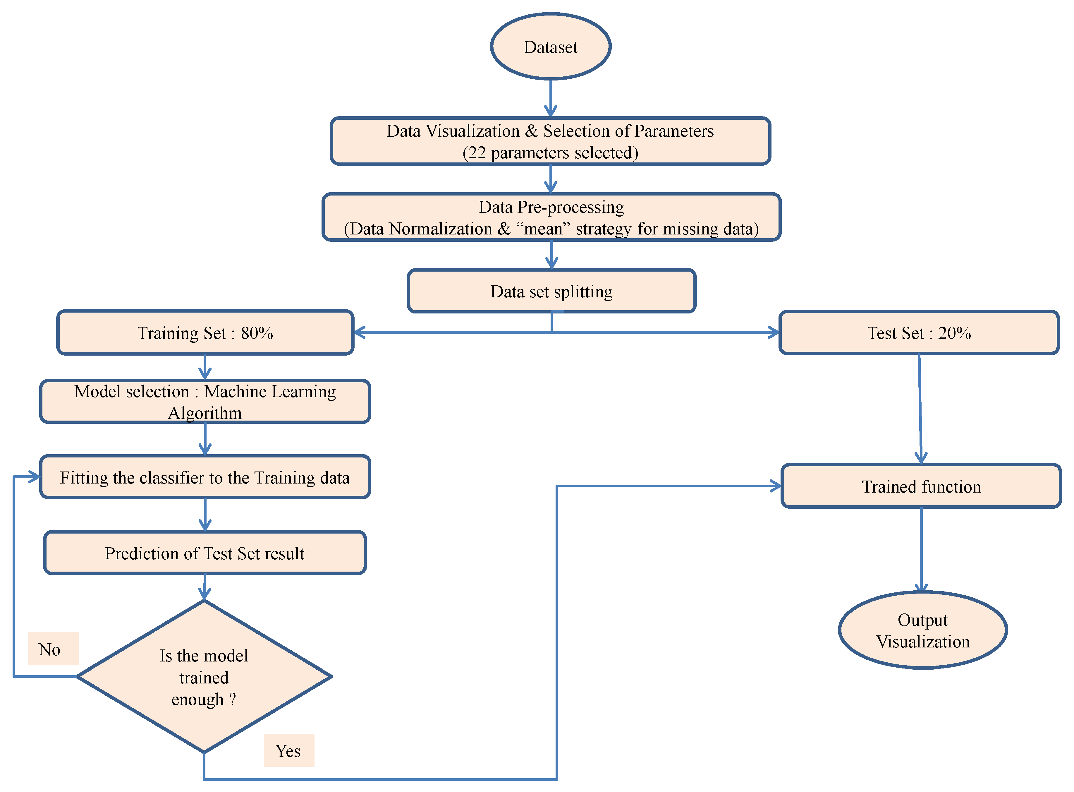
3. ML Modelling Approach

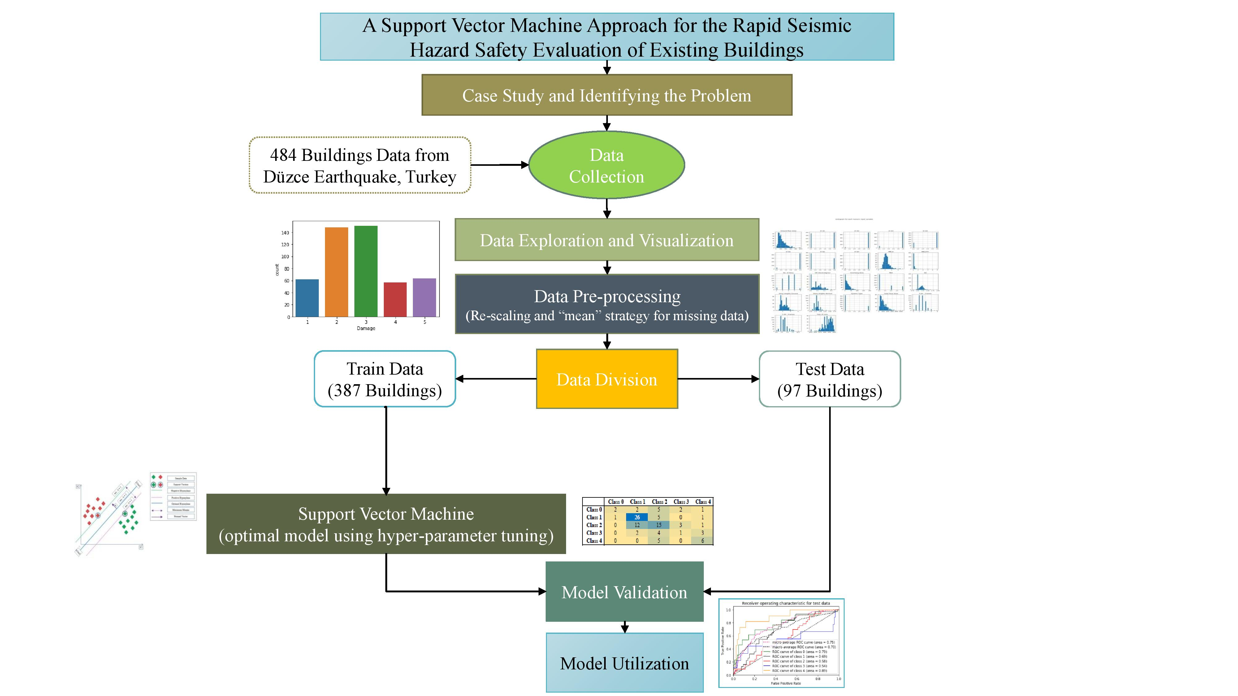
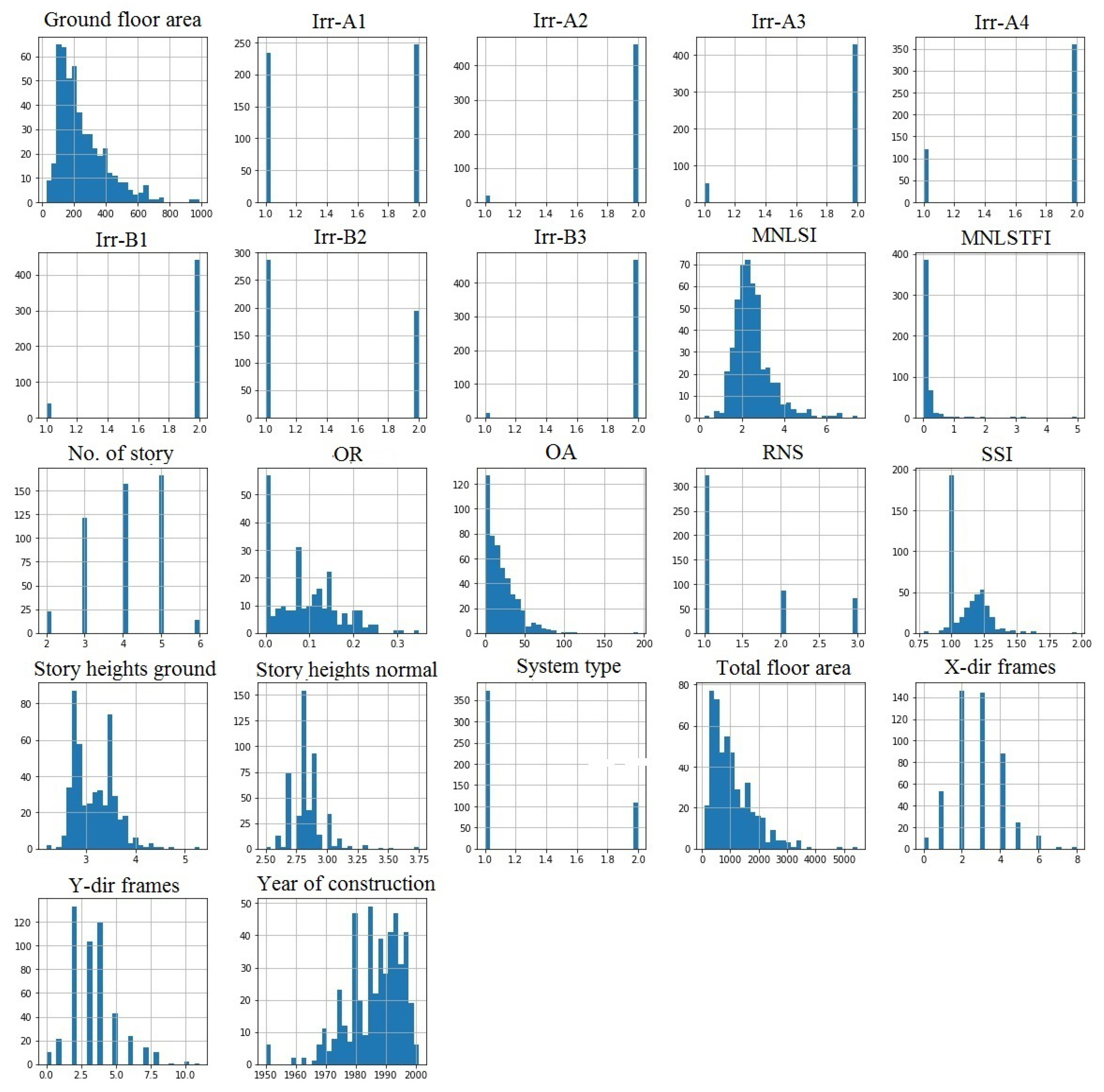
The current segment elaborates on the procedure utilized in predicting the seismic damage vulnerability of the RC buildings post-earthquake, employing the ML technique. ML gains experience while learning through the various pre-defined algorithm, mainly used for classification and regression problems [45]. Figure 1 illustrates the steps for the formulation of the problem, and further levels are found in detail in the following subsections.

3.1. Input Dataset

The first stage for designing the ML model is the selection of input data. The input data here are the independent variables or features points. The ML model classifier explains the effect that features have on the outcome.

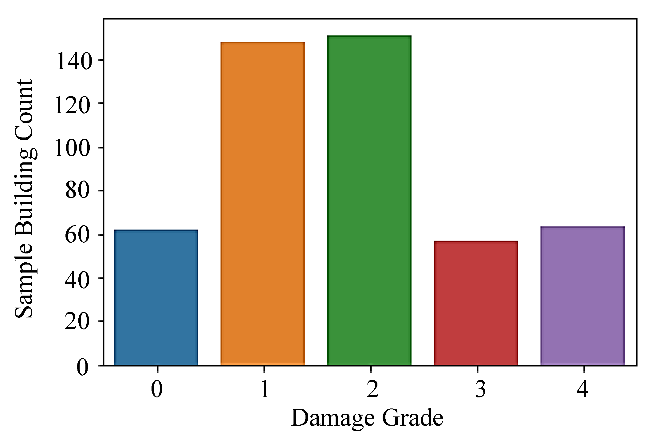
3.2. Classification of Damage Data

SVM is the classification technique that is implemented in this task. The building’s damage class is assigned based on the susceptibility to different damage levels depending on the required purpose.

3.3. Data Pre-Processing

In Statistical data, there are three main data types; numeric, categorical and ordinal. However, ML models can only handle numeric features. To make, the model, work properly, we convert the categorical and ordinal features into numeric features. The conversion of different data forms into numerical is possible by using “Panda” library and creating dummy features, which indicates 1 for the observation that belongs to that category; the other category observations remain as 0. Another option “OneHotEncoder” in “sci-kit learn” library works the same way.

Dataset standardization is a worldwide demand for several ML classifiers enforced in scikit-learn; the performance might not be expected if the individual features do not follow standard normally distributed data. Feature scaling is an alternate option for standardization; it scales the features between an interval of minimum and maximum value, commonly between 0 and 1. It brings the maximum absolute value of each attribute point to a unit size using the classes, such as “MinMaxScaler” or “MaxAbsScaler”. Scaling adds robustness to minimal standard deviations of attributes and perpetuating null entries in the sporadic data.

Another critical aspect to consider is the missing data. However, in the given task, all the data are crucial as they belong to seismic observation. So the alternative solution to replace the missing data is by using the mean, median, or the highest frequency value of the given feature. In case of any missing data in this study, they are filled with the mean value of the features.

3.4. Selection of Input Parameters

ML is capable of computing multi-parametric problems. Based on the area of study, the selection of parameters may differ. For the given task, the selected parameters are the structural parameters characterizing the seismic behavior of the buildings’ posts any earthquake. Structural parameters are observed during the field survey.

3.5. Splitting of Dataset

The ML algorithm uses a recognized dataset segregated into a training subset and a testing subset. The training subset constructs the predictive models, and the testing subset analyses the efficiency of the models. Every data point consists of two attributes: A predictor and its respective classes—the predictors are independent variables with labeled categories. The damage class for each structure is determined by the safety and risk associated with the building. The training subset contains the sample buildings’ damage scale for learning purposes, while the test sub-set keeps the damage scale obscure for accurate prediction of the classifier.

3.6. Model Selection

SVM, as the selected model in this study, was first proposed by Cortes and Vapnik [46]. It belongs to supervised learning and used for classification, regression, and outlier detection. The purpose of the SVM design is to analyze a hyperplane in an N-dimensional feature space that precisely segregates the separate class points. Support vectors are feature points near the hyperplane and impact the hyperplane’s location and arrangement. Support vectors optimize the margin in between the classifier. Hyperplanes act as the choice boundaries which label the feature data. Data points belonging on either side of the hyperplane may associate with distinctive groups. However, the number of feature points decide the dimension of the hyperplane.

SVM is a comparatively new learning algorithm, and the primary difference between SVM and the rest of the ML algorithms is that SVM reduces the viable liability rather than lowering the classification error. This mechanism’s model functioning is to segregate feature points using the hyperplanes to the various classes they belong to, keeping the most significant margin in between classes. A nonlinear mapping transfers the feature points from the primordial space to higher dimensional feature space and drives to search the optimum hyperplane.

Figure 2 shows the mechanism of a linear SVM while classifying different classes. For a two-dimensional space, the middle separator between the two categories is called the discriminator. Therefore, for N-dimensional area, the classifier is a hyperplane. Assuming that the distance between each class data point and the classifier equals to 1 [47].

Let x: Feature vector where $x\in {\mathbb{R}}^n$,

y: Class where $y\in \{1,-1\}$,

w and b: SVM parameters which can be learn using the training set,

$x^{\left(i\right)},y^{\left(i\right)}$: $i^{th}$ sample of the dataset among N sample training set,

then, the class $y\left(i\right)$ for vector $x\left(i\right)$ is determined by:

$$y^{\left(i\right)}=\left\{\begin{array}{cc}-1\hfill & \mathrm{if}{w}^T{x}^{\left(i\right)}+\mathrm{b}\le -1\hfill \\ 1\hfill & \mathrm{if}{w}^T{x}^{\left(i\right)}+\mathrm{b}\ge 1\hfill \end{array}\right.$$

(3)

In order to segregate the classes of data points, many possible hyperplanes are possible. The main objective is to detect a plane that has the maximum margin, i.e., the optimal separation between data points of each class (M). Using Equation (3) the optimal margin (M) is given by:

$$M=\frac{\left(\right|b+1|-|b-1\left|\right)}{\left|\right|w\left|\right|}=\frac{2}{\left|\right|w\left|\right|}.$$

(4)

Furthermore, SVMs are also protracted to solve multi-class problems using the “one-against-one” [48] approach. The same technique is applied to study the task for the damage classification of the buildings with five different damage classes. In ”one-against-one” approach, for n number of classes, there are $n\times \frac{(n-1)}{2}$ classifiers and each one trains data from two classes.

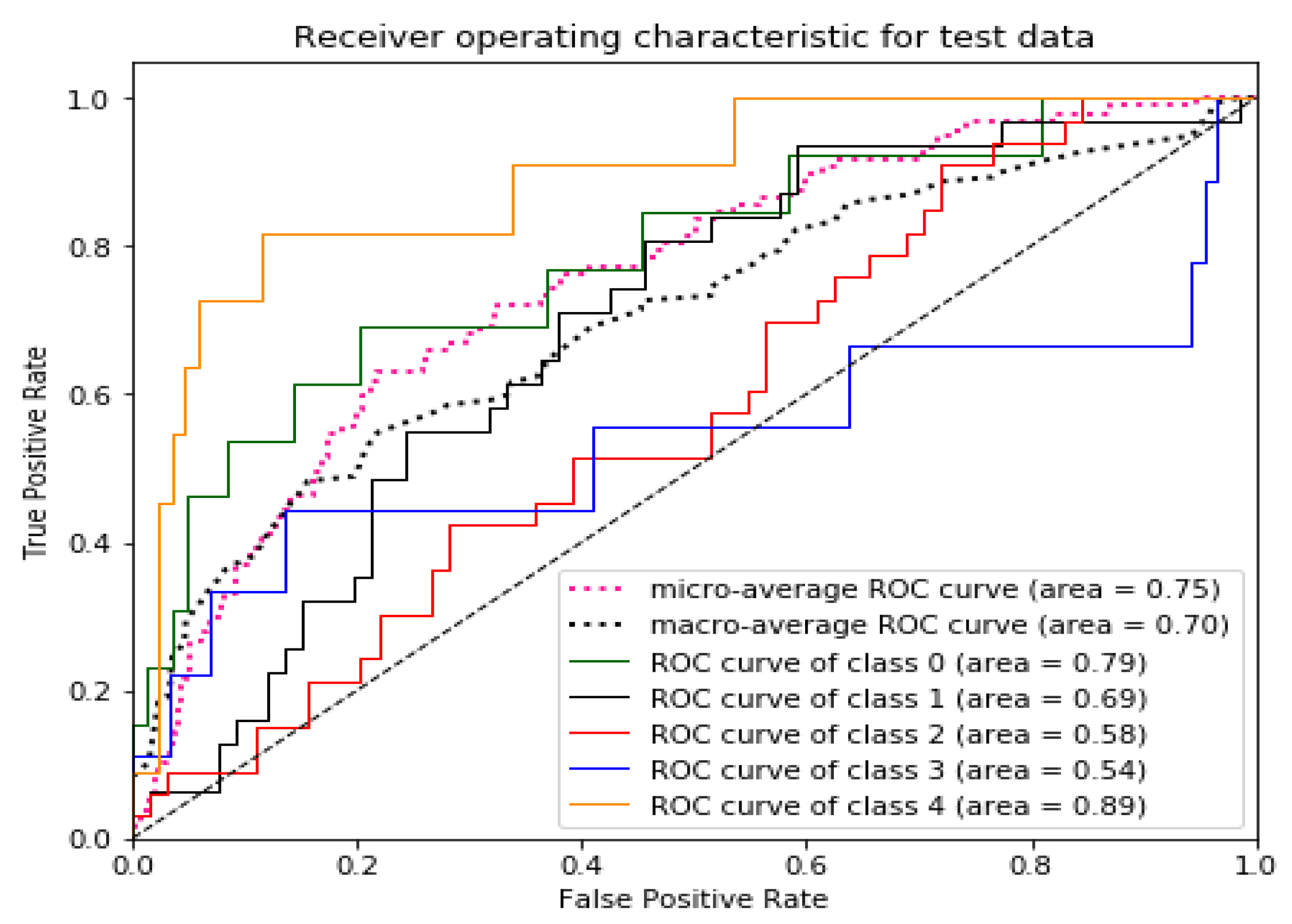
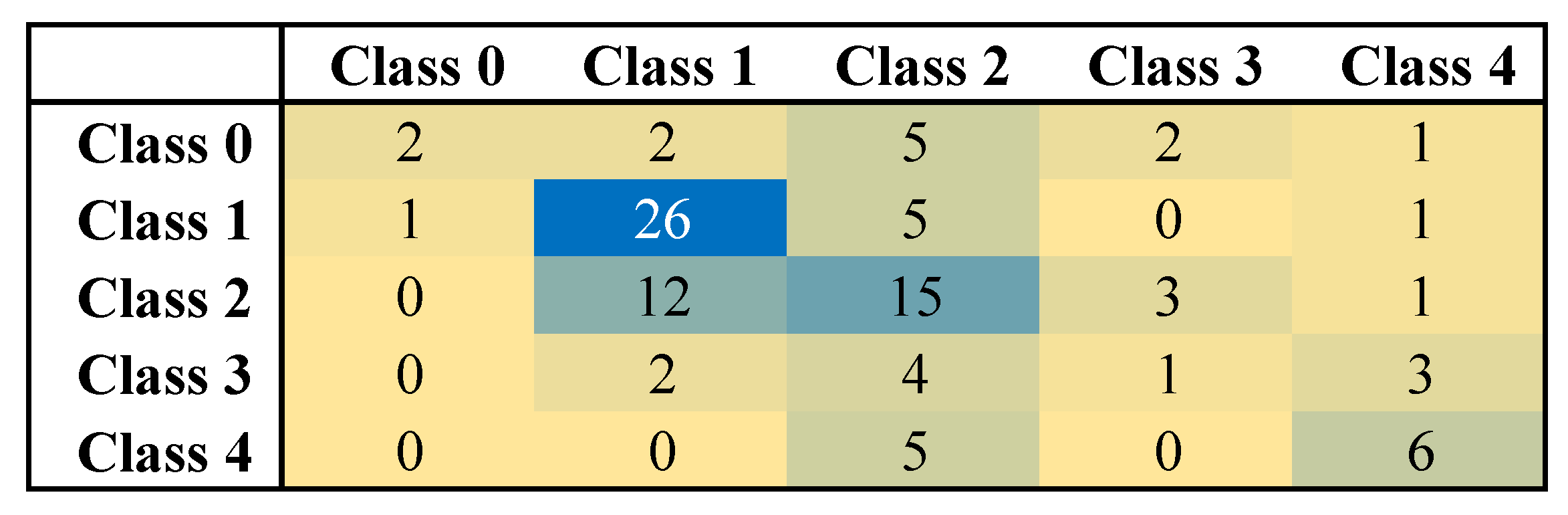
3.7. Evaluating the Performance of Predicted Model

Aim of this section is the evaluation of the classification competence of the created model for the unseen samples in the test subset. For enhancing the model performance, SVM uses several factors like kernel, degree of the kernel function, scaling parameter, and cost of constraints violation (C) as the tunable parameters.

3.8. Model Utilization

The satisfactory model evaluates the unseen examples. The model accuracy depends on many factors, like quantity and quality of input data, selection of features, and the number of outliers. A useful model performs with 50% of overall accuracy for data assessment.

4. Methodology and Database

In this study, the database is collected from the archival material of SERU (Structural Engineering Research Unit) [49]. It was recorded from post-earthquake damage evaluations conducted after the 1999 Düzce earthquake in Turkey and enclosed detailed information on 484 selected buildings deteriorated by various degrees of damage. There are twenty-two feature parameters that the dataset contains such as system type, year of construction, number of stories, ground floor area, total floor area, overhang area, ground story height, normal story height, irregularities in plan and horizontal, X & Y direction frames, MNLSTFI, MNLSI, NRS, SSI, and OR.

Table 1. Characterizing the damage.

Damage State	Damage Grade
None	0
Light	1
Moderate	2
Severe	3
Collapse	4

states the damage grade and the corresponding damage scale used for the risk assessment. Figure 3 shows the distribution of buildings reciprocal to their damage categories. The vulnerability of the RC buildings is measured by anticipating the damage caused post-earthquake.

4.1. Data Pre-Processing

The dataset contained all numeric features, but many of them had missing data points. SimpleImputer class from scikit-learn works well by replacing the missing values using the mean or median values. For the task dataset, the unavailable data points are replaced using “ mean” value. The feature parameter data were standardized in order to proportionate the complete input vector of the dataset to a standard scale, without altering the variance in the ranges of values. Figure 4 shows the distribution of data points over each feature parameter. These parameters as introduced previously are Ground floor area, Irregularities (here as Irr-A1 to Irr-B3), MNLSI, MNLSTFI, No. of story, OR, OA, RNS, SSI, story heights ground and normal, system type, total floor area, frames in X and Y directions, and year of construction. It is clearly observable that the input variables are not distributed ordinarily. The maximum parameter is following Gaussian distribution, like ground floor area, MNLSI, OR, OA, story height ground, total floor area, years of constructions, X-dir frames, Y-dir frames, story height normal, number of story and SSI are following a Gaussian distribution. Whereas different irregularities presented as Irr-A2, Irr-A3, Irr-A4, Irr-B1, Irr-B3 are biased towards the right, and the rests are slanted to the left.

4.2. Splitting of Dataset

As mentioned above, the dataset divides into training and test subset. As a good practice, 80% of the data is for training, and 20% of the data is for test subset. The training set consists of familiar output, and the classifier gains the experience while learning on this data to classify other unseen examples further. The test subset evaluates the predictive performance of the model using its subset.

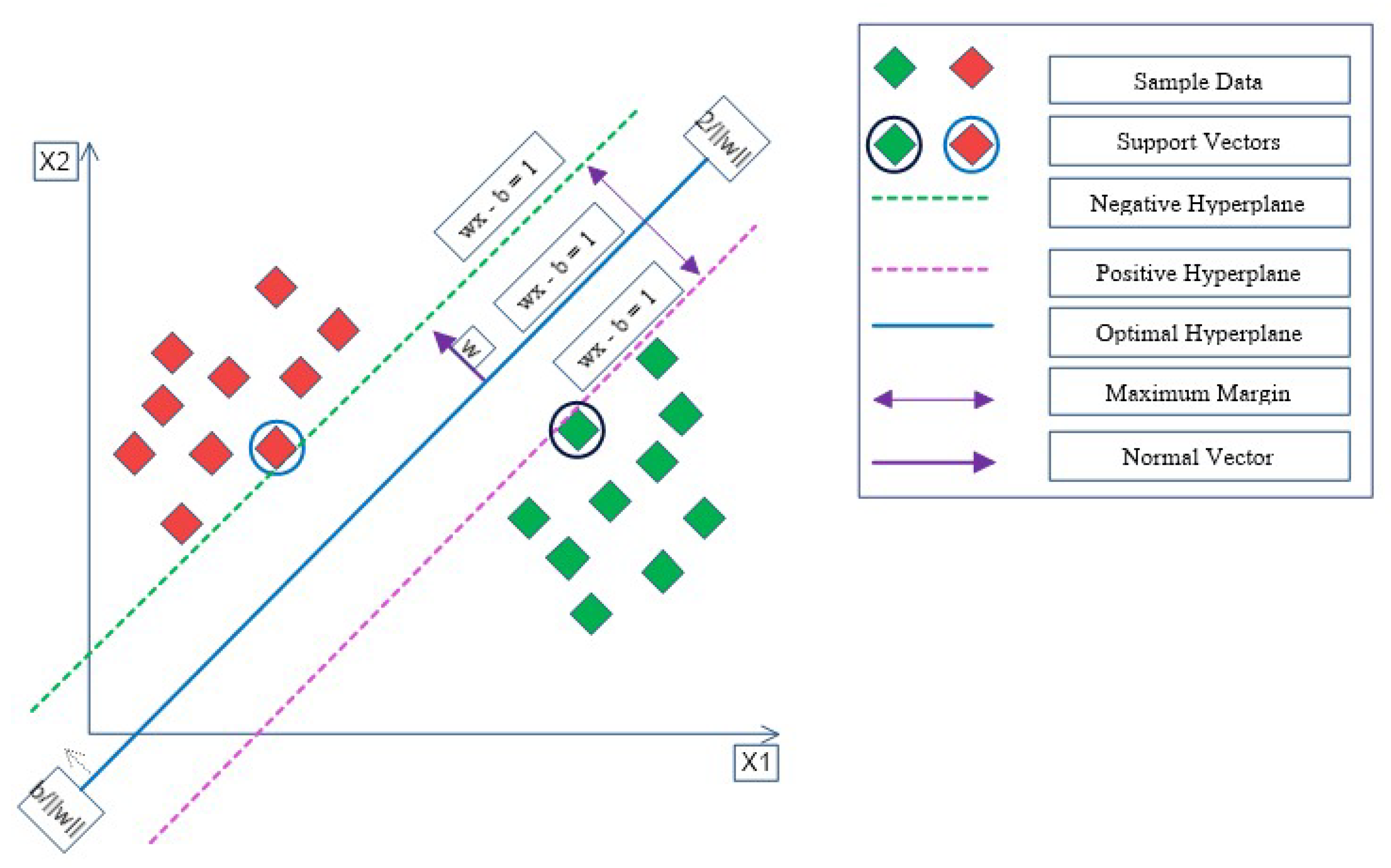
4.3. SVM: Feature Selection and Kernels

Feature selection is important to maximize the performance of the model in terms of accuracy. Tunning certain parameters, model accuracy can be improved. Major parameters include:

• Kernels: Kernels are a combination of mathematical functions. They are designed to collect the input data and alter them into the necessary form. Various SVM mechanisms employ the various form of kernel functions. The kernel functions may vary in types like linear, nonlinear, polynomial, radial basis function (RBF), and sigmoid.
• C (Regularization): C acts as a penalty parameter, which adds an upper bound to the bias of each support vector and manipulates the proximity of fit to the training samples, and kernel value. The misclassification or error term tells the SVM optimization of how much error is bearable. When C is high, it classifies all the data points correctly, but often there is a chance of over-fitting. In counter, when C is low, the optimizer looks for a larger-margin to separate the hyperplane, though the hyperplane misinterprets more points.
• Gamma: Gamma is specific to the RBF kernel, not for the linear or polynomial kernel. The gamma parameter characterizes the effect of a single training sample attainment, where lower gamma means “far”, and higher gamma means “close-by”. Gamma decides the curvature in a decision boundary.

5. Result and Discussion

This task includes the four significant kernels: Polynomial kernel, RBF kernel, Sigmoid kernel, and Linear kernel. The SVM model trains itself using those kernels and generates a predicted output. To train the model optimally and to attain the best possible accuracy, the model is trained ten times using the algorithm, where the highest accuracy is selected out of all the outcomes.

The classifier evaluates each kernel and calculates various values, such as accuracy, precision, and recall.

Table 2. Accuracy of model classifier with different kernels.

Kernel	Accuracy (in %)
RBF	45
Sigmoid	45
Linear	45
Polynomial	26

shows the percentage of accuracy achieved by each kernel. RBF, Sigmoid, and Linear Kernels have identical accuracy of 45%, whereas polynomial performance is lower with an accuracy of 26%.

All the kernels showed an accuracy of less than 50%, which does not make a good model. For accuracy, the model hyper-parameters such as C, gamma, and kernels are tuned. Hyper-parameters do not learn directly; instead, they pass as an argument to the estimator class’s constructor. Grid search in scikit-learn helps to tune the hyper-parameter and to evaluate the SVM model for every combination of algorithm input allocated in the grid. Grid search returns the best estimator, and for this task, the resultant best estimator showed an accuracy of 52% using RBF kernel, whereas the previous study by Tesfamariam [14] in this area of research has accuracy reported 45%.

Figure 5 represents the confusion matrix, which visualizes the performance of the classification model over the test set for which the correct labels are known. Based on the number of classes, the representation is a [5 × 5] matrix. The diagonal numbers in the confusion matrix illustrated the number of occurrences when the model classifier predicted the class correctly. Other numbers across the matrix are misclassified cases. Therefore, higher numbers are desirable in the confusion matrix for an accurate model.

The confusion matrix in the given figure shows that for Class 1, 26 buildings out of 29 RC buildings are classified correctly, and it has the largest value. Class 2 has been poorly classified (15 out of 37).

The performance of the model is also visualized using the Receiver Operating Characteristics (ROC) curve. The ROC curve is a graphical representation of the diagnostic ability of any binary classifier. For the classification of different classes, it breaks down the relationships into all pair-wise comparisons, and the area under the curve is calculated for each lesson match (i.e., lesson O vs. class L; lesson L vs. course M; etc.). The area beneath the curve over the significant pair-wise AUC’s (range under the ROC) shows the variable significance degree. Figure 6 shows the ROC curves for the test data of the classifier. The area under the ROC curve (AUC) shows a descent value, which means the classifier has a good fit with the test set. The micro-average ROC curve area and the macro-average ROC curve area are 0.75 and 0.70, respectively. The graph shows that Class 3 is primarily below the curve, and hence the accuracy of Class 3 is also decreased. Class 0 and Class 1 have attained the optimum value of ROC, meaning the maximum numbers of buildings under these categories are correctly classified.

6. Conclusions

Damage to buildings caused by recent earthquakes clearly shows the need to identify and retrofit vulnerable buildings. However, it is a monumental challenge to strengthen all existing buildings with the required design. However, existing buildings can be classified, representing their associated risk factor. Analyzing the expected damage and its analogous uncertainty is primarily for risk estimation and risk management. The study has considered 22 different features applied as inputs to the method, which include: System type, year of construction, ground floor area, total floor area, overhang area, ground and normal story height, vertical and plan irregularities, X and Y direction frames, number of stories, MNLSTFI, MNLSI, NRS, SSI, and OR. The performance of the model classifier depends on the selection of the input parameter, classification technique, and dataset. A classifier performance will degrade when the feature variable is not sufficient to discriminate the output class criteria explicitly or when outliers and wrong variables are present in the dataset.

The SVM method proposed a good damage classification of the buildings according to their respective damage classes. The technique could be used to help to make strategic risk management decisions and risk assessment for earthquake-prone buildings prior to events. The results showed an accuracy of 52% when using all 22 parameters, which is an acceptable rate for the sample size used. In the future, the model accuracy should be improved by training the model with the most useful parameters. In addition, using the k-fold cross-validation technique is advised to verify the performance of the model classifier.

References

1. Jain, S.; Mitra, K.; Kumar, M.; Shah, M. A proposed rapid visual screening procedure for seismic evaluation of RC-frame buildings in India. Earthq. Spectra 2010, 26. [Google Scholar] [CrossRef]
2. Chanu, N.; Nanda, R. A Proposed Rapid Visual Screening Procedure for Developing Countries. Int. J. Geotech. Earthq. Eng. 2018, 9, 38–45. [Google Scholar] [CrossRef]
3. Sinha, R.; Goyal, A.A. A national policy for seismic vulnerability assessment of buildings and procedure for rapid visual screening of buildings for potential seismic vulnerability. In Report to Disaster Management Division; Ministry of Home Affairs, Government of India: New Delhi, India, 2004. [Google Scholar]
4. Rapid Visual Screening of Buildings for Potential Seismic Hazards: A Handbook, 3rd ed.; FEMA P-154; Homeland Security Dept, Federal Emergency Management Agency: Washington, DC, USA, 2015.
5. Harirchian, E.; Lahmer, T.; Buddhiraju, S.; Mohammad, K.; Mosavi, A. Earthquake Safety Assessment of Buildings through Rapid Visual Screening. Buildings 2020, 10, 51. [Google Scholar] [CrossRef] [Green Version]
6. Rai, D.C. Seismic Evaluation and Strengthening of Existing Buildings; IIT Kanpur and Gujarat State Disaster Mitigation Authority: Gandhinagar, India, 2005; pp. 1–120. [Google Scholar]
7. Vallejo, C.B. Rapid Visual Screening of Buildings in the City of Manila, Philippines. In Proceedings of the 5th Civil Engineering Conference in the Asian Region and Australasian Structural Engineering Conference 2010; Engineers Australia: Sydney, Australia, 2010; pp. 513–518. [Google Scholar]
8. Mishra, S. Guide Book for Integrated Rapid Visual Screening of Buildings for Seismic Hazard; TARU Leading Edge Private Ltd.: Guragon, India, 2014. [Google Scholar]
9. Luca, F.; Verderame, G. Seismic Vulnerability Assessment: Reinforced Concrete Structures; Springer: Berlin/Heidelberg, Germany, 2015; pp. 1–31. [Google Scholar] [CrossRef]
10. Chanu, N.; Nanda, R. Rapid Visual Screening Procedure of Existing Building Based on Statistical Analysis. Int. J. Disast. Risk Reduc. 2018, 28. [Google Scholar] [CrossRef]
11. Özhendekci, N.; Özhendekci, D. Rapid Seismic Vulnerability Assessment of Low- to Mid-Rise Reinforced Concrete Buildings Using Bingöl’s Regional Data. Earthq. Spectra 2012, 28, 1165–1187. [Google Scholar] [CrossRef]
12. Harirchian, E.; Lahmer, T.; Rasulzade, S. Earthquake Hazard Safety Assessment of Existing Buildings Using Optimized Multi-Layer Perceptron Neural Network. Energies 2020, 13, 2060. [Google Scholar] [CrossRef] [Green Version]
13. Arslan, M.; Ceylan, M.; Koyuncu, T. An ANN approaches on estimating earthquake performances of existing RC buildings. Neural Netw. World 2012, 22, 443–458. [Google Scholar] [CrossRef] [Green Version]
14. Tesfamariam, S.; Liu, Z. Earthquake induced damage classification for reinforced concrete buildings. Struct. Saf. 2010, 32, 154–164. [Google Scholar] [CrossRef]
15. Harirchian, E.; Harirchian, A. Earthquake Hazard Safety Assessment of Buildings via Smartphone App: An Introduction to the Prototype Features- 30. Forum Bauinformatik: von jungen Forschenden für junge Forschende: September 2018, Informatik im Bauwesen; Professur Informatik im Bauwesen, Bauhaus-Universität Weimar: Weimar, Germany, 2018; pp. 289–297. [Google Scholar] [CrossRef]
16. Ketsap, A.; Hansapinyo, C.; Kronprasert, N.; Limkatanyu, S. Uncertainty and fuzzy decisions in earthquake risk evaluation of buildings. Eng. J. 2019, 23, 89–105. [Google Scholar] [CrossRef]
17. Mandas, A.; Dritsos, S. Vulnerability assessment of RC structures using fuzzy logic. WIT Trans. Ecol. Environ. 2004, 77. [Google Scholar] [CrossRef]
18. Tesfamariam, S.; Saatcioglu, M. Seismic vulnerability assessment of reinforced concrete buildings using hierarchical fuzzy rule base modeling. Earthq. Spectra 2010, 26, 235–256. [Google Scholar] [CrossRef]
19. Şen, Z. Rapid visual earthquake hazard evaluation of existing buildings by fuzzy logic modeling. Expert Syst. Appl. 2010, 37, 5653–5660. [Google Scholar] [CrossRef]
20. Harirchian, E.; Lahmer, T. Improved Rapid Visual Earthquake Hazard Safety Evaluation of Existing Buildings Using a Type-2 Fuzzy Logic Model. Appl. Sci. 2020, 10, 2375. [Google Scholar] [CrossRef] [Green Version]
21. Cerovecki, A.; Gharahjeh, S.; Harirchian, E.; Ilin, D.; Okhotnikova, K.; Kersten, J. Evaluation of Change Detection Techniques using Very High Resolution Optical Satellite Imagery. In Preface 2 Summer Course 2015; Bauhaus-Universitätsverlag: Weimar, Germany, 2018; p. 20. [Google Scholar]
22. Ezquerro, P.; Del Soldato, M.; Solari, L.; Tomás, R.; Raspini, F.; Ceccatelli, M.; Fernández-Merodo, J.A.; Casagli, N.; Herrera, G. Vulnerability Assessment of Buildings due to Land Subsidence Using InSAR Data in the Ancient Historical City of Pistoia (Italy). Sensors 2020, 20, 2749. [Google Scholar] [CrossRef]
23. Harirchian, E. Constructability Comparison between IBS and Conventional Construction. Ph.D. Thesis, Universiti Teknologi Malaysia, Kuala Lumpur, Malaysia, 2015. [Google Scholar]
24. Kegyes-Brassai, O. Vulnerability Assessment of Buildings Based on Rapid Visual Screening and Pushover: Case Study of Gyor, Hungary. In Computational Methods and Experimental Measurements XIX & Earthquake Resistant Engineering Structures XII; WIT Press: Southampton, UK, 2019; Volume 185, pp. 63–74. [Google Scholar] [CrossRef]
25. Morfidis, K.; Kostinakis, K. Seismic parameters’ combinations for the optimum prediction of the damage state of R/C buildings using neural networks. Adv. Eng. Softw. 2017, 106, 1–16. [Google Scholar] [CrossRef]
26. Sucuoglu, H.; Yazgan, U.; Yakut, A. A Screening Procedure for Seismic Risk Assessment in Urban Building Stocks. Earthq. Spectra 2007, 23. [Google Scholar] [CrossRef]
27. Aldemir, A.; Sahmaran, M. Rapid screening method for the determination of seismic vulnerability assessment of RC building stocks. Bull. Earthq. Eng. 2019. [Google Scholar] [CrossRef]
28. Askan, A.; Yucemen, M. Probabilistic methods for the estimation of potential seismic damage: Application to reinforced concrete buildings in Turkey. Struct. Saf. 2010, 32, 262–271. [Google Scholar] [CrossRef]
29. Morfidis, K.; Kostinakis, K. Use of Artificial Neural Networks in the R/C Buildings’ Seismic Vulnerabilty Assessment: The Practical Point of View. In Proceedings of the 7th ECCOMAS Thematic Conference on Computational Methods in Structural Dynamics and Earthquake Engineering, Crete, Greece, 24–26 June 2019; Aristotle University of Thessaloniki: Thessaloniki, Greece, 2019; Volume 18969, No. IKEECONF-2019-411. pp. 5435–5455. [Google Scholar] [CrossRef] [Green Version]
30. Dritsos, S.; Moseley, V. A fuzzy logic rapid visual screening procedure to identify buildings at seismic risk. Beton- und Stahlbetonbau 2013, 136–143. Available online: https://www.researchgate.net/publication/295594396_A_fuzzy_logic_rapid_visual_screening_procedure_to_identify_buildings_at_seismic_risk (accessed on 30 June 2020).
31. Zhang, Z.; Hsu, T.Y.; Wei, H.H.; Chen, J.H. Development of a Data-Mining Technique for Regional-Scale Evaluation of Building Seismic Vulnerability. Appl. Sci. 2019, 9, 1502. [Google Scholar] [CrossRef] [Green Version]
32. Stone, H. Exposure and Vulnerability for Seismic Risk Evaluations. Ph.D. Thesis, UCL (University College London), London, UK, 2018. [Google Scholar]
33. Harirchian, E.; Lahmer, T. Earthquake Hazard Safety Assessment of Buildings via Smartphone App: A Comparative Study. IOP Conf. Ser. Mater. Sci. Eng. 2019, 652, 012069. [Google Scholar] [CrossRef]
34. Yakut, A.; Aydogan, V.; Ozcebe, G.; Yucemen, M. Preliminary Seismic Vulnerability Assessment of Existing Reinforced Concrete Buildings in Turkey. In Seismic Assessment and Rehabilitation of Existing Buildings; Springer: Berlin/Heidelberg, Germany, 2003; pp. 43–58. [Google Scholar]
35. Yücemen, M.; Özcebe, G.; Pay, A. Prediction of potential damage due to severe earthquakes. Struct. Saf. 2004, 26, 349–366. [Google Scholar] [CrossRef]
36. Yakut, A.; Ozcebe, G.; Yucemen, M.S. Seismic vulnerability assessment using regional empirical data. Earthq. Eng. Struct. Dyn. 2006, 35, 1187–1202. [Google Scholar] [CrossRef]
37. Achs, G.; Adam, C. A Rapid-Visual-Screening Methodology for the Seismic Vulnerability Assessment of Historic Brick-Masonry Buildings in Vienna. In Proceedings of the 15th World Conference on Earthquake Engineering (15 WCEE), Lisbon, Portugal, 24–28 September 2012; pp. 1833–1856. [Google Scholar]
38. Yakut, A. Reinforced Concrete Frame Construction; Summary Publication; Middle East Technical University: Ankara, Turkey, 2004; pp. 1–9. [Google Scholar]
39. Kathir. Construction of Reinforced Concrete Shear Walls, Civil Snapshot. Available online: https://civilsnapshot.com/shear-wall/ (accessed on 20 December 2019).
40. Yakut, A.; Ozcebe, G.; Yucemen, M.S. A statistical procedure for the assessment of seismic performance of existing reinforced concrete buildings in Turkey. In Proceedings of the 13th World Conference on Earthquake Engineering, Vancouver, BC, Canada, 1–6 August 2004; Volume 13. [Google Scholar]
41. Law Insider. Available online: https://www.lawinsider.com/dictionary/ground-floor-area (accessed on 10 February 2020).
42. Tesfamariam, S.; Saatcioglu, M. Risk-based seismic evaluation of reinforced concrete buildings. Earthq. Spectra 2008, 24, 795–821. [Google Scholar] [CrossRef]
43. Ozcebe, G.; Sucuoglu, H.; Yucemen, M.S.; Yakut, A.; Kubin, J. Seismic Risk Assessment of Existing Building Stock in Istanbul a Pilot Application in Zeytinburnu District. In Proceedings of the 8th US National Conference on Earthquake Engineering, San Fransisco, CA, USA, 18–22 April 2006. [Google Scholar]
44. Wasti, S.T.; Özcebe, G. Seismic Assessment and Rehabilitation of Existing Buildings; Springer Science & Business Media: Dordrecht, The Netherlands, 2003; Volume 29, pp. 31–34. [Google Scholar] [CrossRef]
45. Mitchell, T.M. Machine Learning; McGraw Hill: Burr Ridge, IL, USA, 1997; Volume 45, pp. 870–877. [Google Scholar]
46. Cortes, C.; Vapnik, V.N. Support Vector Networks. Mach. Learn. 1995, 20, 273–295. [Google Scholar] [CrossRef]
47. Kia, A.; Sensoy, S. Classification of earthquake-induced damage for R/C slab column frames using multiclass SVM and its combination with MLP neural network. Math. Probl. Eng. 2014, 2014, 734072. [Google Scholar] [CrossRef]
48. Knerr, S.; Personnaz, L.; Dreyfus, G. Single-layer learning revisited: A stepwise procedure for building and training a neural network. In Neurocomputing; Springer: Berlin/Heidelberg, Germany, 1990; Volume 68, pp. 41–50. [Google Scholar]
49. SERU. Middle East Technical University, Ankara, Turkey. Archival Material from Düzce Database Located at Website. Available online: http://www.seru.metu.edu.tr (accessed on 19 April 2020).
Figure 1. Flow chart for ML methodology implementation.
Energies 13 03340 g001
Figure 2. Optimal hyperplane using the SVM algorithm.
Energies 13 03340 g002
Figure 3. Number of buildings as per the damage grade.
Energies 13 03340 g003
Figure 4. Distribution of data on each input variable.
Energies 13 03340 g004
Figure 5. Confusion matrix.
Energies 13 03340 g005
Figure 6. ROC curves for each class of test dataset.
Energies 13 03340 g006