
A Harmonic Compensation Method Using a Lock-In Amplifier under Non-Sinusoidal Grid Conditions for Single Phase Grid Connected Inverters †


Abstract
1. Introduction
1.1. Motivation
1.2. Literature
- (1)
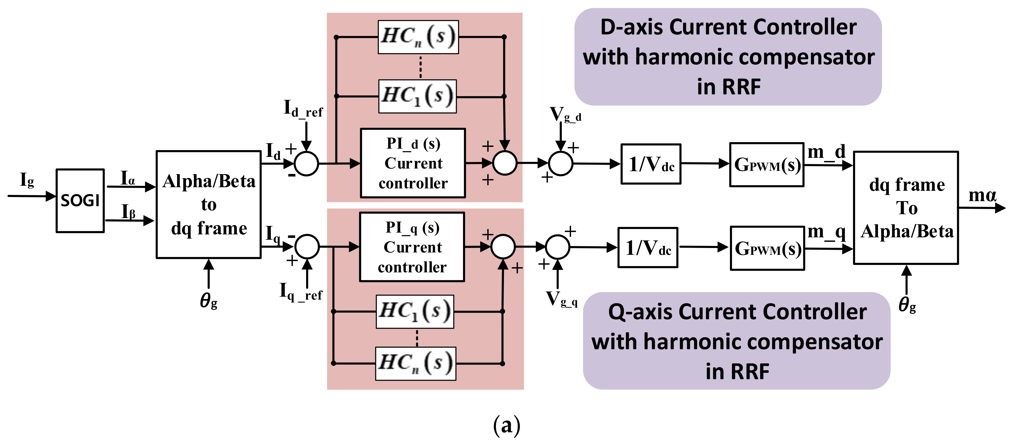
- This method requires two compensators for each D and Q axis to eliminate a certain harmonic. Since a harmonic component in the SRF appears as two different frequency components in the RRF, it should be compensated for both the D and Q axis [32].
- (2)
- Another disadvantage is that the orthogonal signals are generated by the SOGI, which is composed of a low pass filter (LPF) and a band pass filter (BPF). As a result, it attenuates the harmonic information due to filtering, which makes it impossible to extract accurate information about the harmonic component. Thus, the harmonic compensator is not able to perfectly compensate the harmonic.
- (1)
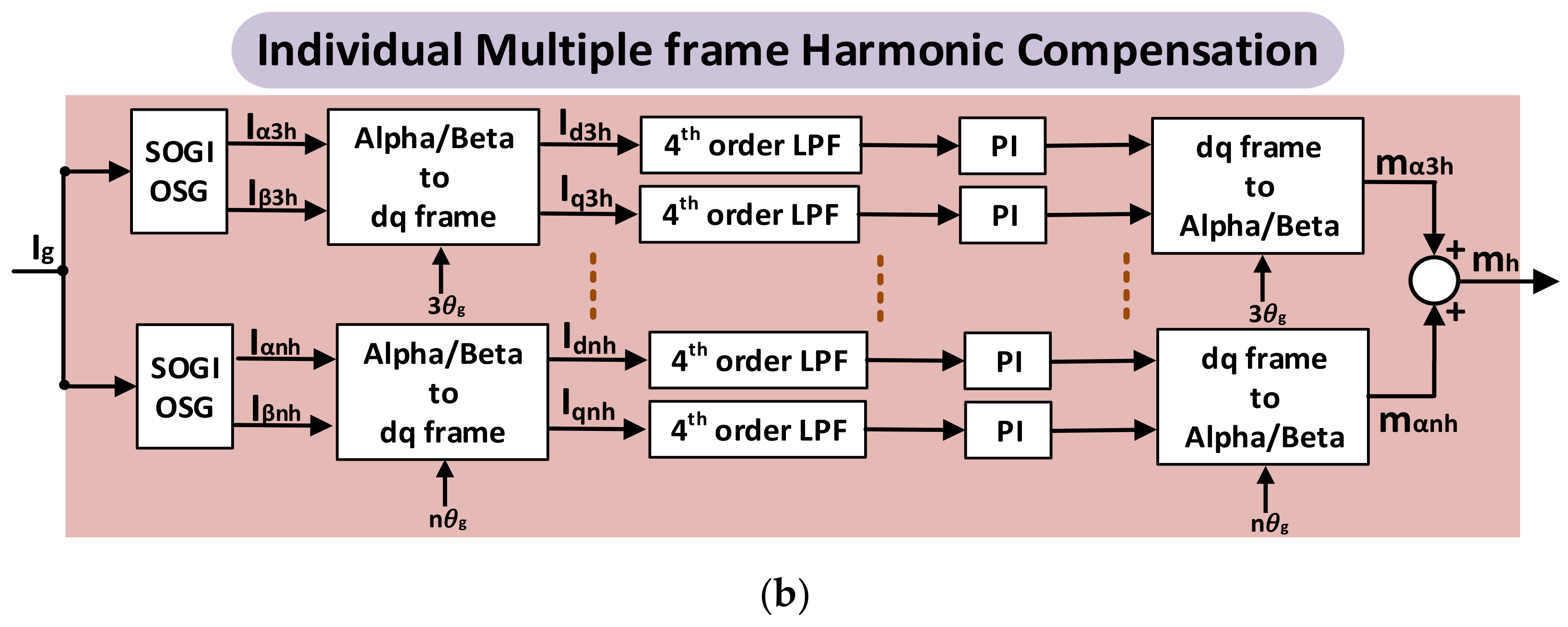
- The computational burden is high, and its dynamic characteristics are not good enough due to the delay produced by the OSG block, high order LPF for multiple numbers of RRFs, and the transformations required to transform AC components into DC components and vice versa.
- (2)
- (3)
- Furthermore, the OSG may generate asymmetric signals, which degrades the performance of the harmonic compensator (PI controller).
- (4)
- In addition, when a SOGI is used to generate the orthogonal signals, it attenuates the harmonic information due to filtering, which makes it difficult to perfectly eliminate the harmonic.
1.3. Advancement
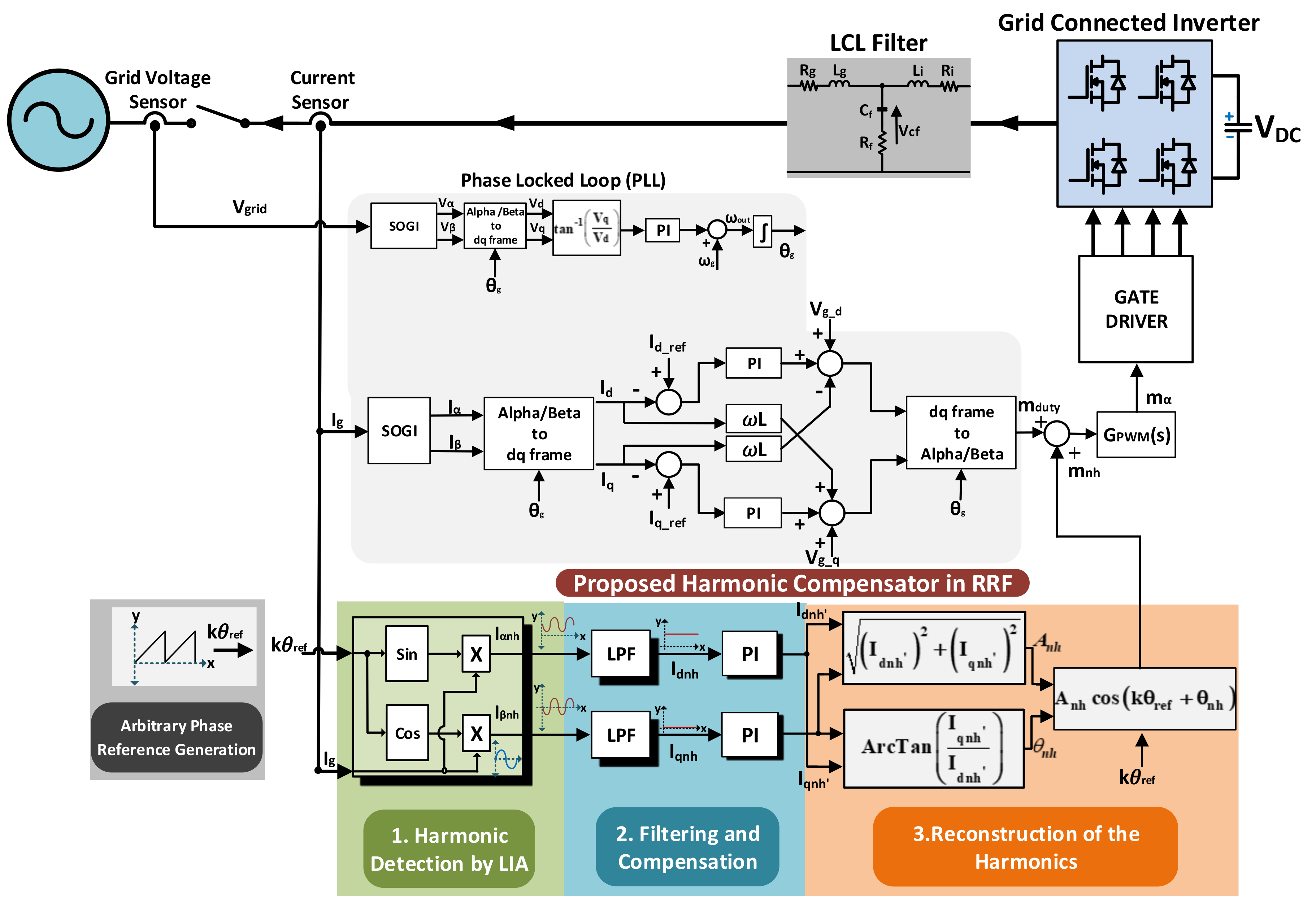
- (1)
- The LIA can extract the amplitude and the phase of a harmonic with a high accuracy, which results in a more effective harmonic compensation than those obtained with conventional methods.
- (2)
- The harmonic detection is performed by using a reference signal with an arbitrary theta, which is independent of the grid theta detected by the PLL, eliminating the concerns of using a grid theta that is polluted by distorted grid conditions, such as grid harmonics, DC offset, etc.
- (3)
- The OSG is not required for harmonic compensation, which eliminates the concerns about the asymmetric generation of orthogonal signals and attenuation of harmonic information.
- (4)
- The transformations from SRF to RRF and from RRF to SRF for harmonic detection are not required.
- (5)
- In the proposed LIA harmonic compensation, the LPF used to eliminate the AC ripples and the PI harmonic compensator both are designed the same for the nth harmonic order. Thus, it will reduce the design complexity and less effort will be applied for better performance of the system.
2. Proposed Lock-In Amplifier (LIA) Harmonic Compensation Method
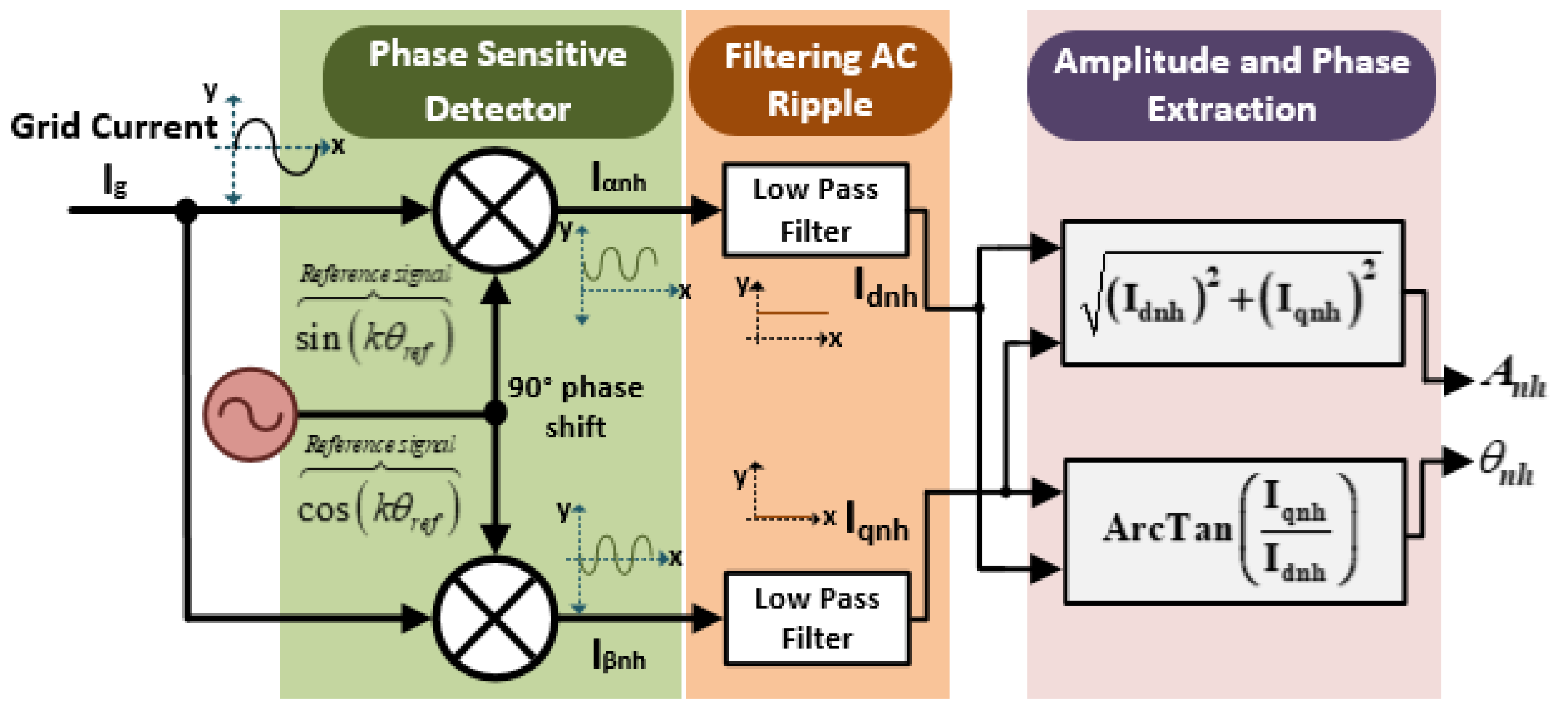
- (1)
- Through the PSD, all of the input signals where the frequencies are not the same as the reference signal are rejected and only an input signal with the same frequency as the reference signal is converted to a zero-frequency component, i.e., a DC quantity.
- (2)
- The other frequencies present in the input signals are converted into two AC signals, one is at the difference of frequency, and the other is at the sum of frequency due to frequency shifting property of PSD.
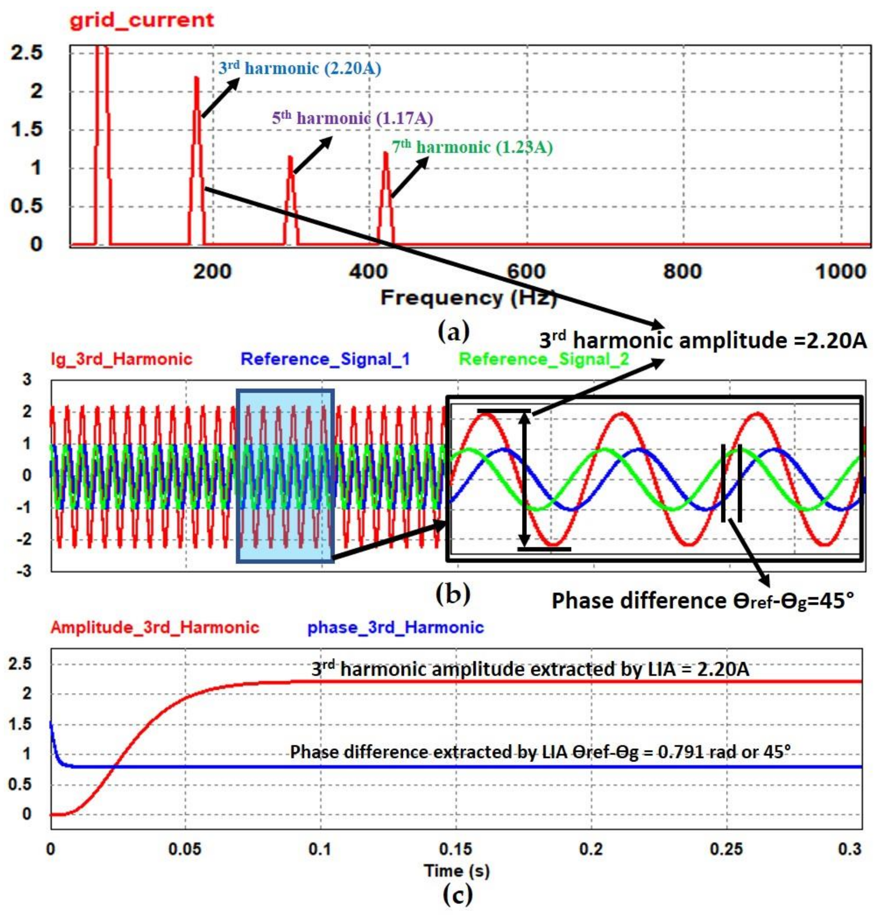
2.1. Detection of Harmonics Using Lock-In Amplifier
2.2. Filtering AC Ripple
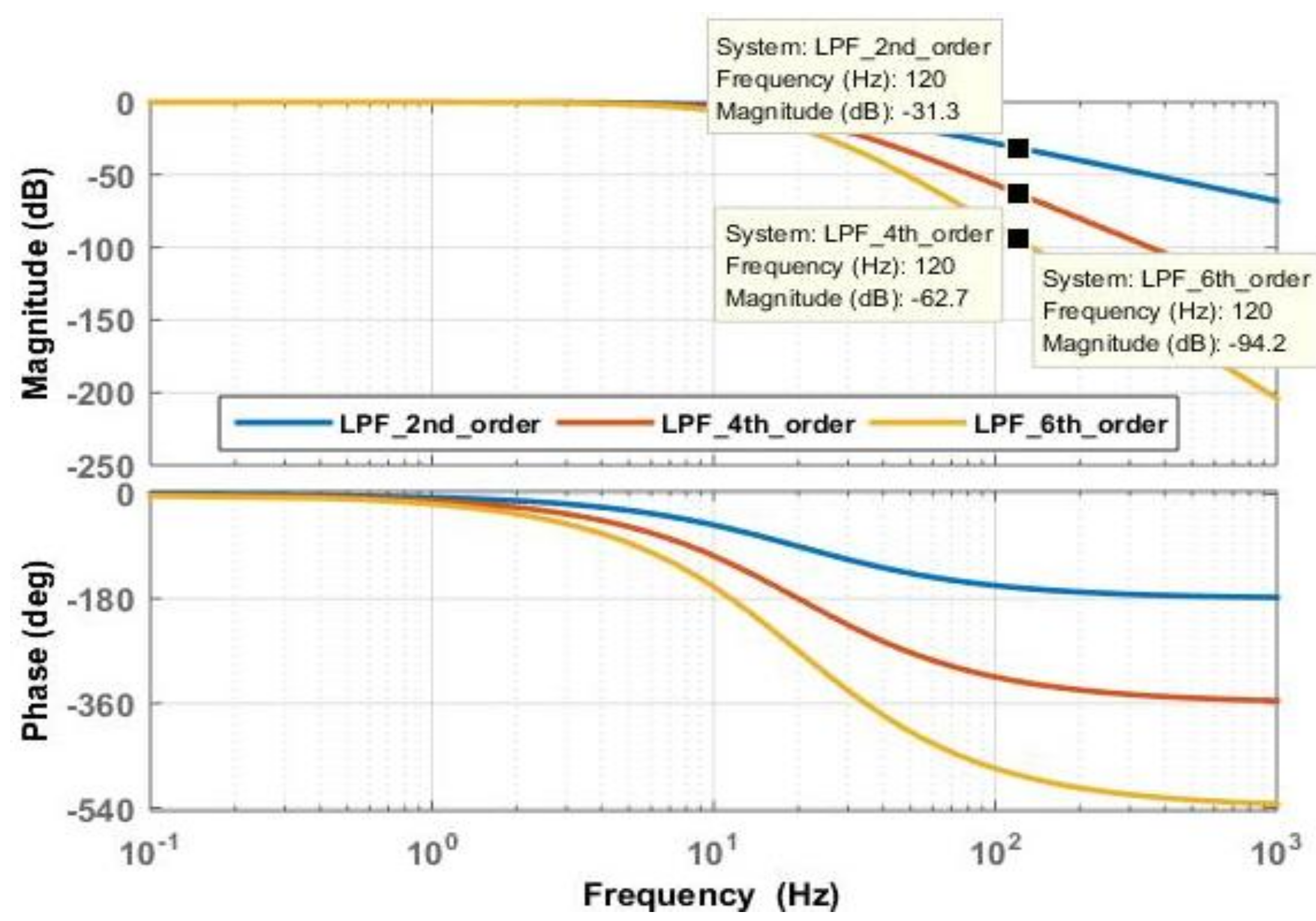
Low Pass Filter Design Criteria
2.3. Reconstruction of the Harmonic
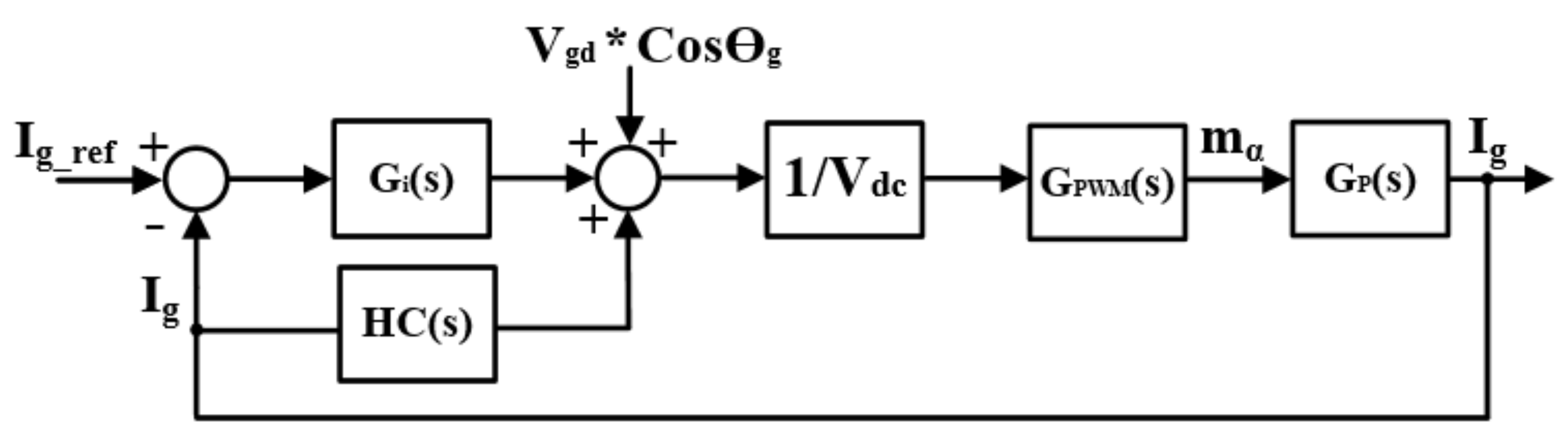
3. Controller Design Considerations of the Propose Method
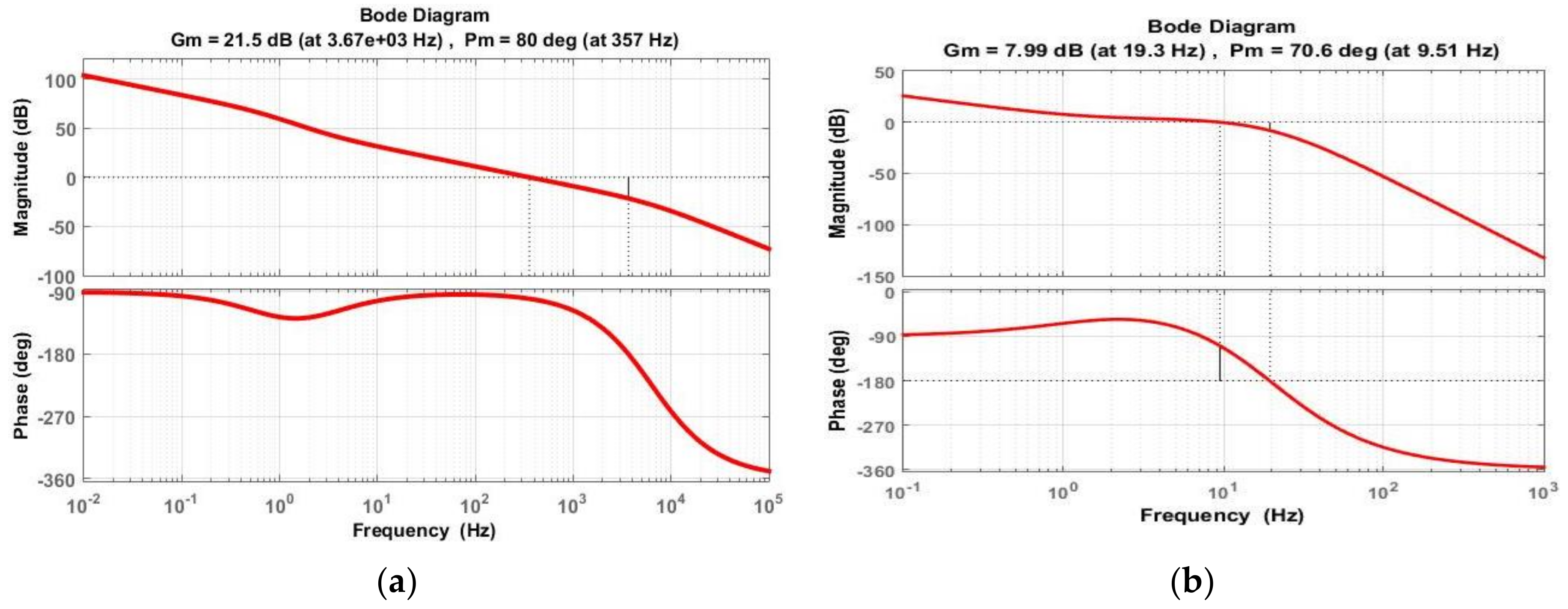
3.1. Design of the Fundamental Current Controller
3.2. Design of the Harmonic Compensator
4. Simulation Results
5. Experimental Results
6. Conclusions
Author Contributions
Funding
Institutional Review Board Statement
Informed Consent Statement
Data Availability Statement
Conflicts of Interest
References
- Sinsukthavorn, W.; Ortjohann, E.; Mohd, A.; Hamsic, N.; Morton, D. Control strategy for three-/four-wire-inverter-based distributed generation. IEEE Trans. Ind. Electron. 2012, 59, 3890–3899. [Google Scholar] [CrossRef]
- Trujillo, C.; Velasco, D.; Garcera, G.; Figueres, E.; Guacaneme, J. Reconfigurable control scheme for a PV micro inverter working in both grid-connected and island modes. IEEE Trans. Ind. Electron. 2013, 60, 1582–1595. [Google Scholar] [CrossRef]
- Branco, C.G.C.; Torrico-Bascope, R.P.; Cruz, C.M.T.; de Lima, F.K.A. Proposal of three-phase high-frequency transformer isolation UPS topologies for distributed generation applications. IEEE Trans. Ind. Electron. 2013, 60, 1520–1531. [Google Scholar] [CrossRef]
- Wai, R.J.; Lin, C.Y.; Huang, Y.C.; Chang, Y.R. Design of high-performance stand-alone and grid-connected inverter for distributed generation applications. IEEE Trans. Ind. Electron. 2013, 60, 1542–1555. [Google Scholar] [CrossRef]
- Kjaer, S.B.; Pedersen, J.K.; Blaabjerg, F. A review of single-phase grid-connected inverters for photovoltaic modules. IEEE Trans. Ind. Appl. 2005, 41, 1292–1306. [Google Scholar] [CrossRef]
- IEEE Standard for Interconnecting Distributed Resources with Electric Power Systems; IEEE15471; IEEE: Piscataway, NJ, USA, 2005.
- IEEE Recommended Practices and Requirements for Harmonic Control in Electrical Power Systems; IEEE Standard 519-1992; IEEE: Piscataway, NJ, USA, 1992.
- He, G.; Xu, D.; Chen, M. A novel control strategy of suppressing DC current injection to the grid for single-phase PV inverter. IEEE Trans. Power Electron. 2015, 30, 1266–1274. [Google Scholar] [CrossRef]
- Wang, X.; Ruan, X.; Liu, S.; Tse, C.K. Full Feedforward of Grid Voltage for Grid-Connected Inverter with LCL Filter to Suppress Current Distortion Due to Grid Voltage Harmonics. IEEE Trans. Power Electron. 2010, 23, 3119–3127. [Google Scholar] [CrossRef]
- Hong, L.; Tian, Y.; Zhang, J.; Li, D.; Xu, D.; Chen, G. High precision compensation for high power Hybrid Active Power Filter based on repetitive control algorithm. In Proceedings of the 2011 IEEE International Symposium on Industrial Electronics, Gdansk, Poland, 27–30 June 2011; pp. 295–300. [Google Scholar]
- Mohamed, Y.A.R.I.; El-Saadany, E.F. A Control Scheme for PWM Voltage-Source Distributed-Generation Inverters for Fast Load Voltage Regulation and Effective Mitigation of Unbalanced Voltage Disturbances. IEEE Trans. Ind. Electron. 2008, 55, 2072–2084. [Google Scholar] [CrossRef]
- Zhang, X.; Wang, Y.; Yu, C.; Guo, L.; Cao, R. Hysteresis Model Predictive Control for High-Power Grid-Connected Inverters with Output LCL Filter. IEEE Trans. Ind. Electron. 2016, 63, 246–256. [Google Scholar] [CrossRef]
- Timbus, A.; Liserre, M.; Teodorescu, R.; Rodriguez, P.; Blaabjerg, F. Evaluation of current controllers for distributed power generation systems. IEEE Trans. Power Electron. 2009, 24, 654–664. [Google Scholar] [CrossRef]
- Castilla, M.; Miret, J.; Camacho, A.; Matas, J.; de Vicuna, L.G. Reduction of Current Harmonic Distortion in Three-Phase Grid Connected Photovoltaic Inverters via Resonant Current Control. IEEE Trans. Ind. Electron. 2013, 60, 1464–1472. [Google Scholar] [CrossRef]
- Trinh, Q.N.; Lee, H.H. An Enhanced Grid Current Compensator for Grid-Connected Distributed Generation Under Nonlinear Loads and Grid Voltage Distortions. IEEE Trans. Ind. Electron. 2014, 61, 6528–6537. [Google Scholar] [CrossRef]
- Liserre, M.; Blaabjerg, F.; Hansen, S. Design and control of an LCL-filter-based hree-phase active rectifier. IEEE Trans. Ind. Appl. 2005, 41, 1281–1291. [Google Scholar] [CrossRef]
- Twining, E.; Holmes, D.G. Grid current regulation of a three-phase voltage source inverter with an LCL input filter. IEEE Trans. Power. Electron. 2003, 18, 888–895. [Google Scholar] [CrossRef]
- Kazmierkowski, M.P.; Malesani, L. Current control techniques for three-phase voltage-source PWM converters: A survey. IEEE Trans. Ind. Electron. 1998, 45, 691–703. [Google Scholar] [CrossRef]
- Ebrahimi, M.; Khajehoddin, S.A.; Ghartemani, M.K. Fast and Robust Single-Phase DQ Current Controller for Smart Inverter Applications. IEEE Trans. Power Electron. 2016, 31, 3968–3976. [Google Scholar] [CrossRef]
- Ciobotaru, M.; Teodorescu, R.; Blaabjerg, F. A new single-phase PLL structure based on second order generalized integrator. In Proceedings of the 37th IEEE Power Electronics Specialists Conference, Jeju, Korea, 18–22 June 2006; pp. 1–6. [Google Scholar]
- Lisrerre, M.; Teodorescu, R.; Blaabjerg, F. Multiple harmonic control for three phase grid converter system with the use of PI-RES current controller in rotating frame. IEEE Trans. Power Electron. 2006, 21, 836–841. [Google Scholar] [CrossRef]
- Blanco, C.; Reigosa, D.; Vasquez, J.C.; Guerrero, J.M.; Briz, F. Virtual Admittance Loop for Voltage Harmonic Compensation in Microgrids. IEEE Trans. Ind. Electron. 2016, 52, 3348–3356. [Google Scholar] [CrossRef]
- Yepes, A.G.; Freijedo, F.D.; Lopez, O.; Doval-Gandoy, J. Analysis and Design of Resonant Current Controllers for Voltage-Source Converters by Means of Nyquis Diagrams and Sensitivity Function. IEEE Trans. Ind. Electron. 2011, 58, 5231–5250. [Google Scholar] [CrossRef]
- Trinh, Q.N.; Wang, P.; Choo, F.H. An Improved Control Strategy of Three-Phase PWM Rectifier under Input Voltage Distortions and DC-offset Measurement Errors. IEEE J. Emerg. Sel. Top. Power Electron. 2017, 5, 1164–1176. [Google Scholar] [CrossRef]
- Kim, E.-S.; Seong, U.-S.; Lee, J.-S.; Hwang, S.-H. Compensation of dead time effects in grid-tie single phase inverter using SOGI. In Proceedings of the Applied Power Electronic Conference and Exposition (APEC), Tampa, FL, USA, 26–30 March 2017; pp. 2633–2637. [Google Scholar]
- Sha, D.; Wu, D.; Liao, X. Analysis of a hybrid controlled three phase grid-connected inverter with harmonic compensation in synchronous reference frame. IET Power Electron. 2010, 4, 743–751. [Google Scholar] [CrossRef]
- Trinh, Q.N.; Wang, P.; Yi, T.; Choo, F.H. Mitigation of DC and Harmonic Currents Generate by Voltage Measurement Errors and Grid Voltage Distortions in Transformerless Grid-Connected Inverters. IEEE Trans. Energy Convers. 2012, 33, 801–813. [Google Scholar] [CrossRef]
- Pandove, G.; Trivedi, A.; Singh, M. Repetitive control-based single-phase bidirectional rectifier with enhanced performance. IET Power Electron. 2015, 9, 1029–1036. [Google Scholar] [CrossRef]
- Campos-Gaona, D.; Pena-Alzola, R.; Monroy-Morales, J.L.; Ordonez, M.; Anaya-Lara, O.; Leithead, W.E. Fast Selective Harmonic Mitigation in Multi-functional Inverters Using Internal Model Controllers and Synchronous Reference Frame. IEEE Trans. Ind. Electron. 2017, 64, 6338–6349. [Google Scholar] [CrossRef]
- Newman, M.J.; Zmood, D.N.; Holmes, D.G. Stationary Frame Harmonic Reference Generation for Active Filter Systems. IEEE Trans. Ind. Appl. 2002, 38, 1591–1599. [Google Scholar] [CrossRef]
- Blaabjerg, F.; Teodorescu, R.; Liserre, M.; Timbus, A.V. Overview of Control and Grid Synchronization for Distributed Power Generation Systems. IEEE Trans. Ind. Electron. 2006, 53, 1398–1409. [Google Scholar] [CrossRef]
- Khan, R.A.; Choi, W. An Improved Harmonic Compensation Method for a Single-Phase Grid Connected Inverter. TKPE Trans. Korean Inst. Power Electron. 2019, 24, 215–227. [Google Scholar]
- Khan, R.A.; Ashraf, N.; Choi, W. A method to improve the performance of Phase-Locked Loop (PLL) for a Single-Phase Inverter under the Non-sinusoidal grid voltage conditions. TKPE Trans. Korean Inst. Power Electron. 2018, 23, 231–239. [Google Scholar]
- Wu, X.; Li, X.; Yuan, X.; Geng, Y. Grid harmonic suppression scheme for LCL-type grid connected inverter based on output admittance revision. IEEE Trans. Sustain. Energy 2015, 6, 411–421. [Google Scholar] [CrossRef]
- Ashraf, M.N.; Khan, R.A.; Choi, W. A Robust PLL Technique using a Digital Lock-In Amplifier under the Non-Sinusoidal Grid Conditions. In Proceedings of the 2019 10th International Conference on Power Electronics and ECCE Asia (ICPE 2019—ECCE Asia), Busan, Korea, 27–30 May 2019; pp. 2330–2335. [Google Scholar]
- Cosens, C.R. A balance detector for alternating current bridges. Proc. Phys. Soc. 1934, 46, 818. [Google Scholar] [CrossRef]
- Michels, W.C. A Double Tube Vacuum Tube Voltmeter. Rev. Sci. Instrum. 1938, 9, 10–12. [Google Scholar] [CrossRef]
- Khan, R.A.; Ashraf, M.N.; Choi, W. A Robust Harmonic Compensation Technique for the Single Phase Grid Connected Inverters under the Distorted Grid Voltage Conditions. In Proceedings of the 2019 10th International Conference on Power Electronics and ECCE Asia (ICPE 2019—ECCE Asia), Busan, Korea, 27–30 May 2019; pp. 1–7. [Google Scholar]
- Abeyasekera, T.; Johnson, C.M.; Atkinson, D.J.; Armstrong, M. Suppression of line voltage related distortion in current controlled grid connected inverters. IEEE Trans. Power Electron. 2005, 20, 1393–1401. [Google Scholar] [CrossRef]
- Mattavelli, P.; Marafao, F.P. Repetitive-based control for selective harmonic compensation in active power filters. IEEE Trans. Ind. Electron. 2004, 51, 1018–1024. [Google Scholar] [CrossRef]
- Wu, T.; Kuo, C.; Lin, L.; Chen, Y. DC-Bus Voltage Regulation for a DC Distribution System with a Single-Phase Bidirectional Inverter. IEEE J. Emerg. Sel. Top. Power Electron. 2016, 4, 210–220. [Google Scholar] [CrossRef]


| Order | Slope at the Stop Band (dB/dec) | Voltage Gain (V/v) |
|---|---|---|
| 1st | −20 dB | 0.1 |
| 2nd | −40 dB | 0.01 |
| 4th | −80 dB | 0.001 |
| 6th | −120 dB | 0.0001 |
| Parameters | Values |
|---|---|
| Rated Power (Po) | 5 kW |
| Switching/Sampling frequency (fsw) | 10 kHz |
| Dead time (Td) | 1.0 µs |
| Inverter side inductor (Li) | 1.2 mH |
| Grid side inductor (Lg) | 0.6 mH |
| Filter capacitor (Cf) | 6.0 µF |
| Damping resistor (Rd) | 3.0 Ω |
| Grid voltage (Vg) | 220 Vrms |
| Grid frequency (fg) | 60 Hz |
| DC link Voltage (Vdc) | 400 V |
| Power | Without Harmonic Compensation | With Proposed LIA Harmonic Compensation | % of THD Reduction |
|---|---|---|---|
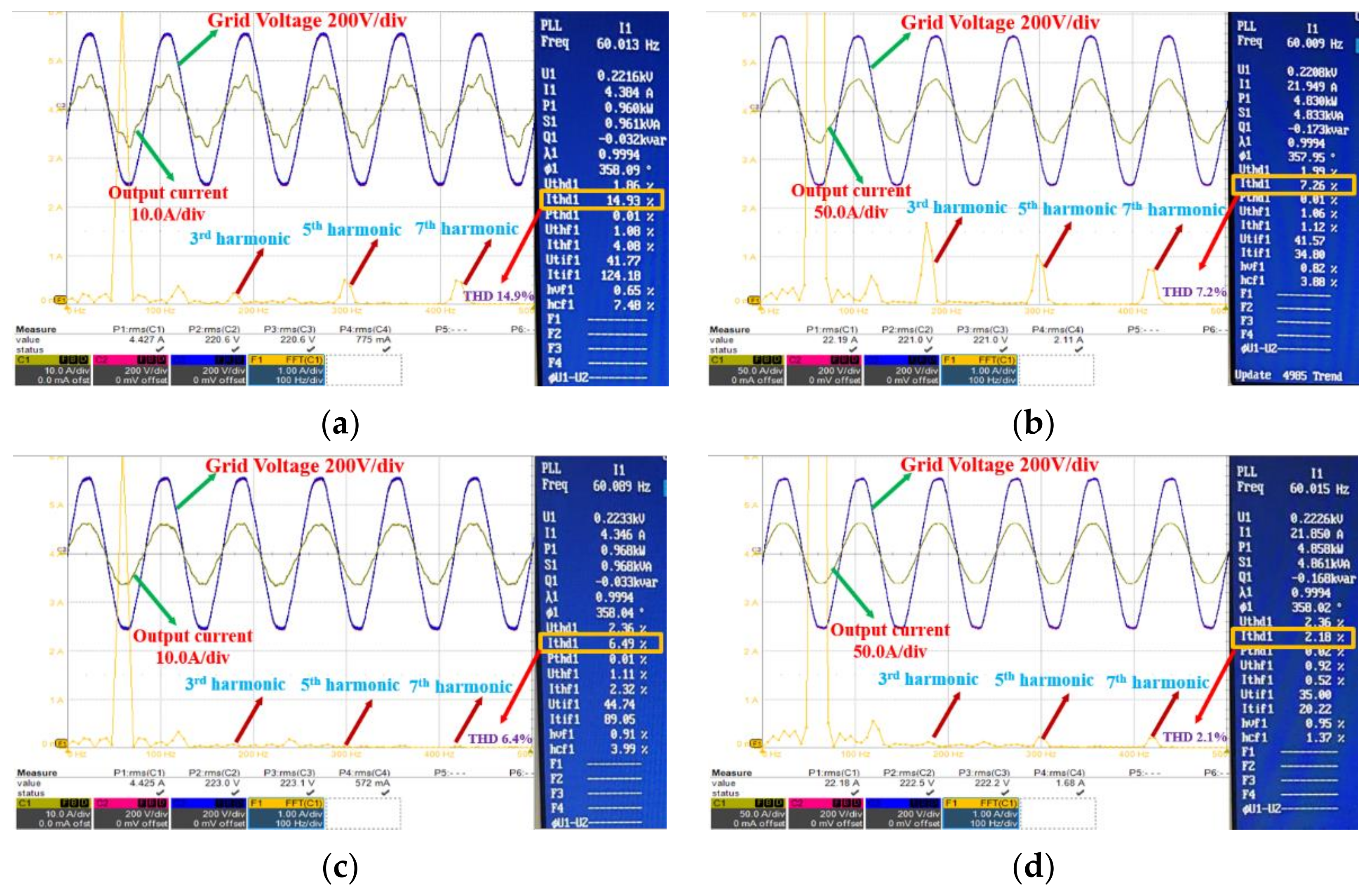
| 1 kW | 14.9% | 6.4% | 57% |
| 2 kW | 8.6% | 4.0% | 54% |
| 3 kW | 8.0% | 2.8% | 65% |
| 4 kW | 7.84% | 2.3% | 70% |
| 5 kW | 7.26% | 2.1% | 71% |
Publisher’s Note: MDPI stays neutral with regard to jurisdictional claims in published maps and institutional affiliations. |
© 2021 by the authors. Licensee MDPI, Basel, Switzerland. This article is an open access article distributed under the terms and conditions of the Creative Commons Attribution (CC BY) license (http://creativecommons.org/licenses/by/4.0/).
Share and Cite
Khan, R.A.; Ashraf, M.N.; Choi, W. A Harmonic Compensation Method Using a Lock-In Amplifier under Non-Sinusoidal Grid Conditions for Single Phase Grid Connected Inverters. Energies 2021, 14, 597. https://doi.org/10.3390/en14030597
Khan RA, Ashraf MN, Choi W. A Harmonic Compensation Method Using a Lock-In Amplifier under Non-Sinusoidal Grid Conditions for Single Phase Grid Connected Inverters. Energies. 2021; 14(3):597. https://doi.org/10.3390/en14030597
Chicago/Turabian StyleKhan, Reyyan Ahmad, Muhammad Noman Ashraf, and Woojin Choi. 2021. "A Harmonic Compensation Method Using a Lock-In Amplifier under Non-Sinusoidal Grid Conditions for Single Phase Grid Connected Inverters" Energies 14, no. 3: 597. https://doi.org/10.3390/en14030597
APA StyleKhan, R. A., Ashraf, M. N., & Choi, W. (2021). A Harmonic Compensation Method Using a Lock-In Amplifier under Non-Sinusoidal Grid Conditions for Single Phase Grid Connected Inverters. Energies, 14(3), 597. https://doi.org/10.3390/en14030597