Abstract
An interior permanent magnet synchronous motor (IPMSM) drive system with machine learning-based maximum torque per ampere (MTPA) as well as flux-weakening (FW) control was developed and is presented in this study. Since the control performance of IPMSM varies significantly due to the temperature variation and magnetic saturation, a machine learning-based MTPA control using a Petri probabilistic fuzzy neural network with an asymmetric membership function (PPFNN-AMF) was developed. First, the d-axis current command, which can achieve the MTPA control of the IPMSM, is derived. Then, the difference value of the dq-axis inductance of the IPMSM is obtained by the PPFNN-AMF and substituted into the d-axis current command of the MTPA to alleviate the saturation effect in the constant torque region. Moreover, a voltage control loop, which can limit the inverter output voltage to the maximum output voltage of the inverter at high-speed, is designed for the FW control in the constant power region. In addition, an adaptive complementary sliding mode (ACSM) speed controller is developed to improve the transient response of the speed control. Finally, some experimental results are given to demonstrate the validity of the proposed high-performance control strategies.
1. Introduction
IPMSMs have many attractive characteristics, including wide speed operating range, high-power density, and high torque-to-inertia ratio. Thus, IPMSMs has been utilized in many industrial applications [1,2,3,4]. However, the control characteristic of IPMSMs tends to time-varying behavior due to the machine parameters variation caused by the magnetic saturation.
For the IPMSM, the quadrature-axis inductance is increased by the rotor magnetic circuit saliency, which leads to a reluctance torque term incorporating into the torque equation [5]. However, to utilize the advantage of the reluctance torque term in the constant torque and constant power region, appropriate control methods are required. Therefore, an MTPA control has been proposed to improve the torque output in the constant torque region [5,6,7,8,9,10]. In [8], the method of using the high-frequency variation of the output mechanical power combined with a fuzzy-logic controller to obtain the advance angle of the MTPA for an IPMSM was proposed.
Moreover, the method proposed in [9] injects a small virtual current angle signal to track the MTPA operating point and to generate the d-axis current command by utilizing the inherent characteristic of the MTPA operation. With model-based torque correction in [10], an accurate and efficient torque control, as well as robust torque response, can be achieved for the MTPA operation. However, there is no intelligent control method using a neural network to achieve MTPA control in the above literature.
FW control is mainly applied to the DC and AC motors operation above the rated speed in the constant power region. There are quite a few methods to achieve FW control, such as current control [11], voltage control [12,13] and flux control [14]. In [11], a robust nonlinear control technique to achieve a wide-speed-range operation of the IPMSM based on the MTPA and FW controls was presented. For the proposed nonlinear controller, the FW and MTPA schemes are used to control the d-axis stator current above and below the rated speed, respectively. Moreover, a model-based design method of a voltage phase controller for the IPMSM was presented in [12]. The voltage phase controller controls the torque only in a high-speed region where the inverter output voltage amplitude is saturated. Furthermore, in [13], a voltage feedback FW control scheme for vector-controlled IPMSM drive systems was considered. A voltage control loop is also designed in this study to limit the inverter output voltage to the maximum output voltage of the inverter at high-speed for the FW control.
Since the PNN possesses the probability density function estimator and Bayes classification rule, it has superior modeling performance and adaptability [15,16,17]. Moreover, the PFNN comprises both the merits of PNN and fuzzy logic [18]. Therefore, many researchers have used PFNN to design advanced controllers and model represent complex plants [16,19]. Furthermore, PN is capable of analytical, graphical and mathematical modeling and is widely utilized to analyze the behavior of discrete event systems [20,21,22]. In addition, the learning capability of the neural networks can be upgraded, and the number of fuzzy rules can be further reduced by extending the dimension of the membership functions to AMFs [23]. A PPFNN-AMF, which possesses the merits of the PFNN, PN and the AMFs, was proposed in [23] and is adopted in this study to estimate the difference value of the dq-axis inductance of the IPMSM.
In recent years, SMC has attracted much attention because of its strong robustness and rapid control response to time-varying uncertainties, including internal parameter variations and external disturbances [24,25,26,27,28,29]. However, the disadvantage of SMC is the chattering phenomenon owing to the switching function [24,25]. In order to decrease the chattering phenomenon, many methods such as CSMC have been used. The CSMC can not only reduce the chattering phenomenon but also has good control accuracy [26,27]. On the other hand, it is necessary to have the boundary of the uncertainty for the design of CSMC, but it is difficult to obtain in advance in practical applications. Therefore, many nonlinear controllers combining with intelligent control or adaptive control to estimate the uncertainty of IPMSM have been proposed [27,28,29,30]. However, there is seldom research of the SMC methodologies considering the effect of reluctance torque of the IPMSM. To improve the robust control performance of the IPMSM drive system under parameter variations and external disturbances, an ACSM speed controller considering nonzero d-axis current is proposed in this study to improve the control performance.
A high-performance IPMSM drive system with intelligent MTPA based on PPFNN-AMF and FW control is proposed in this study. The PPFNN-AMF is utilized in this study to learn the difference value of the dq-axis inductance of the IPMSM. It can ensure that the correct difference value of the inductance is obtained under different operating conditions for the MTPA control. Furthermore, a voltage control loop is designed for the FW control. In addition, an ACSM speed controller considering nonzero d-axis current is proposed to improve the robustness of the speed control. Lyapunov stability theorem is used to derive the adaptive law, which is used for online estimation of the lumped uncertainty to ensure that the ACSM speed controller is asymptotically stable. The rest of this study is organized as follows: The theories and modeling of the MTPA and FW controls of the IPMSM drive are presented in Section 2, and the ACSM speed controller is developed in Section 3. The network structure and learning algorithms of the PPFNN-AMF are presented in Section 4. Some test cases with different speed commands and various load torques are investigated to verify the accuracy and robustness of the proposed high-performance control methods in Section 5. Finally, some conclusions are presented in Section 6.
2. MTPA and FW Control of IPMSM Drive
Figure 1 is the block diagram of the intelligent MTPA and FW-controlled IPMSM drive system with ACSM speed controller. First, the actual rotor position of the motor is determined by the encoder, and the mechanical speed is obtained by differentiating . Next, the mechanical speed is subtracted from the mechanical speed command to derive the mechanical speed error . Then, is inputted into the ACSM speed controller to get the q-axis current command . Moreover, the two inputs and one output PPFNN-AMF is adopted to learn the difference value of the dq-axis inductance and . The inputs of the PPFNN-AMF are and , and the output is the learning result of the dq-axis inductance differences , which is substituted into the MTPA formula to derive the d-axis current command for the MTPA control. While the FW control proceeds, the motor speed will be increased above the rated speed. The input of the MTPA block shown in Figure 1 will be switched to FW, and the will be kept constant during the FW control. Furthermore, to make sure that the stator voltage command will not exceed the voltage limit of the inverter is inputted into a PI controller to generate the variation of the d-axis current command , which is a negative value. Only when the inverter output voltage exceeds the maximum output voltage of the inverter, the input of the PI controller will be nonzero. That is to say, the output of the limiter shown in Figure 1 is zero when the input to the limiter is positive.
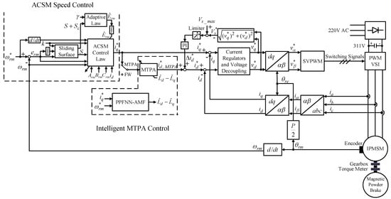
Figure 1.
Block diagram of intelligent maximum torque per ampere (MTPA) and flux-weakening (FW)-controlled interior permanent magnet synchronous motor (IPMSM) drive system with adaptive complementary sliding mode (ACSM) speed controller.
As shown in Figure 1, the three-phase currents and of the VSI are transformed to the corresponding q-axis current and d-axis current by using the coordinate transformation. In addition, and are subtracted, respectively from and , and then the dq axis voltage commands and are obtained through the PI controllers of the current loop. After and are obtained, and are derived by using the coordinate transformation. Moreover, the switching signals for the IGBTs of the VSI are generated through the SVPWM, and the switching frequency is 10 kHz. Finally, the switching signals are sent to the IGBTs to achieve intelligent MTPA and FW control.
2.1. MTPA Control
The electromagnetic torque of an IPMSM in the dq synchronous frame can be expressed as follows [5]:
where is the PM flux linkage; denotes the number of poles. First, define the relationship of the stator current between the dq-axis currents and
Substituting (2) into (1) gives the following relationship:
The d-axis current command of MTPA can be obtained by differentiating the electromagnetic torque equation with respect to the q-axis current and setting the derivative to zero to obtain the extreme value. The resultant equation is as follows:
Since the parameters of the IPMSM are not constant resulting from the effects of magnetic saturation, the measuring method of the dq-axis inductance differences will be developed, and the PPFNN-AMF will be adopted to learn the inductance differences in the constant torque region.
2.2. Estimation of Permanent-Magnet Flux Linkage
Owing to the magnetic saturation of the rotor core, the value of the q-axis inductance is mainly affected by the changing of the air gap flux. Therefore, the value of should be estimated online in order to accomplish the desired MTPA control performance. In this study, the inductance difference is estimated online instead of the and the PPFNN-AMF will be adopted to learn the inductance differences. Before measuring , it is necessary to estimate the value of the permanent-magnet flux linkage first. Since the measuring methods of , and are usually very complex [31,32], a heuristic method is developed in this section to generate the training data for the offline training of the PPFNN-AMF.
Let be zero first, then (1) can be simplified as:
Add two different load torques and to IPMSM, respectively, then (5) can be expressed as:
where is the friction torque; is the q-axis current when is added; is the q-axis current when is added; is the estimated permanent-magnet flux linkage. Then, subtract (6) from (7), and one can get
According to (8), the can be obtained as follows under any load torque conditions:
After is obtained, the measuring method of the will be illustrated in detail in the next section.
2.3. Measuring Method of dq-Axis Inductance Differences
Let be zero again, and define a new operating condition as follows:
where and are the electromagnetic torque and q-axis current of the new operating condition when . Then, without changing the load torque and the motor speed, define to generate reluctance torque of IPMSM and (1) can be rewritten as:
where is the q-axis current when . Since the operating conditions are the same, (10) and (11) are equal and can be expressed as:
According to (12), the dq-axis inductance differences can be obtained as follows using the estimated permanent-magnet flux linkage under any operating condition:
The PPFNN-AMF is utilized in this study to learn the difference value of the dq-axis inductance of the IPMSM. Therefore, to ensure effective offline training under different operating conditions, the q-axis current command and mechanical speed command are the input data, and the corresponding is the desired output for the offline training of the PPFNN-AMF. Then, under the real-time motor operation, the output of the trained PPFNN-AMF, which is the estimated dq-axis inductance difference , is substituted into (4) to derive the d-axis current command for the MTPA control in the constant torque region.
2.4. FW Control
The voltage model of an IPMSM in the dq synchronous frame can be written as [5]:
When the IPMSM is operated in the FW region at the steady-state condition, the voltage drop caused by the stator resistance in (14) can be neglected. Then, the dq voltage model of an IPMSM can be rewritten as follows:
Moreover, the flux model of an IPMSM in the dq synchronous frame can be described by [5]:
It is known from (18) that the principle of FW control is to let negative to generate the flux in the opposite direction of the PM to reduce and decrease the back EMF of an IPMSM in the constant power region. This allows IPMSM to continue to increase the rotor speed above the rated speed until the stator voltage command reaches the voltage limit of the inverter. To make sure that the inverter output voltage will not exceed the maximum output voltage of the inverter is inputted into a PI controller to generate the variation of d-axis current command , which is a negative value. On the other hand, the output of the limiter is zero when the input of the limiter is positive. After this, is added to to make the more negative to ensure that is less than as shown in Figure 1.
3. ACSM Speed Controller
The block diagram of the proposed ACSM speed controller, where the d-axis current is nonzero, is also shown in Figure 1. The mechanical dynamic equation of an IPMSM can be expressed as follows:
where J is the moment of inertia of the IPMSM; B is the damping coefficient; is the load torque. By neglecting the load torque, (20) can be modified as:
The dynamic of an IPMSM drive system can be formulated by using (1) and (21) as follows:
where ; ; ; , , , and are the nominal values of damping coefficient, moment of inertia, PM flux linkage, d-axis inductance and q-axis inductance, respectively. By considering the uncertainty, including the existence of parameter variations and external disturbances of the IPMSM drive system, (22) can be rewritten as:
where ; , , and are the time-varying parameter variations; is the lumped uncertainty and defined as:
is assumed to be bounded
where ρ is a given positive constant. Define the speed tracking error as follows:
Then, one can define the generalized sliding surface as follows:
where k is a positive constant. From (27) and (23), the following equation can be obtained:
Next, a second sliding surface, known as complementary sliding surface, is designed as follows [27]:
With the same positive constant k, an important result concerning the relationship between S and can be obtained in the following [27]:
Theorem 1.
For the system dynamic equation represented by (24), the stability of the proposed ACSM control system can be guaranteed, and the tracking error will reach and converge to a neighborhood of zero in finite time by using the proposed ACSM control law designed as (31). Moreover, the control law shown in (31) is a combination of an equivalent control law designed as (32) and a hitting control law designed as (33),
where sat is the saturation function with the boundary layer thickness[33] and is designed to reduce the chattering phenomena. The saturation function is defined as follows:
A Lyapunov function is chosen as
where V is a positive definite function;;is the estimated value of the; γ is a positive constant. Taking the time derivative of the Lyapunov function and using (29) and (30), one can obtain
Therefore, according to (36), the ACSM control lawand adaptive laware designed as follows:
The time derivative of the Lyapunov function can be formulated by (36) and (38) as follows:
Using (31)–(33) and (39), one can obtain
Since;is negative semidefinite, i.e.,, which means thatandare bounded. Now, one can define the following term:
then
Furthermore, becauseis bounded andis nonincreasing and bounded, the following result can be obtained:
In addition,is also bounded. Then,is uniformly continuous. Using Barbalat’s lemma [33], the following result can be derived:
Thus, (44) means thatandwill converge to zero as. Moreover,and. Therefore, the ACSM system guarantees the asymptotic stability of the speed tracking error, even if the parameter variations, external disturbances, and friction force exist.
4. PPFNN-AMF
The PPFNN-AMF proposed in [23] was utilized in this study to estimate the difference value of the dq-axis inductance of the IPMSM. The network structure and learning algorithms are presented in the following paragraphs.
4.1. Network Structure
There are six layers, which consist of the input, membership, Petri, probabilistic, rule and output layers with two inputs and one output in the network structure of the PPFNN-AMF shown in Figure 2a. The signal propagation of each layer is described in detail in the following:
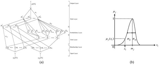
Figure 2.
Petri probabilistic fuzzy neural network with an asymmetric membership function (PPFNN-AMF): (a) Network structure; (b) asymmetric Gaussian function in the membership layer.
Input layer:
The input and the output of the node of the input layer are represented as follows:
where denotes the ith input to the input layer; N denotes the Nth iteration. The inputs of the PPFNN-AMF are and , which are the mechanical speed and the q-axis current command, respectively.
4.1.1. Membership Layer
The asymmetric Gaussian functions were adopted as the membership function in each node of this layer to implement the fuzzification operation shown in Figure 2b. In addition, the input and output of the node are expressed in the following:
In (46) and (47), and represent the input and the output of the membership layer. Moreover, denotes the mean of the asymmetric Gaussian function in the jth term associated with the ith input variable. Furthermore, and represent the left-hand-side and right-hand-side standard deviations of the asymmetric Gaussian function in the jth term associated with the ith input variable.
4.1.2. Petri Layer
In this layer, the transition is fired or unfired by the following equations:
where is the transition, is a threshold value, and is varied by the function ; and are positive constants. The relationship between the input and output of the Petri layer is presented as follows:
4.1.3. Probabilistic Layer
The receptive field function is a Gaussian function in the probabilistic layer and described as follows:
In (52) and (53), and denote the mean and standard deviation of the Gaussian function, and denotes its output.
4.1.4. Rule Layer
The node input and the node output of the rule layer are described as:
In (54)–(56), superscript I denotes the input, subscript l denotes the node number, and superscript o indicates the output. Moreover, and represent the inputs of rule layer; , which is set to 1, represents the connective weight between the membership layer and the rule layer; , which is also set to 1, represents the connective weight between the probabilistic layer and the rule layer; represents the output of the rule layer.
4.1.5. Output Layer
In the output layer, the node is denoted by performing the summation operation. Hence, the output of this layer, which is the estimated dq-axis inductance difference , is given as follows:
4.2. Learning Algorithms
In order to illustrate the learning algorithms of the PPFNN-AMF, first, the energy function is defined as:
where is the desired output.
Then, the learning algorithms are explained as follows:
4.2.1. Output Layer
The error term, which is propagated back from the output layer, is computed as:
According to the chain rule, the connective weight is updated by the amount:
where is the learning rate and the connective weight is updated as follows:
The error term to be propagated is calculated as follows:
4.2.2. Membership Layer
In this layer, the error term needs to be calculated and propagated as follows:
The mean of the asymmetric Gaussian function is defined and calculated as follows:
where denotes the learning rate of the mean of the asymmetric Gaussian function. Moreover, the left-hand-side and right-hand-side standard deviations of the asymmetric Gaussian function are calculated in the following:
where , represent the learning rates of the left-hand-side and right-hand-side standard deviations of the asymmetric Gaussian function, respectively. Therefore, the mean and the left-hand-side and right-hand-side standard deviations of the asymmetric Gaussian function are updated according to the following equations:
The exact calculation of the Jacobian of the system, which is contained in , is very difficult in practical applications. Thus, a delta adaptation law is proposed in the following
The detailed convergence analysis of the PPFNN-AMF can be referred to [23].
5. Experimental Results
To facilitate the verification of the proposed control strategies, the IPMSM test platform and the experimental drive system are shown in Figure 3. The IPMSM test platform comprised the IPMSM, the gearbox (with gear ratio 4:1), the torque meter and the magnetic powder brake. The total moment of inertia of the motor test platform was Nm/(rad/s2). The detailed information of the magnetic powder brake and IPMSM is listed in Table 1 and Table 2. The DSP -based motor drive included the DSP control boards, and PWM VSI are also shown in Figure 3. A torque meter with 100 Nm/7000 rpm was utilized for the measurement of the load torque. The resolution of the adopted encoder is only 8000 pulsed/rotation. Moreover, the maximum speed of the IPMSM in the experimentation was 3750 rpm in the constant power region. By using the gearbox with a gear ratio of 4:1 to reduce the speed, the maximum speed of the magnetic powder brake 937.5 rpm was smaller than the rated speed of the magnetic powder brake 1800 rpm. Furthermore, the ratings of the VSI using IGBTs was 5 kW/220 V/14 A. The switching frequency of 10 kHz was controlled by using SVPWM technology. The DC link voltage provided by an adjustable DC power supply was set at 311 V. According to the SVPWM, the inverter maximum output voltage was set to . In addition, the experimental cutoff frequency of the IPMSM drive system, including the motor test platform with ACSM speed controller, was about 30 Hz, which could be obtained by using an Agilent 35670A dynamic signal analyzer. The low bandwidth was due to the large inertial of the motor test platform, which includes IPMSM, gear, torque meter and magnetic powder brake, and the low-resolution of the adopted encoder. Since the moment of inertia of the IPMSM was Nm/(rad/s2), the resultant load moment of inertia ratio was 2.44:1.
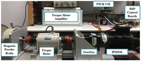
Figure 3.
Photo of the experimental setup.

Table 1.
Parameters of magnetic powder brake.
Table 2.
Parameters of IPMSM.
The controllers were implemented with a 120 MHz TMS320F28075 32-bit floating-point DSP to enhance computation performance of the proposed intelligent MTPA and FW control with ACSM speed control system. The flowcharts of the proposed ACSM controller and PPFNN-AMF are provided in Figure 4. Since the PPFNN-AMF was trained offline, the complexity was much reduced for the real-time implementation in the DSP. By using the clock tool of the Texas Instruments Code Composer Studio v6.2 program editing interface, the execution time of the “C” program could be obtained. The operation cycles and execution time for the proposed ACSM controller and PPFNN-AMF were 40 cycles (0.00033 ms) and 5252 cycles (0.0437 ms), respectively. Although the implemented complexity of the proposed ACSM controller and PPFNN-AMF were higher than that of the traditional PI controller and MTPA control, the execution time of the proposed ACSM controller was much less than the outer speed control loop time 1 ms (speed sampling time). Moreover, the execution time of the PPFNN-AMF was still less than the inner current control loop time of 0.1 ms (current sampling time).
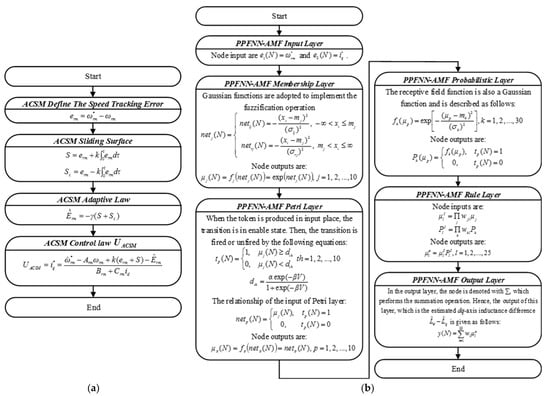
Figure 4.
Flowcharts of the proposed controllers in DSP: (a) ACSM speed controller; (b) PPFNN-AMF.
5.1. ACSM Speed Controller
Four cases of different parameters of the proposed ACSM speed controller shown in (31), (32) and (38) were tested from standstill to 500 rpm in order to verify the control performance. Case 1 was with k = 15, γ = 1; Case 2 was with k = 15, γ = 10; Case 3 was with k = 18, γ = 10; Case 4 was with k = 24, γ = 10.
The mechanical speed command , the mechanical speed , the mechanical speed error , and the q-axis current command in Cases 1 to 4 are shown in Figure 5, Figure 6, Figure 7 and Figure 8, respectively.
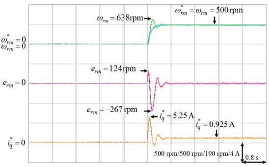
Figure 5.
Experimental results of ACSM speed controller from standstill to 500 rpm in Case 1.
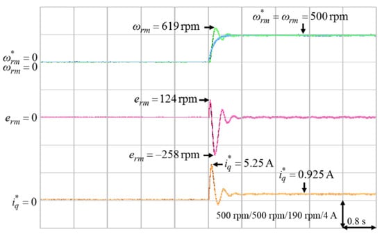
Figure 6.
Experimental results of ACSM speed controller from standstill to 500 rpm in Case 2.
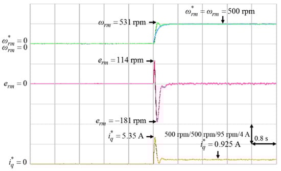
Figure 7.
Experimental results of ACSM speed controller from standstill to 500 rpm in Case 3.
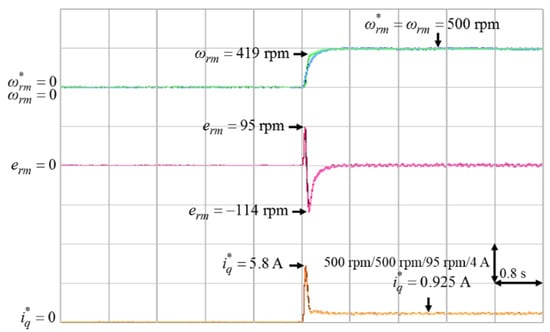
Figure 8.
Experimental results of ACSM speed controller from standstill to 500 rpm in Case 4.
According to Figure 5 and Figure 6, the parameter γ had little effect on the speed responses of the system. On the other hand, based on Figure 6, Figure 7 and Figure 8, the parameter k had a greater influence on the speed responses than the parameter γ. A larger k will make the mechanical speed error smaller, but it will cause larger q-axis current command. Therefore, the selection of the value of k was a tradeoff between speed response and starting current. In this study, in order to achieve the best control performance with the consideration of stability, the parameters of the ACSM speed controller were set to be k = 24, γ = 10 by trial and error.
5.2. PPFNN-AMF Estimator
As mentioned in Section 2.3, to ensure effective offline training under different operating conditions of load torque and speed, the q-axis current command and mechanical speed command were the input data, and the measured dq-axis inductance difference was the desired output for the offline training of the PPFNN-AMF. The training data, including 39 different , 13 different and 507 measured, are shown in Figure 9, and the training result after 10,000 epochs training of the PPFNN-AMF is shown in Figure 10. Since the measuring of all the training data was performed under nominal motor operating conditions, the temperature condition of all the obtained training data were the same as the experimentation shown in Figure 11, Figure 12, Figure 13, Figure 14 and Figure 15. In order to verify the training accuracy of PPFNN-AMF at different operating speed and load torque conditions, the training errors of five conditions are shown in Table 3. According to Table 3, the biggest training error was 1.689%. The rest training errors were all smaller than 1%, which could demonstrate that the PPFNN-AMF was well trained.
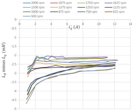
Figure 9.
Data of dq-axis inductance differences.
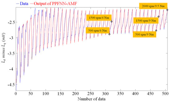
Figure 10.
Training result of PPFNN-AMF.
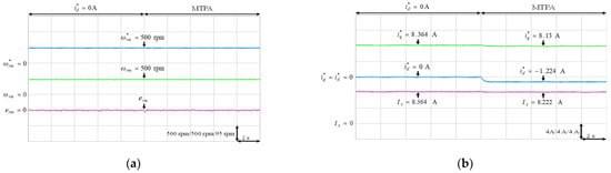
Figure 11.
Experimental results of MTPA control at 500 rpm with 6 Nm: (a) mechanical speed command, speed and speed error; (b) q-axis current command, d-axis current command and stator current.
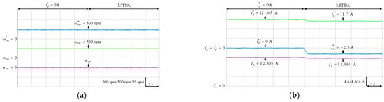
Figure 12.
Experimental results of MTPA control at 500 rpm with 9 Nm: (a) mechanical speed command, speed and speed error; (b) q-axis current command, d-axis current command and stator current.
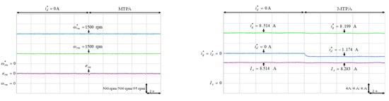
Figure 13.
Experimental results of MTPA control at 1500 rpm with 6 Nm: (a) mechanical speed command, speed and speed error; (b) q-axis current command, d-axis current command and stator current.
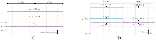
Figure 14.
Experimental results of MTPA control at 1500 rpm with 9 Nm: (a) mechanical speed command, speed and speed error; (b) q-axis current command, d-axis current command and stator current.
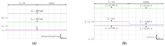
Figure 15.
Experimental results of MTPA control at 2000 rpm with 9.5 Nm: (a) mechanical speed command, speed and speed error; (b) q-axis current command, d-axis current command and stator current.
Table 3.
Training errors of PPFNN-AMF.
5.3. MTPA Control
After the PPFNN-AMF having been well trained offline, the output of the PPFNN-AMF could be substituted into the MTPA formula to get the d-axis current command of the MTPA under different operating conditions. Five test cases with different operating speed and load torque shown in Table 3 were selected to test the validity of the proposed intelligent MTPA control. The IPMSM was first operated with , and then the proposed MTPA control was performed at time s.
The experimental results of the MTPA control at (1) 500 rpm operating speed with 6 Nm and 9 Nm load torque; (2) 1500 rpm operating speed with 6 Nm and 9 Nm load torque; (3) rated speed 2000 rpm with rated torque 9.5 Nm, which was the rated output power 2 kW condition, were illustrated in Figure 11, Figure 12, Figure 13, Figure 14 and Figure 15, respectively. Figure 11a, Figure 12a, Figure 13a, Figure 14a and Figure 15a present the mechanical speed command , the mechanical speed and the mechanical speed error . The q-axis current command , the d-axis current command and the amplitude of stator current are shown in Figure 11b, Figure 12b, Figure 13b, Figure 14b and Figure 15b. In all test cased observed from Figure 11, Figure 12, Figure 13, Figure 14 and Figure 15, the intelligent MTPA control could effectively reduce the stator current with negative d-axis current command according to (4).
It was very difficult to verify the accuracy of the training data with the real data . Nevertheless, to verify the effectiveness of the proposed intelligent MTPA control at different operating conditions in Table 3, the d-axis current command was gradually changed from 0 A to −8 A to find out the lowest value of the stator current via experimentation [34]. The lowest value of the stator current, which could satisfy the specific operating condition in terms of speed and load torque, i.e., the MTPA operating point at that specific operating condition, could be obtained by varying the d-axis current command gradually as shown in Figure 16, Figure 17, Figure 18, Figure 19 and Figure 20. The experimental results of finding the lowest stator current at (1) 500 rpm operating speed with 6 Nm and 9 Nm load torque; (2) 1500 rpm operating speed with 6 Nm and 9 Nm load torque; (3). 2000 rpm with rated torque 9.5 Nm are illustrated in Figure 16, Figure 17, Figure 18, Figure 19 and Figure 20, respectively. The mechanical speed , the q-axis current command , the d-axis current command and the stator current are all presented in Figure 16, Figure 17, Figure 18, Figure 19 and Figure 20. Moreover, the experimental results of Figure 11, Figure 12, Figure 13, Figure 14, Figure 15, Figure 16, Figure 17, Figure 18, Figure 19 and Figure 20 are compared in Table 4. The stator currents of the proposed intelligent MTPA control shown in Figure 11, Figure 12, Figure 13, Figure 14, Figure 15 were quite close to the lowest values at all test cases shown in Figure 16, Figure 17, Figure 18, Figure 19, Figure 20, which could verify that the proposed IPMSM drive system could achieve effective MTPA control.
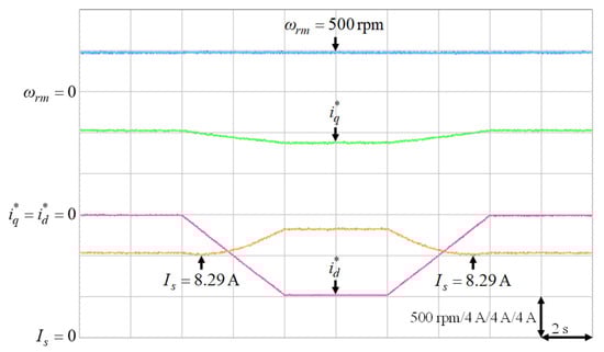
Figure 16.
Experimental results of finding the lowest stator current at 500 rpm with 6 Nm.
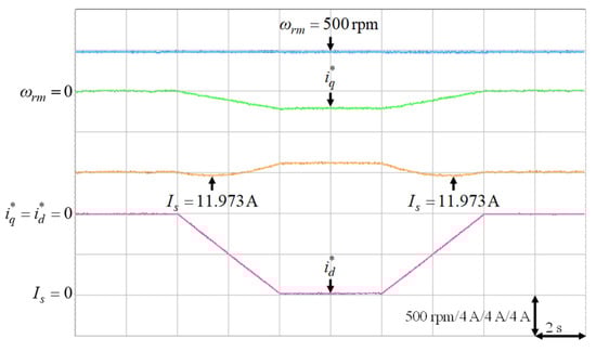
Figure 17.
Experimental results of finding the lowest stator current at 500 rpm with 9 Nm.
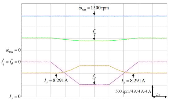
Figure 18.
Experimental results of finding the lowest stator current at 1500 rpm with 6 Nm.
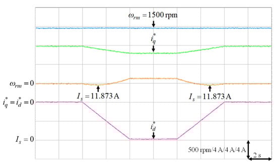
Figure 19.
Experimental results of finding the lowest stator current at 1500 rpm with 9 Nm.
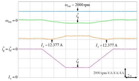
Figure 20.
Experimental results of finding the lowest stator current at 2000 rpm with 9.5 Nm.
Table 4.
Comparison of stator current amplitude.
5.4. FW Control
Some experimental results are provided to verify the effectiveness of the designed FW control for the operating speed above the rated speed. The parameters of the PI controller of the stator voltage controller are given as and where and represent the proportional and integral gains. These gains were tuned by trial and error to achieve the best transient response performance. Moreover, three FW operating conditions to achieve the constant power control, which were 3250 rpm under 5.85 Nm load torque, 3500 rpm under 5.43 Nm load torque and 3750 rpm under 5.07 Nm load torque, all at rated output power 2 kW, were tested. The IPMSM was first operated at 2000 rpm, and then the mechanical speed command was increased above the rated speed at time s. Figure 21, Figure 22 and Figure 23 depict the experimental resulted of the FW control for the mechanical speed command from 2000 rpm to 3250 rpm under 5.85 Nm load torque, 2000 rpm to 3500 rpm under 5.43 Nm load torque and 2000 rpm to 3750 rpm under 5.07 Nm load torque, respectively. Figure 21a, Figure 22a and Figure 23a present the mechanical speed command , the mechanical speed , the stator current and the stator voltage command . Furthermore, the q-axis current command , the d-axis current command of MTPA, the d-axis current command and the variation of d-axis current command are shown in Figure 21b, Figure 22b and Figure 23b. From the experimental resulted, once the inverter output voltage exceeds the maximum output voltage of the inverter, the output of the PI controller were negative. Then the output of the limiter, which was the variation of the d-axis current command , was added to to made the more negative to ensure that was less than . The resultant were −2.215 A, −5.313 A and −9.188 A for 3250 rpm, 3500 rpm and 3750 rpm, respectively. Therefore, the FW control with rated output power could be achieved at high-speed by increasing the negative d-axis current according to the designed voltage control loop for the FW control.
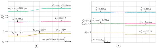
Figure 21.
Experimental results of FW control from 2000 rpm to 3250 rpm under 5.85 Nm load torque: (a) Mechanical speed command, mechanical speed, stator current and stator voltage command; (b) q-axis current command, d-axis current command of MTPA, d-axis current command and variation of d-axis current command.
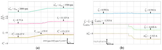
Figure 22.
Experimental results of FW control from 2000 rpm to 3500 rpm under 5.43 Nm load torque: (a) Mechanical speed command, mechanical speed, stator current and stator voltage command; (b) q-axis current command, d-axis current command of MTPA, d-axis current command and variation of d-axis current command.
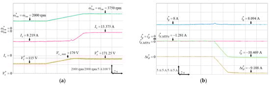
Figure 23.
Experimental results of FW control from 2000 rpm to 3750 rpm under 5.07 Nm load torque: (a) mechanical speed command, mechanical speed, stator current and stator voltage command; (b) q-axis current command, d-axis current command of MTPA, d-axis current command and variation of d-axis current command.
6. Conclusions
An IPMSM drive system with machine learning-based MTPA control in the constant torque region and an FW control in the constant power region was successfully developed in this study.
Moreover, an ACSM speed controller was developed to improve the transient response of the speed control. In the intelligent MTPA control, first, the d-axis current command which can achieve the MTPA control was derived. Then, the difference value of the dq-axis inductance of the IPMSM was obtained by a well-trained PPFNN-AMF and substituted into the formula of d-axis current command to achieve the MTPA control and to alleviate the effect of the magnetic saturation. In the FW control, a voltage control loop was designed to limit the inverter output voltage to the maximum output voltage of the inverter by increasing the negative d-axis current at high-speed. Finally, some experimental results were provided to demonstrate the validity of the proposed high-performance control strategies of the IPMSM drive system, including the ACSM speed control, the intelligent MTPA control and the FW control.
The main contributions of this study are listed as follows: (1) An ACSM speed controller considering nonzero d-axis current was proposed to improve the robustness of the speed control. Moreover, the Lyapunov stability theorem was used to derive the adaptive law, which was used for online estimation of the lumped uncertainty. (2) The PPFNN-AMF was adopted in this study to learn the difference value of the dq-axis inductance of the IPMSM offline. After the PPFNN-AMF was well-trained, the difference value of the dq-axis inductance of the IPMSM was obtained by the PPFNN-AMF and substituted into the d-axis current command of the MTPA to alleviate the saturation effect in the constant torque region. (3) The successful implementation of the intelligent MTPA and FW control with the proposed ACSM speed controller in a 32-bit floating-point DSP was built to achieve the MTPA and FW control at different speeds and load torque conditions for an IPMSM drive.
Author Contributions
F.-J.L. and Y.-H.L. designed and developed the main parts of research work including theory derivation and analyses of the obtained results. F.-J.L. and Y.-H.L. were also mainly responsible for preparing the paper. J.-R.L. and W.-T.L. contributed in DSP-based control platform and writing parts. All authors have read and agreed to the published version of the manuscript.
Funding
This research was funded by Ministry of Science and Technology of Taiwan, R.O.C., through its grant number MOST 107-2221-E-008-078-MY3.
Data Availability Statement
Data sharing not applicable. No new data were created or analyzed in this study. Data sharing is not applicable to this article.
Conflicts of Interest
The authors declare no conflict of interest.
Nomenclature
| IPMSMs | Interior permanent magnet synchronous motors |
| MTPA | Maximum torque per ampere |
| FW | Flux-weakening |
| PNN | Probabilistic neural network |
| PFNN | Probabilistic fuzzy neural network |
| PN | Petri net |
| AMFs | Asymmetric membership functions |
| PPFNN-AMF | Petri probabilistic fuzzy neural network with an asymmetric membership function |
| SMC | Sliding mode control |
| CSMC | Complementary sliding mode control |
| ACSM | Adaptive complementary sliding mode |
| VSI | Voltage source inverter |
| IGBTs | Insulated-gate bipolar transistors |
| SVPWM | Space vector pulse width modulation |
| PM | Permanent-magnet |
| PI | Proportional-integral |
References
- Mwasilu, F.; Kim, E.K.; Rafaq, M.S.; Jung, J.W. Finite-set model predictive control scheme with an optimal switching voltage vector technique for high-performance IPMSM drive applications. IEEE Trans. Ind. Inform. 2018, 14, 3840–3848. [Google Scholar] [CrossRef]
- Li, K.; Wang, Y. Maximum torque per ampere (MTPA) control for IPMSM drives using signal injection and an MTPA control law. IEEE Trans. Ind. Inform. 2019, 15, 5588–5598. [Google Scholar] [CrossRef]
- Kim, E.K.; Kim, J.; Choi, H.H.; Jung, J.W. Variable structure speed controller guaranteeing robust transient performance of an IPMSM Drive. IEEE Trans. Ind. Inform. 2019, 15, 3300–3310. [Google Scholar] [CrossRef]
- Yang, D.; Mok, H.; Lee, J.; Han, S. Adaptive torque estimation for an IPMSM with cross-coupling and parameter variations. Energies 2017, 10, 167. [Google Scholar] [CrossRef]
- Lin, F.J.; Hung, Y.C.; Chen, J.M.; Yeh, C.M. Sensorless IPMSM drive system using saliency back-EMF-based intelligent torque observer with MTPA control. IEEE Trans. Ind. Inform. 2014, 10, 1226–1241. [Google Scholar]
- Pairo, H.; Shoulaie, A. Operating region and maximum attainable speed of energy-efficient control methods of interior permanent-magnet synchronous motors. IET Power Electron. 2017, 10, 555–567. [Google Scholar] [CrossRef]
- Jung, S.; Hong, J.; Nam, K. Current minimizing torque control of the IPMSM using Ferrari’s method. IEEE Trans. Power Electron. 2013, 28, 5603–5617. [Google Scholar] [CrossRef]
- Liu, T.H.; Chen, Y.; Wu, M.J.; Dai, B.C. Adaptive controller for an MTPA IPMSM drive system without using a high-frequency sinusoidal generator. IET J. Eng. 2017, 2017, 13–25. [Google Scholar] [CrossRef]
- Sun, T.; Wang, J.; Chen, X. Maximum torque per ampere (MTPA) control for interior permanent magnet synchronous machine drives based on virtual signal injection. IEEE Trans. Power Electron. 2015, 30, 5036–5045. [Google Scholar] [CrossRef]
- Liu, Q.; Hameyer, K. High-performance adaptive torque control for an IPMSM with real-time MTPA operation. IEEE Trans. Energy Convers. 2017, 32, 571–581. [Google Scholar] [CrossRef]
- Schoonhoven, G.; Nasir Uddin, M. MTPA- and FW-based robust nonlinear speed control of IPMSM drive using Lyapunov stability criterion. IEEE Trans. Ind. Appl. 2016, 52, 4365–4374. [Google Scholar] [CrossRef]
- Miyajima, T.; Fujimoto, H.; Fujitsuna, M. A precise model-based design of voltage phase controller for IPMSM. IEEE Trans. Power Electron. 2013, 28, 5655–5664. [Google Scholar] [CrossRef]
- Bolognani, S.; Calligaro, S.; Petrella, R. Adaptive flux-weakening controller for interior permanent magnet synchronous motor drives. IEEE J. Emerg. Sel. Top. Power Electron. 2014, 2, 236–248. [Google Scholar] [CrossRef]
- Chen, Y.; Huang, X.; Wang, J.; Niu, F.; Zhung, J.; Fang, Y.; Wu, L. Improved flux-weakening control of IPMSMs based on torque feedforward technique. IEEE Trans. Power Electron. 2018, 33, 10970–10978. [Google Scholar] [CrossRef]
- Hart, S.J.; Shaffer, R.E.; Rose-Pehrsson, S.L.; McDonald, J.R. Using physics-based modeler outputs to train probabilistic neural networks for unexploded ordnance (UXO) classification in magnetometry surveys. IEEE Trans. Geosci. Remote Sens. 2001, 39, 797–804. [Google Scholar] [CrossRef]
- Jin, X.; Srinivasan, D.; Cheu, R.L. Classification of freeway traffic patterns for incident detection using constructive probabilistic neural networks. IEEE Trans. Neural Netw. 2001, 12, 1173–1187. [Google Scholar] [CrossRef]
- Lin, F.J.; Lu, K.C.; Ke, T.H.; Li, H.Y. Reactive power control of three-phase PV system during grids faults using Takagi-Sugeno-Kang probabilistic fuzzy neural network control. IEEE Trans. Ind. Electron. 2015, 62, 5516–5528. [Google Scholar] [CrossRef]
- Wai, R.J.; Muthusamy, R. Design of fuzzy-neural-network inherited backstepping control for robot manipulator including actuator dynamics. IEEE Trans. Fuzzy Syst. 2014, 22, 709–722. [Google Scholar] [CrossRef]
- Lin, F.J.; Huang, M.S.; Yeh, P.Y.; Tsai, H.C.; Kuan, C.H. DSP-based probabilistic fuzzy neural network control for li-ion battery charger. IEEE Trans. Power Electron. 2012, 27, 3782–3794. [Google Scholar] [CrossRef]
- Murata, T. Petrinets: Properties, analysis and applications. Proc. IEEE 1989, 77, 541–580. [Google Scholar] [CrossRef]
- Kaur, K.; Rana, R.; Kumar, N.; Singh, M.; Mishra, S. A colored petri net based frequency support scheme using fleet of electric vehicles in smart grid environment. IEEE Trans. Power Syst. 2016, 31, 4638–4649. [Google Scholar] [CrossRef]
- Wang, P.; Ma, L.; Goverde, R.M.P.; Wang, Q. Rescheduling trains using Petri nets and heuristic search. IEEE Trans. Intell. Transp. Syst. 2016, 17, 726–735. [Google Scholar] [CrossRef]
- Lin, F.J.; Chen, S.G.; Li, S.; Chou, H.T.; Lin, J.R. Online auto-tuning technique for IPMSM servo drive by intelligent identification of moment of inertia. IEEE Trans. Ind. Inform. 2020, 16, 7579–7590. [Google Scholar] [CrossRef]
- Wang, Y.; Feng, Y.; Zhang, X.; Liang, J. A new reaching law for antidisturbance sliding-mode control of PMSM speed regulation system. IEEE Trans. Power Electron. 2020, 35, 4117–4126. [Google Scholar] [CrossRef]
- Wang, A.; Wei, S. Sliding mode control for permanent magnet synchronous motor drive based on an improved exponential reaching law. IEEE Access 2019, 7, 146866–146875. [Google Scholar] [CrossRef]
- Jin, H.; Zhao, X. Approach angle-based saturation function of modified complementary sliding mode control for PMLSM. IEEE Access 2019, 7, 126014–126024. [Google Scholar] [CrossRef]
- Lin, F.J.; Hung, Y.C.; Tsai, M.T. Fault-tolerant control for six-phase PMSM drive system via intelligent complementary sliding-Mode control using TSKFNN-AMF. IEEE Trans. Ind. Electron. 2013, 60, 5747–5762. [Google Scholar] [CrossRef]
- Liang, C.Y.; Su, J.P. A new approach to the design of a fuzzy sliding mode controller. Fuzzy Sets Syst. 2003, 139, 111–124. [Google Scholar] [CrossRef]
- Kim, E.; Kim, J.; Nguyen, H.T.; Choi, H.H.; Jung, J. Compensation of parameter uncertainty using an adaptive sliding mode control strategy for an interior permanent magnet synchronous motor drive. IEEE Access 2019, 7, 11913–11923. [Google Scholar] [CrossRef]
- Choi, H.H.; Vu, N.T.T.; Jung, J.W. Digital implementation of an adaptive speed regulator for a PMSM. IEEE Trans. Power Electron. 2011, 26, 3–8. [Google Scholar] [CrossRef]
- Rahman, M.M.; Uddin, M.N. Third harmonic injection based nonlinear control of IPMSM drive for wide speed range operation. IEEE Trans. Ind. Appl. 2019, 55, 3174–3184. [Google Scholar] [CrossRef]
- Xu, W.; Lorenz, R.D. High-frequency injection-based stator flux linkage and torque estimation for DB-DTFC implementation on IPMSMs considering cross-saturation effects. IEEE Trans. Ind. Appl. 2014, 50, 3805–3815. [Google Scholar] [CrossRef]
- Slotine, J.J.E.; Li, W. Applied Nonlinear Control; Prentice-Hall: Englewood Cliffs, NJ, USA, 1991. [Google Scholar]
- Kim, S.; Yoon, Y.; Sul, S.; Ide, K. Maximum torque per ampere (MTPA) control of an IPM machine based on signal injection considering inductance saturation. IEEE Trans. Power Electron. 2013, 28, 488–497. [Google Scholar] [CrossRef]
Publisher’s Note: MDPI stays neutral with regard to jurisdictional claims in published maps and institutional affiliations. |
© 2021 by the authors. Licensee MDPI, Basel, Switzerland. This article is an open access article distributed under the terms and conditions of the Creative Commons Attribution (CC BY) license (http://creativecommons.org/licenses/by/4.0/).