Article

Diagnostic Protocol for Thermal Performance of District Heating Pipes in Operation. Part 1: Estimation of Supply Pipe Temperature by Measuring Temperature at Valves after Shutdown

Department of Architecture and Civil Engineering, Chalmers University of Technology, SE-412 96 Gothenburg, Sweden
*
Author to whom correspondence should be addressed.
Energies 2021, 14(16), 5192; https://doi.org/10.3390/en14165192
Submission received: 18 July 2021 / Revised: 13 August 2021 / Accepted: 18 August 2021 / Published: 22 August 2021
(This article belongs to the Special Issue Recent Advances in District Heating)

Abstract

:
This study evaluates temperatures measured at district heating (DH) valves in manholes and their usability for non-destructively assessing the thermal performance of buried DH pipes. The study was conducted as a field test in which part of a DH network was shut down and the temperature decline in the valves was analysed in terms of absolute temperature and thermal response time from the DH pipe to the top of the valve. The calculated and measured supply pipe temperatures by the drainage valves were in good agreement, with 1% deviation. The valve measurement analysis from this study shows that the drainage valve has good potential to serve as a measurement point for assessing the thermal status of a DH network. However, the shutdown valve measurements were greatly affected by the manhole environment.

1. Introduction

District heating (DH) networks have been used for decades and their usage increased substantially in the 1960s in the USA and Europe. The pipe types used vary, but polyurethane (PUR)-insulated single pipes are very common [1]. The heat energy produced and delivered to customers is measured by the energy companies, so the heat losses throughout the whole network can be determined. In Sweden, around 10% of the energy supplied to DH networks is lost through heat losses from the distribution pipes [2], with aging and degradation of the PUR increasing the heat losses [3]. A common rigid DH pipe in a Swedish DH network consists of an inner service pipe of steel and an outer casing pipe of polyethylene (PE); between them is the PUR insulation, a gas-filled closed-cell structure.
As the pipes age, energy companies need to renew their DH networks. However, it is hard to assess the thermal status of an aged section, since the age by itself does not equal to poor insulation status. Thermography is a method used by energy companies to detect heat and especially water leakage, although it cannot assess the thermal status of pipe insulation with high resolution. The absence of a suitable non-destructive method for assessing the thermal performance of a network has previously been identified by the present authors [4]. To fill this research gap, a “cooling method” has been developed for use during network maintenance with an excavated pit [5,6,7]. This cooling method is based on the temporary shutdown of part of the pipe network, while the cooling process is registered by thermocouples to capture the temperature decline in the service pipe (i.e., supply pipe). Furthermore, the thermal status of the network can be calculated using the temperature decline of the supply pipe.
The purpose of this paper is to develop and evaluate a cooling method for assessing the thermal status of a DH network, focusing on an operating and unexcavated network. The method is based on measuring the temperatures of a shutdown valve and a drainage valve. The paper presents a thermal response time analysis of the valves during the cooling period. Furthermore, the supply pipe temperature before a shutdown is evaluated by estimating the time lag and temperature drop, using data collected from DH users on the network outside the evaluated part. The measurements evaluated in this study therefore create prerequisites for capturing the actual temperature in the supply pipe, which can be used for assessing the thermal status of a DH pipe section.

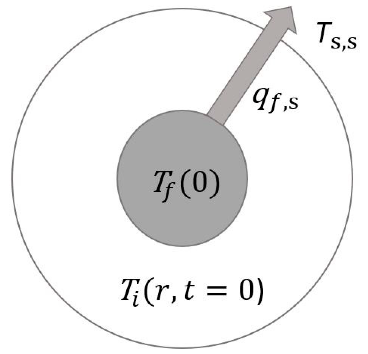
2. Concept for Developing the Cooling Method

For measurements of pipes excavated during maintenance, previously investigated by the authors [8], four possible measurement positions and the importance of accurate measurements were highlighted as the key to using the cooling method with high precision. For DH pipes in operation, the shutdown and drainage valves have been addressed as parts of the system where sensors could be placed. The measured value temperatures can be used for calculating the temperature decline of the DH pipe section. However, it is difficult to capture the actual absolute temperature in the supply pipe by means of valve measurements due to time lag of the valves and interactions with ambient air temperature in the manhole.
The initial temperature of a supply pipe, before a shutdown, is important for estimating the absolute temperature decline of the supply pipe during the cooling period. Energy companies measure the supply temperature at several points in a DH network, mainly at the customers’ DH centrals and at the heating plant in the outgoing supply water, i.e., the supply temperature is known before shutting down part of the network for thermal performance assessment. The distance from the supply temperature measurement points to assessed parts of the network will be case specific, and the accuracy of these temperature measurements is governed by the point-to-point heat losses.

2.1. Requirements

The cooling method concept involves shutting down a section of an operating DH network for a few hours, measuring temperatures at one or several points in a pipe section, and finally calculating the temperature decline along the section [8]. In this paper we are using two valves as measurement points, i.e., the drainage and shutdown valves, which are accessible via the manholes in a network.
The temperature decline along a supply pipe section during a shutdown, determined by measuring the temperature decline between the valves, is influenced by seasonal soil temperature variations, shutdown duration, the supply pipe temperature history, the supply pipe water volume, and the PUR insulation status anticipated by the method. We assume that the ambient temperature in the manhole will not influence the temperature of the observed supply pipe section during a shutdown period. However, the ambient air temperature in the manhole does influence the valve measurements and will therefore be considered in the valve temperature analysis.

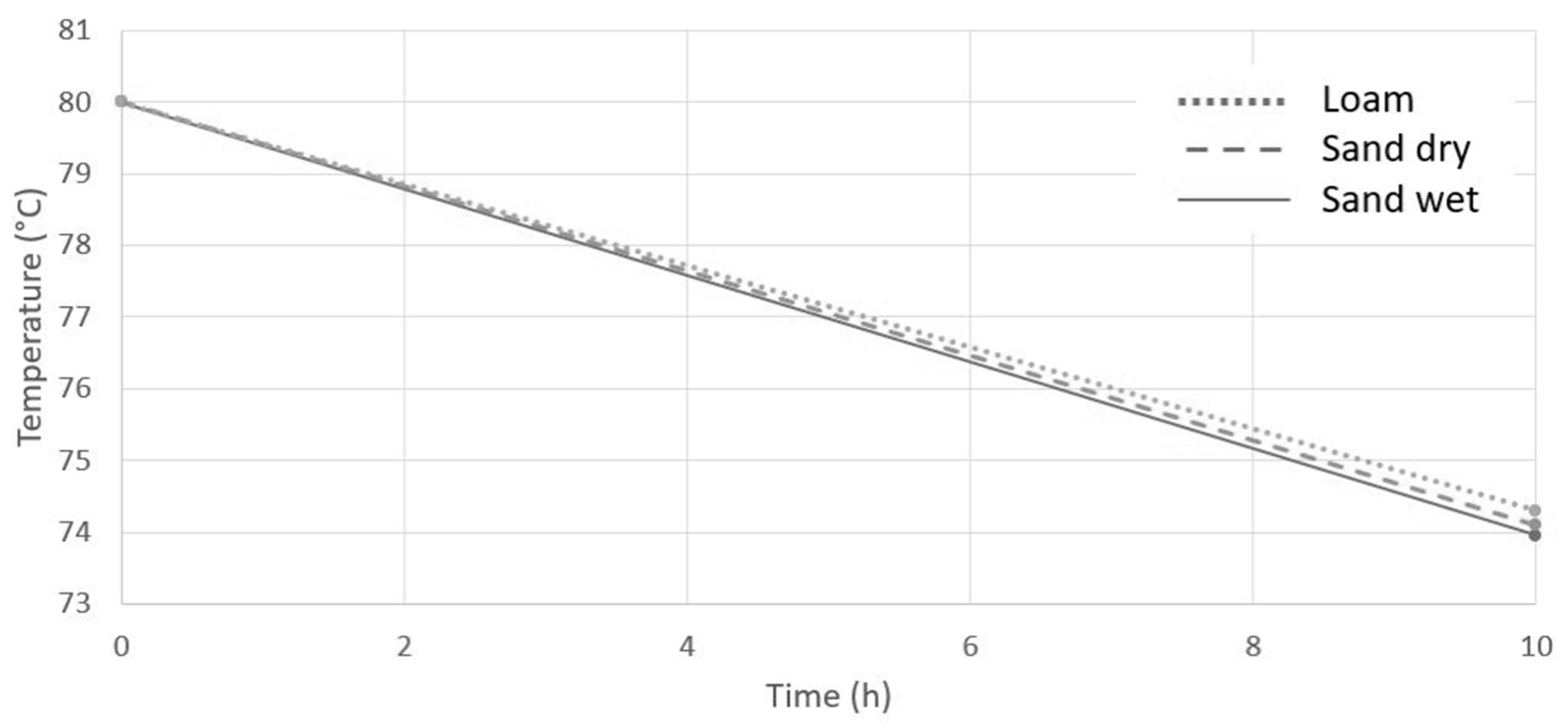
2.1.1. Influence of Seasonal Soil Temperature Variations on Estimating the Thermal Conductivity of the Pipe

The fluid temperature in the supply pipe is governed by the outgoing supply temperature from the DH plant and by the heat loss to the surroundings. The latter is determined by the fluid temperature itself and by the outdoor temperature. The annual average outdoor temperature and the seasonal variation amplitude constitute the main components of interest. The geometric dimensions of the pipe and the thermal properties of the insulation are of course also important for the heat loss magnitude. The annual average temperature in the supply pipe and the annual average outdoor temperature result in an average soil temperature around the pipe over the year. Superimposed on this is the seasonal variation in the soil temperature, the amplitude of which is much less than that of the outdoor temperature due to the dampening of the soil layer [9]. We can expect the temperature of the soil surrounding the pipe to be fairly stable over time, so the heat transfer from the DH pipe can be considered a quasi-steady-state condition.
Let us first assume that the supply pipe temperature and the soil temperature have been constant for a couple of days before the shutdown (see Figure 1). The impact of a non-stable temperature history and of short-term temperature variations on the time scale of hours and days will be investigated later in Section 2.1.3. The supply fluid temperature before time zero, i.e., the time of shutdown, is denoted T f ( 0 ) (K); the corresponding temperature in the surrounding insulation is denoted T i ( r , t = 0 ) (K), while the immediately surrounding soil temperature is T s , s . The quasi-steady-state heat flow through the pipe and into the soil is q f ,   s (W/m). The heat loss is balanced by the heat release due to the temperature drop along the length of the pipe, q f ( = q f , s ) .
Figure 2 shows how the heat transfer, after the shutdown, can be analysed by superposing two separate processes. The first panel on the left (a) depicts the total transient thermal problem to be solved. In the first process, shown in panel (b), the heat loss to the soil from the pipe at time zero, q f , s , continues to be balanced by the heat supply, q f . Additionally, as the initial temperature inside the pipe is the same as for the total process, the pipe temperatures will be the same as those before the shutdown. The second process in Figure 2, shown in panel (c), then needs to have a negative heat source, q f , to cancel out the heat supply, which must be zero after shutdown for the total process. The initial temperature inside the pipe is zero for the second process.
The heat transfer between the water and the insulation can be neglected over short periods, since these temperatures are both approximately zero. The temperature drop, i.e., the slope of the fluid temperature, d T f d t (K/m), over short periods, is therefore directly given by the following heat balance, Equation (1):
ρ c f A f d T f d t | t 0 = q f
Here, ρ c f (J/m3K) is the volumetric heat capacity of the water and A f (m2) is the cross-sectional area of the water pipe.
The estimated thermal conductivity, λ i (W/mK), of the pipe insulation, can then be calculated using Equation (2):
ρ c f A f d T f d t | t 0 = q s = 2 π λ i ln ( R o u t / R i n t ) T f , 0 T s
λ i ρ c f A f 2 π T f , 0 T s ln ( R o u t R i n t ) | d T f d t | t 0
Here, the outer casing pipe and inner supply pipe radii are R o u t (m) and R i n t (m), respectively.
Using superposition, the heat transfer process can be simulated numerically by coding a finite difference method (FDM) in MATLAB. The required shutdown time and influence of thermal history in the pipe can then be calculated if adequate assumptions are made as to the involved parameters, i.e., fluid temperatures, soil temperature, and thermal conductivity of PUR.

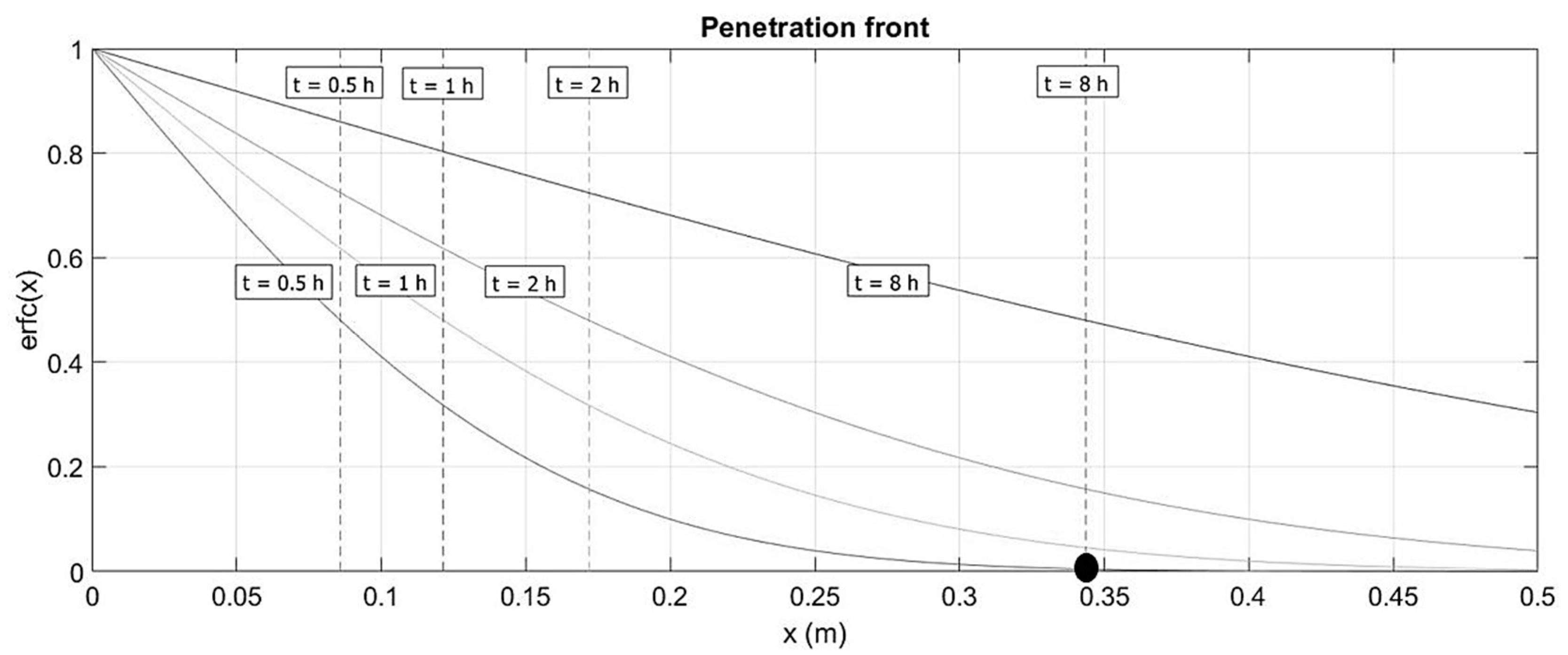
2.1.2. Shutdown Time

The required shutdown time depends on the dimensions of the pipes, due to the heat capacity of the water volume in the pipe and the insulation thicknesses and thermal properties. Previous work [6] indicates that a minimum of approximately 1–2 °C of temperature decline during the shutdown is required for a high-accuracy analysis, which partly depends on the use of high-precision measurement equipment. Figure 3 shows examples of the decline in the supply water temperature. The decline is approximately exponential, with a rapid temperature change at the beginning when the temperature difference between the water and the casing pipe/soil is large and slow when the temperature difference becomes smaller throughout the cooling phase. The supply temperature is assumed to be constant prior to shutdown. As seen in Figure 3, larger-dimension pipes such as DN500, in which the nominal diameter (i.e., the actual supply pipe diameter) is 508 mm, require approximately 8 h of shutdown time to reach a ΔT of 1 °C, whereas smaller-dimension pipes, such as DN100, require only 1 h to reach a ΔT of 1 °C (see Figure 3a,b).
To analyse the impact of the surrounding soil on the temperature decline after shutdown, the heat transfer process is simulated numerically using FDM in MATLAB as described above, now also accounting for the soil outside the DH pipe, extended to infinity. A starting soil temperature of 10 °C is assumed (annual mean temperature at the location) and the soil types are wet sand, dry sand, and loam, with a large range of thermal properties (see Table 1 and Figure 4).
Figure 4 depicts the shutdown of a DN200 pipe showing the only slightly varying impacts of the different soil types on the temperature decline, which was approximately 6 °C over 10 h for all soils. Hence, the impact of soil type on the shutdown time is small, with different pipe dimensions having more significant effects.

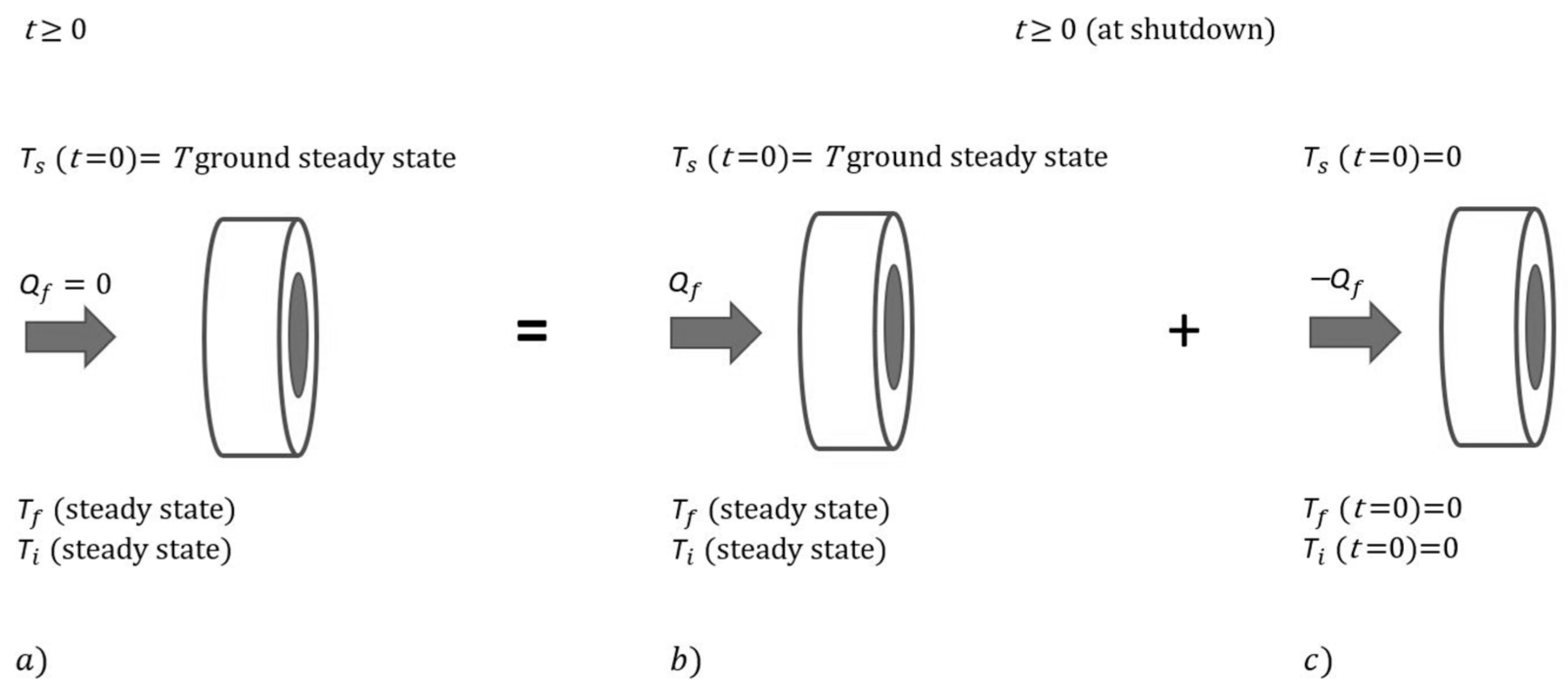
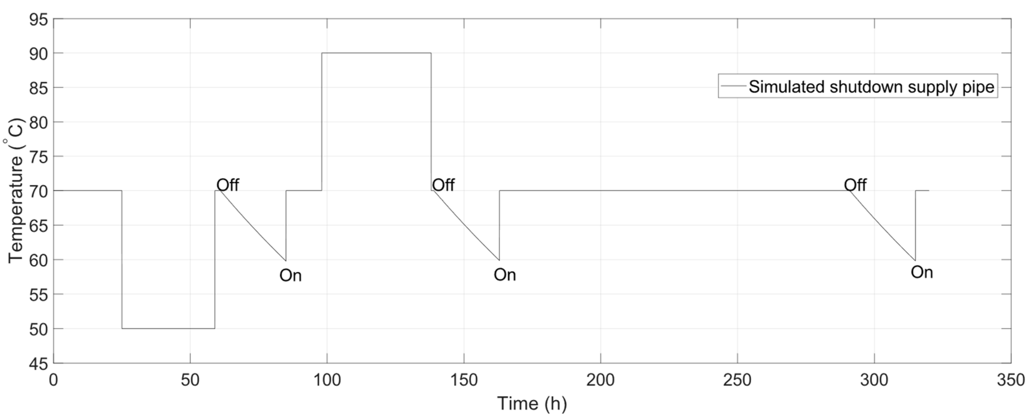
2.1.3. Influence of Thermal History of the Supply Pipe Temperature

The influence of the pre-shutdown thermal history of the supply water on the temperature decline in the pipe is investigated using numerical simulations. Temperatures and shutdown times are used for three simulated shutdowns using Equation (3), where u is dimensionless, T f ( t ) is the supply temperature during a shutdown, T f ( 0 ) is the supply temperature at the start of a shutdown, and T s is the temperature of the surrounding soil.
u = T f T s T f ( 0 ) T s
Three shutdowns of 24 h each are illustrated in Figure 5, showing various recent supply temperature histories: one with a recent increase of 10 °C after a low-temperature period prior to shutdown, one with a recent decrease of 10 °C after a high-temperature period, and one with a long period of stable temperatures. All histories start at 70 °C ( u = 1 ), decline with the same slope to 60 °C ( u = 0.83 ) , and after a longer period reach temperature balance with the surrounding soil ( u = 0 ).
Regardless of the thermal history, with increasing, decreasing, or constant temperatures in the supply pipe, the slopes of the temperature declines are approximately equal, thereby not affecting the shutdown time (see Figure 5).

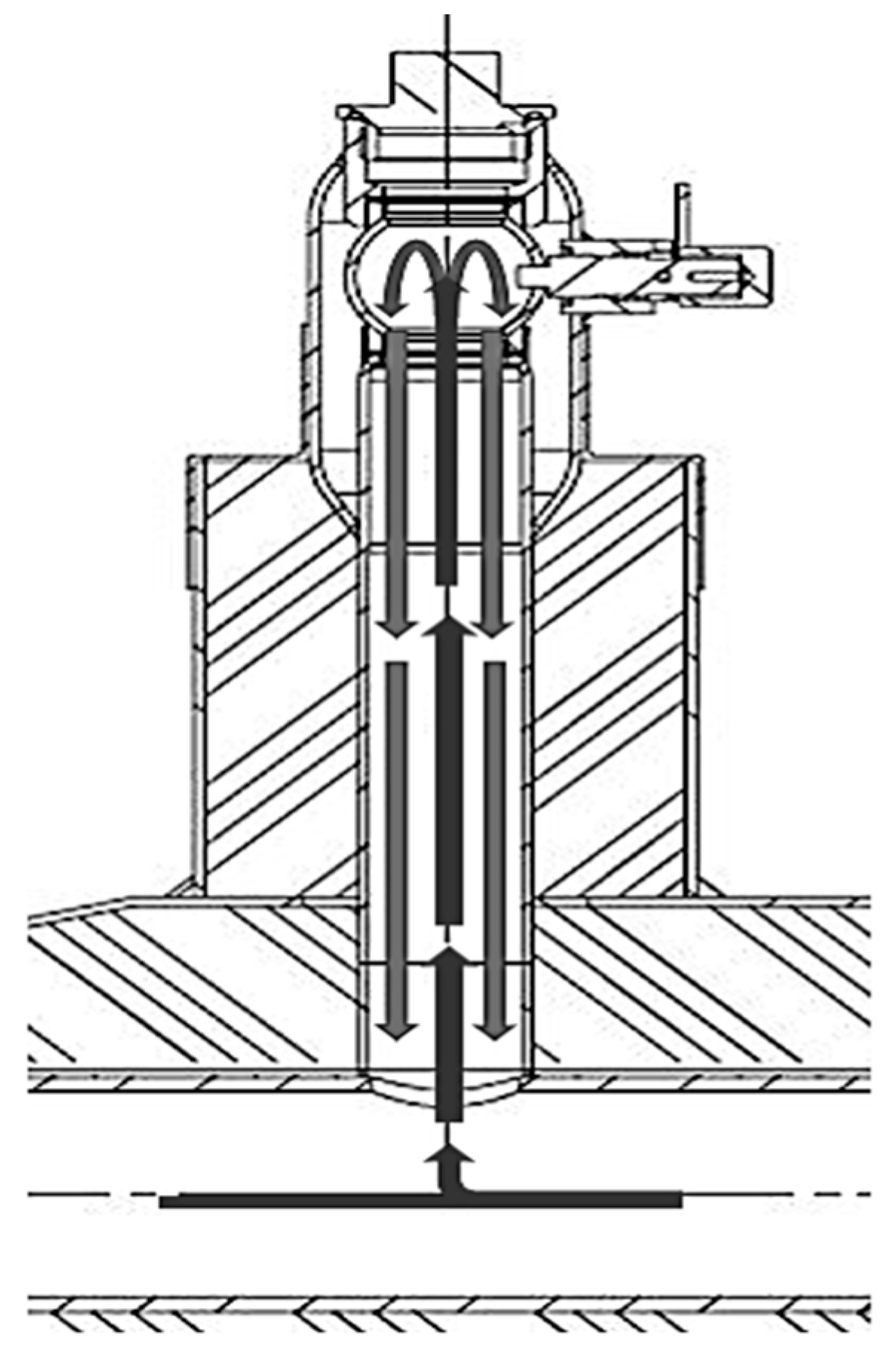
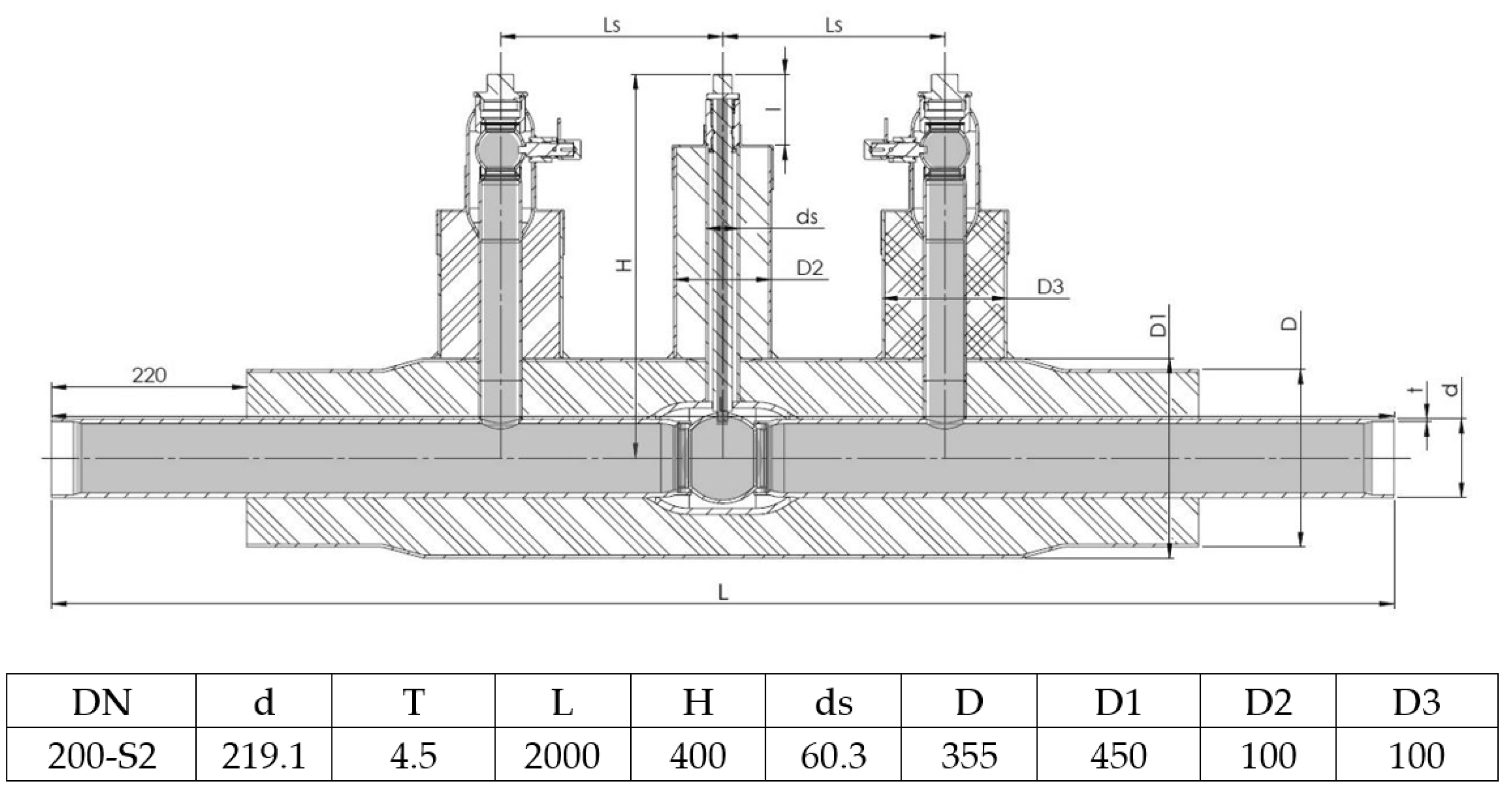
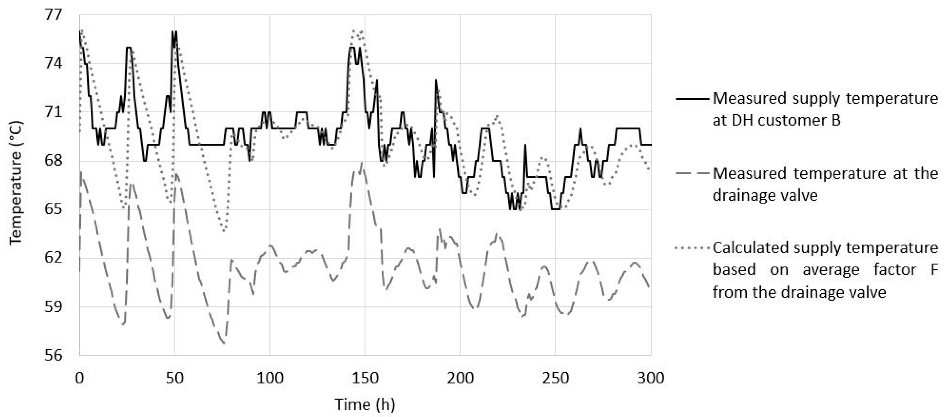
2.2. Measuring Fluid Temperature through Valves

Valves welded to the service pipe permit the measurement of service pipe temperature. These valves are commonly reachable through manholes or culverts. Temperature sensors (thermocouples) can be attached to, for example, drainage valves, which are in direct contact with the medium water, or installed at shutdown valves. The vertical valves reached through a manhole are shown in Figure 6.
Drainage valves contain standing water up to almost the top part. The top part of the shutdown valve (in the centre of the figure) is thermally connected to the water only via the closing ball and its steel rod (stem). The upper parts of the two valve types are uninsulated and directly connected to the air temperature in the manhole. The steel parts of the valves are normally stainless; the material properties of the valves are presented in Table 2.
The valves are insulated with PUR and have a casing made of high-density polyethylene (HDPE).

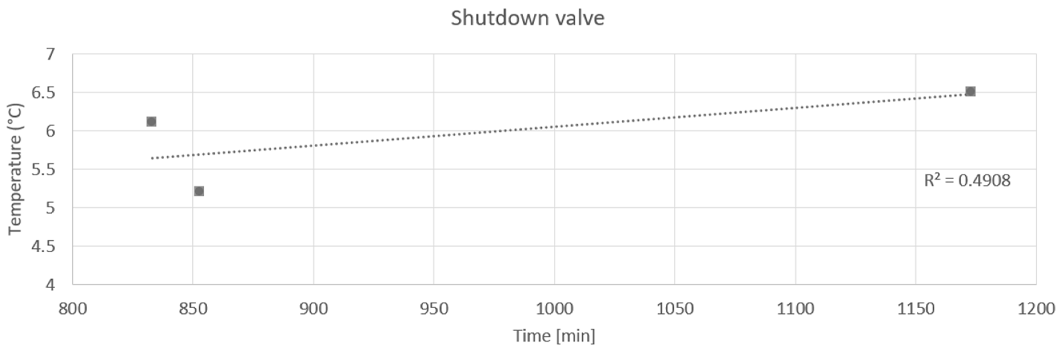
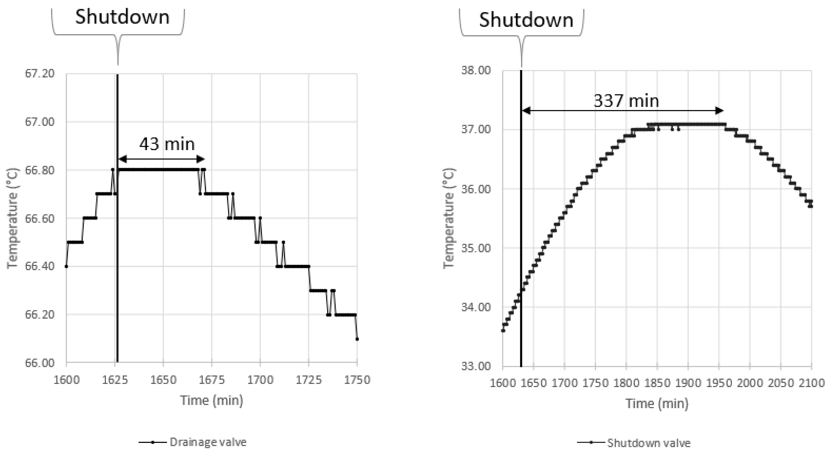
2.2.1. Shutdown Valve

Knowledge of the valves’ thermal response is essential for analysing the decline in the temperature of the water in the supply pipe. In analysing its thermal response, the shutdown valve can be assumed to be a perfectly insulated rod in contact with water in a supply pipe, with no heat losses perpendicular to the direction of the valve. Therefore, one-dimensional heat transfer by conduction is assumed to occur in the steel rod. In a steel rod, the rate of thermal penetration of a sudden change in water temperature in the supply pipe can be calculated using the analytical solution to the heat transfer differential Equation (4). A constant initial temperature, T0, over the whole steel valve is assumed. A sudden temperature change occurs from T0 to T1 at x = 0 at the rod’s connection to the main DH pipe at time zero.
T ( x , t ) = T 0 + ( T 1 T 0 ) e r f c ( x 4 a t )
where a is the thermal diffusivity (m2/s) and t is time (s).
To find out when a certain possible temperature change has occurred at a given position along the steel rod, Equation (5) is used. The depth at which 50% of the temperature change is reached, i.e., the temperature has reached (T0 + T1)/2, is calculated by:
t d 2 a
The temperature response versus depth of a steel rod for various times is presented in Figure 5. The thermal diffusivity of the stainless-steel material is set to 4.1 × 10⁻⁶ (m2/s) (see Table 1).
The results presented in Figure 7 indicate that, after 0.5 h, the heat front has reached 0.35 m into the material; however, this represents a small proportion, less than 1%, of the total possible temperature change. It takes 8 h for half the possible temperature change to occur at approximately the same depth (see the black dot).

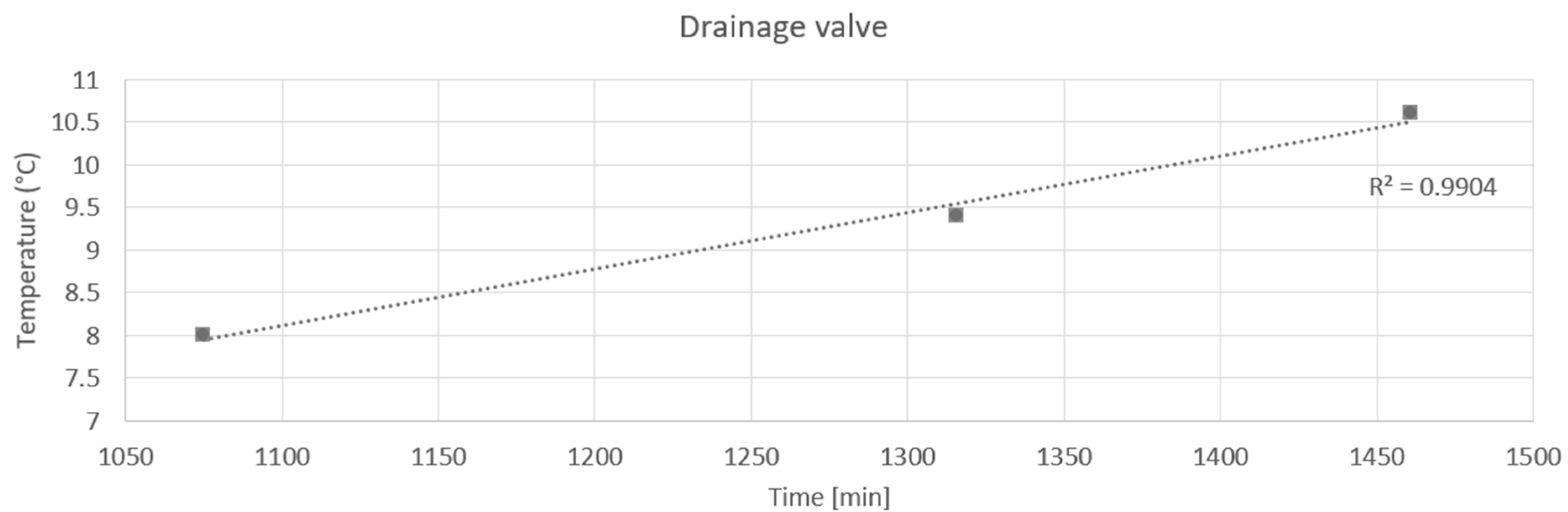
2.2.2. Drainage Valve

The thermal behaviour of the drainage valve is complex since it contains a volume of water, and the temperature difference is enough to induce convective heat transfer in this water. Convective movements are expected to flow upwards in the centre of the valve and down along the side, due to the cooling from the uninsulated top part (see Figure 8).
A shorter thermal response time is expected, due to heat transfer by convection, than in the shutdown valve. Thus, using a drainage valve for assessing a network makes it possible to reduce the shutdown time.

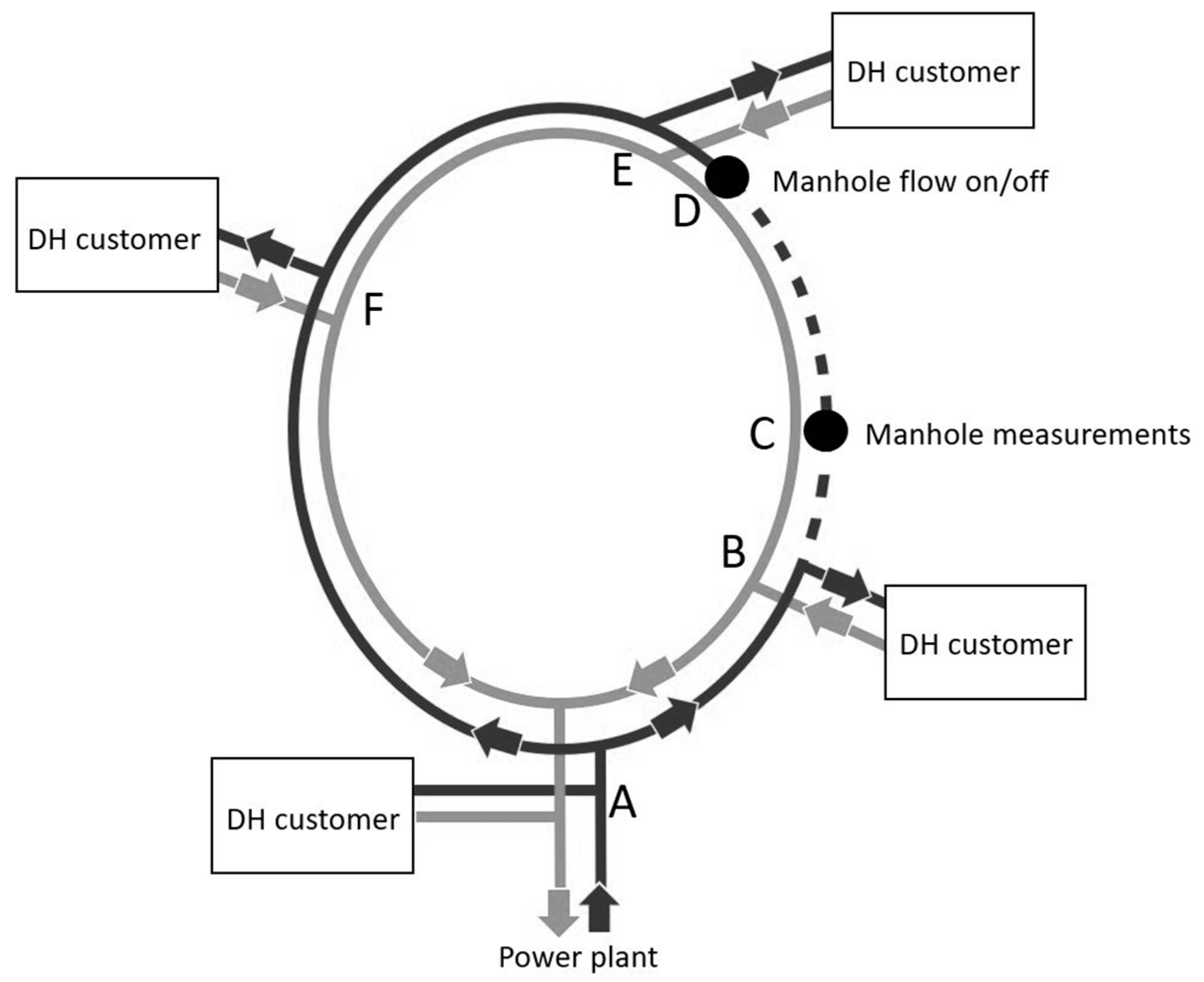
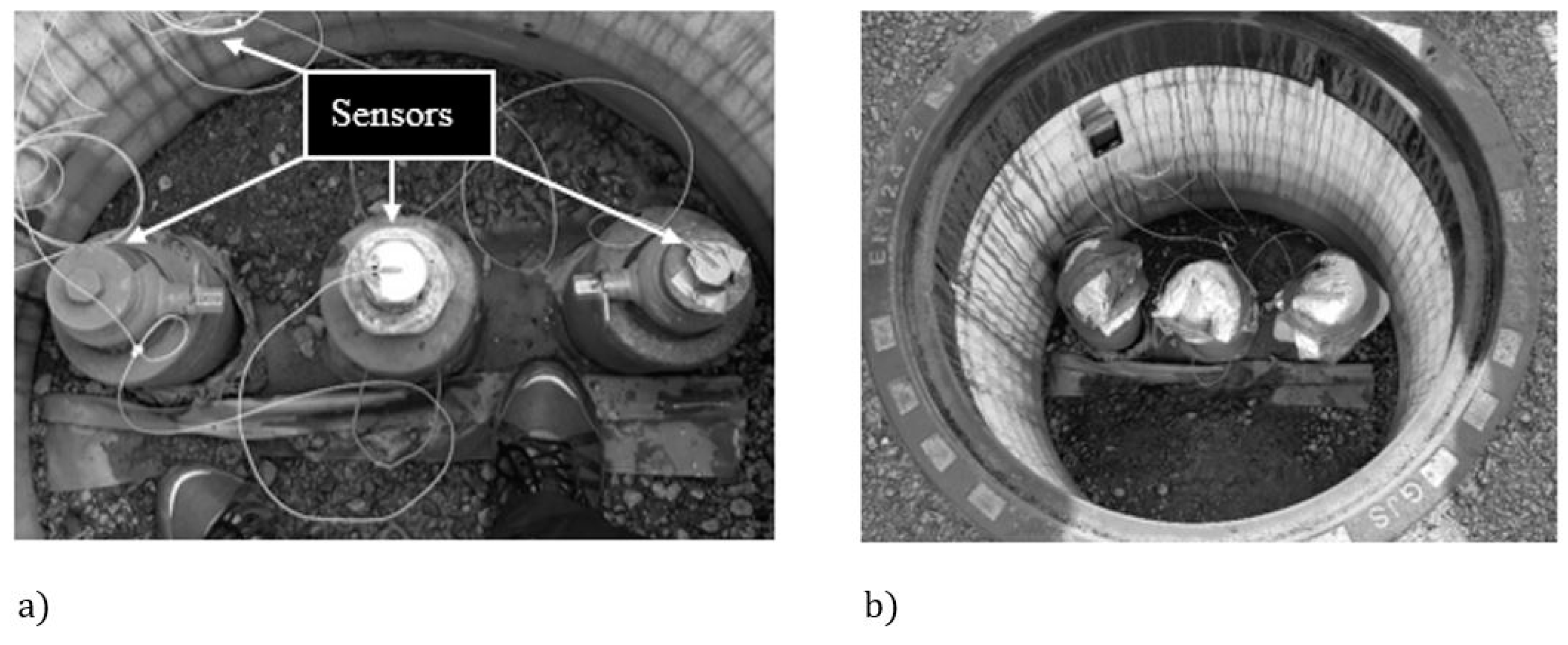
3. Field Measurement of a DH Network

The cooling method was implemented in selected parts of Borås Energy’s DH network. Three shutdowns were performed in May 2020. The measurements were made in a newly installed and operating supply pipe network consisting of a DN200 pipe, i.e., a 219 mm diameter steel supply pipe in a 355 mm diameter casing pipe. The studied part of the DH network (i.e., measurement points B–D, 900 m) is presented in Figure 9; the normal flow direction is from A to D. The DH network shown in Figure 9 is the end circle of a newly installed network branch dimensioned for future customer connections to the network. Furthermore, the circular configuration allows the flow to change direction depending on the demand from DH customers; this always results in the flows meeting at a location that can shift within this circle depending on customer demand. The temperature measurements in the field tests were performed using fiberglass type-K thermocouple sensors, range 0 °C to +400 °C, accuracy ± 0.4 °C, diameter 0.2 mm, while a Testo 176 T4 logger was used for data acquisition.
Thermocouple positions are shown in Figure 10a: one on the steel top of the right drainage valve, one on top of the central shutdown valve, and one on the side of the steel top of the left drainage valve. In addition, one thermocouple was placed on the side of the manhole to capture the surrounding air temperature. After attachment of the thermocouples, “hats” of 20-mm mineral wool were placed to cover the top part of the valves (see Figure 10b).
The network part under assessment extends from points B to D. Measurement data from the field test are shown in Figure 11, together with the three shutdowns and openings of the supply water, marked “off” and “on”, respectively. Furthermore, the supply pipe temperature was measured by the energy company [16] at several nearby customers, with B being of greatest interest as it was closest (400 m) to the measurement point, manhole C (see Figure 9).
It should be noted that the flow takes another path between the DH customers during shutdown, so only the supply temperature between openings and closures is of interest. The results presented in Figure 11 show that the valve responses to shutdowns differ between the drainage valves and the shutdown valve. Sharper temperature changes can be seen for the drainage valves, while the shutdown valve indicates smoother changes, more in line with the manhole temperature. Furthermore, the manhole temperature also varies with shutdowns as well as being influenced by daily changes in air temperature.

4. Analysis of Valve Measurements

Three parameters should be analysed to assess the usability of the valves as measurement points: the absolute temperature in the supply pipe versus the absolute temperature in the valves, the thermal response time from the shutdown in the supply pipe to an actual temperature decline in the valves, and the temperature decline in the valves.

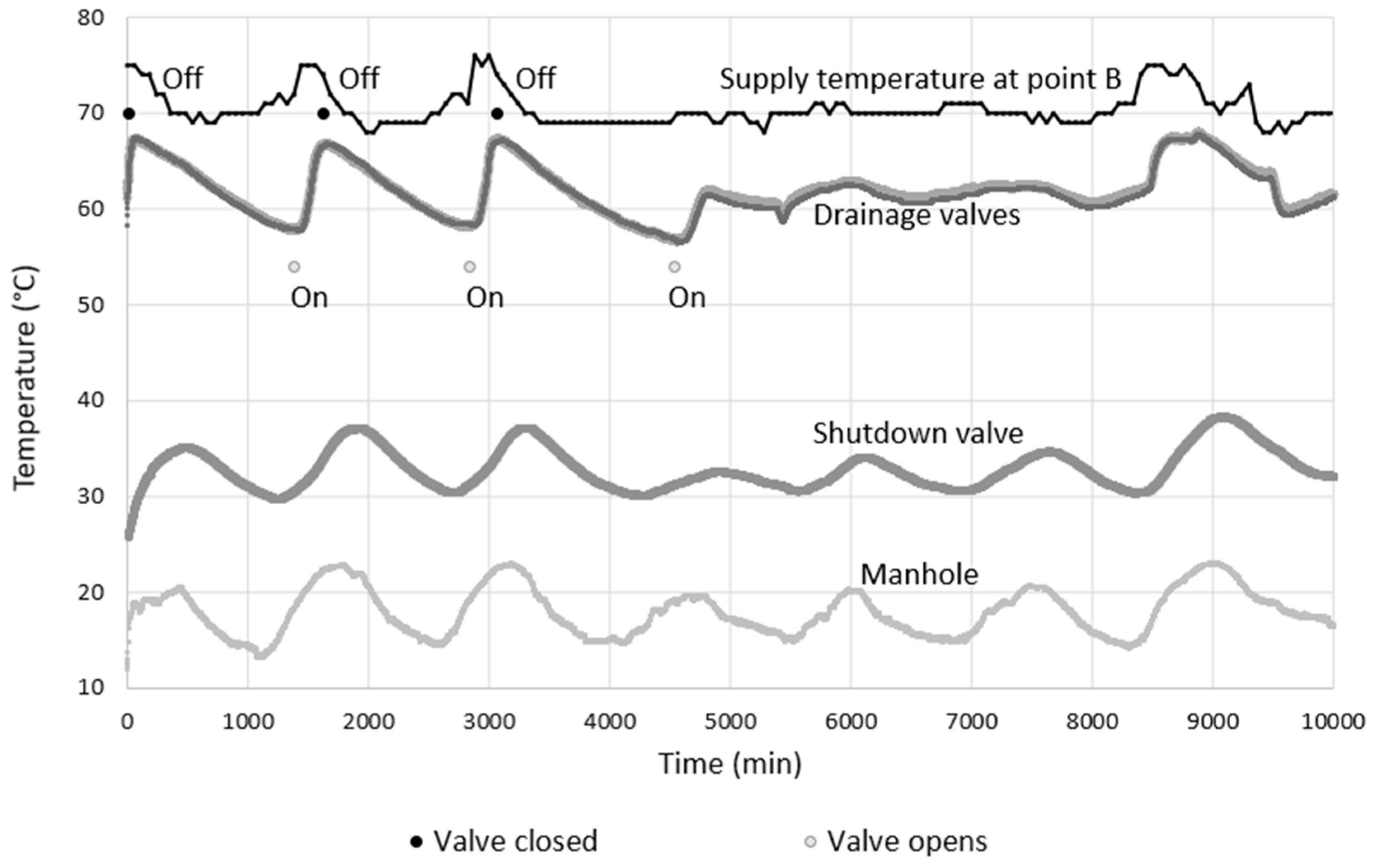
4.1. Absolute Temperature

To assess the interaction and temperature difference between the supply pipe and valves during an operating period without shutdowns, supply temperature data collected at point B are compared with the temperatures measured on the valves. The absolute valve temperature and how it was influenced by the supply and manhole temperatures can be described using a matching factor. However, prior to the assessment, the supply temperature had to be adjusted for time delay due to the 400 m difference in location. This time delay can be seen during normal operation, by comparing the black and grey curves in Figure 11: for example, note the temperature increases after 8000 min, i.e., at 8300 min for the supply and at 8500 min for the drainage valve. This time delay illustrates both the flow velocity of the DH water over 400 m and the thermal response time within the valve material. The flow is approximately 0.1 m/s, which can be considered very low, although the circular network design and the few customers connected so far mainly explain this low flow. When the supply temperatures, Tf, and valve temperatures, Tv, are matched in time, a matching factor, F, can be calculated to illustrate how well the temperatures measured on the valves correlate with the actual supply temperature in the DH pipe. F is calculated according to Equations (6) and (7). A factor of zero indicates a perfect match with the supply temperature and no impact of manhole temperature, Tm; likewise, a factor closer to one indicates an undesirably poor match with the supply temperature:
T v = T f + F ( T m T f )
F = ( T v T f ) / ( T m T f )
The results presented in Table 3 indicate that the drainage valve temperature matches the supply temperature much better than does the shutdown valve temperature. However, the drainage valve and shutdown valve sensors were equally insulated, meaning that the design and material properties of the different valves have a great impact on the resulting temperatures. The supply temperature in the DH pipe below the valves can now be calculated using factor F. In Figure 12, the drainage valve measurement and its factor have been used to calculate the supply temperature. Results show that the deviation between measured and calculated supply temperature is approximately 1%.
Due to the thermal response time of the valve, to be analysed in the next section, a small time lag can be seen in Figure 12 between the measured supply temperature and the measured drainage valve as well as calculated supply temperatures. The matching is very good after the measurement period (after the shutdowns, starting at 80 h). The time delay due to distance between measurement points B and C has been taken into account.

4.2. Thermal Response Time of Valve Material

The resulting matching factors indicate a large difference in heat transfer throughout the two valve types, as can be seen in terms of both absolute temperature and thermal response time.
From Figure 13 it can be seen that the thermal response time is faster in the drainage valve (43 min) than in the shutdown valve (337 min) during the second shutdown. Similar results are observed for shutdowns 1 and 3, where the response times for the drainage valve are 70 and 33 min, respectively, and for the shutdown valve are 510 and 270 min, respectively. The faster response time in the drainage valve is thought to derive from convective water movement within the drainage valve, which constantly supplies the upper part of the valve with hot water from below at a temperature close to the supply pipe temperature. Without the convective heat transfer, the high absolute temperatures cannot be explained. The low thermal conductivity of water in comparison with stainless steel would in that case result in a smaller temperature change than that of the shutdown valve. The shutdown valve’s longer thermal response time is reasonable and can be confirmed by the calculations based on the error function (see Figure 7). Results from the shutdown valve suggest that the manhole temperature has a greater impact on the resulting temperature than does the supply temperature, as also captured by the matching factor.

4.3. Temperature Decline during Shutdown

The measured temperatures of the drainage and shutdown valves during shutdown are presented in Figure 11. A closer look at the temperature decline phases during the shutdowns for the drainage valve reveals a linear temperature decline with time (see Table 4 and Figure 14).
The thermal behaviour of the shutdown valve cannot be assumed to be linear, indicating the great influence of other temperature factors, such as the manhole temperature. The first shutdown has a lower temperature difference than does the second shutdown, even though its duration is longer (see Table 5 and Figure 15). Furthermore, the shutdown period is difficult to distinguish in Figure 11 due to the long thermal response time of the stainless-steel shutdown valve, and also due to the strong interaction with the manhole temperature.
With the present field test set-up, the drainage valve measurements could be used to capture the temperature decline throughout the pipe section (i.e., B–D). However, with the present set-up, the shutdown valve measurements are too complex and unreliable for further thermal assessment of the DH pipe status.

5. Conclusions

The cooling method has been developed through field measurements of a network in operation. Shutting down part of the network resulted in a temperature decline, which could be captured with high accuracy by measuring the temperature decline at a drainage valve. The method was tested during three shutdowns, and the results for the drainage valve indicated little deviation between the tests. The supply temperature data were collected from nearby DH customers during normal operation. The supply temperature was calculated through analysis from valve measurements. The calculated supply temperature agreed well with the measured supply temperature at nearby DH customers. Furthermore, the thermal response time of the valve material was evaluated, and the repeated short response times of the drainage valve constituted a prerequisite for it to serve as a measurement point. The shutdown valve measurements were greatly affected by the manhole environment in the present field test set-up. However, this effect was not seen in the drainage valves, so measurements there were assessed to be usable for further predicting the thermal status of the pipe network. The usage of the shutdown valve should not be dismissed entirely, although an alternative and improved set-up would be required.

Author Contributions

Conceptualization, P.L. and B.A.-Z.; methodology, P.L.; software, P.L.; validation, P.L., B.A.-Z. and C.-E.H.; formal analysis, P.L.; investigation, P.L.; data curation, P.L.; writing—original draft preparation, P.L.; writing—review and editing, B.A.-Z. and C.-E.H.; visualization, P.L.; supervision, B.A.-Z. and C.-E.H.; project administration, P.L. All authors have read and agreed to the published version of the manuscript.

Funding

This research received no external funding.

Conflicts of Interest

The authors declare no conflict of interest.

References

  1. Fredriksen, S.; Werner, S. District Heating and Cooling, 1st ed.; Studentliteratur AB: Lund, Sweden, 2013. [Google Scholar]
  2. Berge, A.; Adl-Zarrabi, B.; Hagentoft, C.-E. Assessing the Thermal Performance of District Heating Twin Pipes with Vacuum Insulation Panels. Energy Procedia 2015, 78, 382–387. [Google Scholar] [CrossRef] [Green Version]
  3. Kręcielewska, E.; Menard, D. Thermal conductivity coefficient of PUR insulation material from pre-insulated pipes after real operation on district heating networks and after artificial ageing process in heat chamber. In Proceedings of the 14th International Symposium on District Heating and Cooling, Stockholm, Sweden, 7–9 September 2014. [Google Scholar]
  4. Kakavand, A.; Adl-Zarrabi, B. Introduction of Possible Inspection Methods for Evaluating Thermal Aging Status of Existing Pre-Insulated District Heating Systems; Chalmers University of Technology: Gothenburg, Sweden, 2015. [Google Scholar]
  5. Lidén, H.P.; Adl-Zarrabi, B. Non destructive methods of district heating pipes. In Proceedings of the 12th European Conference on Non-Destructive Testing (ECNDT 2018), Gothenburg, Sweden, 11–15 June 2018. [Google Scholar]
  6. Lidén, H.P.; Adl-Zarrabi, B. Development of a Non-destructive Testing Method for Assessing Thermal Status of District Heating Pipes. J. Nondestruct. Eval. 2020, 39, 22. [Google Scholar] [CrossRef] [Green Version]
  7. Lidén, P.; Adl-Zarrabi, B. Non-destructive methods for assessment of district heating pipes: A pre study for selection of proper method. In Proceedings of the 15th International Symposium on District Heating and Cooling, Seoul, Korea, 4–7 September 2016. [Google Scholar]
  8. Lidén, P. Development of a Non-Destructive Testing Method for Thermal Assessment of a District Heating Network; Department of Architecture and Civil Engineering, Chalmers University of Technology: Gothenburg, Sweden, 2020. [Google Scholar]
  9. Hagentoft, C.E. Heat loss to the ground from a building. Slab on the ground and cellar, LTH/TVBH-1004. In Building Physics; Building Physics: Lund, Sweden, 1998. [Google Scholar]
  10. Bilskie, J. Dual Probe Methods for Determining Soil Thermal Properties, Numerical and Laboratory Study. Ph.D. Thesis, Iowa State University, Ames, IA, USA, 1994. [Google Scholar]
  11. Broen. District Heating Product Catalogue 2021. 2021. Available online: www.Broen.com (accessed on 5 May 2021).
  12. Powerpipe. Product Catalog. 2018. Available online: www.Powerpipe.se (accessed on 4 February 2021).
  13. Stadtwerke Leipzig. Zeitstandsverhalten von PUR-Schäumen in Praxisgealterten Kunststoffmantelrohren Hinsichtlich Wärmedämmung und Festigkeit (Verbundprojekt); Report; 2004; Available online: https://www.tib.eu/de/suchen/id/TIBKAT:477726356/Zeitstandsverhalten-von-PUR-Sch%C3%A4umen-in-praxisgealterten?cHash=87d46170aa884823417ce10077ab42bf (accessed on 4 February 2021). [CrossRef]
  14. Bing. Thermal Insulation Materials Made of Rigid Polyurethane foam (PUR/PIR) Properties—Manufacture; Federation of European Rigid Polyurethane Foam Assosiation: Brussels, Belgium, 2006. [Google Scholar]
  15. Matmatch. 2020. Available online: Matmatch.com (accessed on 5 January 2020).
  16. Fjellborg, F. Data Received from Energy Company; Borås Energy: Borås, Sweden, 2020. [Google Scholar]
Figure 1. Quasi-steady-state thermal process in the insulated district heating (DH) pipe. The fluid temperature before time zero, i.e., the time of shutdown, is denoted T f 0 (K); the corresponding temperature in the surrounding insulation is denoted T i ( r , t = 0 ) (K), while the immediately surrounding soil temperature is T s ,   s . The heat loss is q f , s (W/m).
Energies 14 05192 g001
Figure 2. (a) total transient thermal process, (b,c), superposition of two elementary processes, to analyse the cooling of the pipe after shutdown.
Energies 14 05192 g002
Figure 3. (a) Expected cooling times for pipes of different dimensions; (b) close-up of expected temperature declines during a shutdown; MATLAB model according to Section 2.1.1, Ts fixed at 10 °C.
Energies 14 05192 g003
Figure 4. Illustration showing the small effect of different soil types on cooling time; MATLAB FDM model.
Energies 14 05192 g004
Figure 5. Illustration of the insignificant effect of recent temperature history in the supply pipe prior to a shutdown; equal temperature declines for the three shutdowns at 61–85 h, 139–163 h, and 291–315 h.
Energies 14 05192 g005
Figure 6. Illustration of valves: an open/close ball valve in the middle and drainage valves to the left and right. The grey shading represents the medium water in a pressurised system (illustration modified from Broen [11]).
Energies 14 05192 g006
Figure 7. Progress of the heat front in a stainless-steel rod for times ranging from 0.5 to 8 h; dashed lines represent how deep into the material half of the possible temperature change has progressed.
Energies 14 05192 g007
Figure 8. Expected convective water movements in a drainage valve.
Energies 14 05192 g008
Figure 9. Pipe network and measurement location C (i.e., valves). Normal flow direction is A–E. During shutdown at valve point D, the flow between B and D (dashed line) stops. Supply water is shown in black and return water in grey.
Energies 14 05192 g009
Figure 10. (a) Measurement set-up in the manhole, showing thermocouples attached to the three valves and one to the side of the manhole to capture the air temperature; (b) the valves insulated with mineral wool (the valve set-up is the same as in Figure 6).
Energies 14 05192 g010
Figure 11. Temperature measurements during the three shutdowns (i.e., off to on) followed by normal operation starting at approximately 4500 min.
Energies 14 05192 g011
Figure 12. Calculated supply temperature in the DH pipe based on factor F for the drainage valve.
Energies 14 05192 g012
Figure 13. Thermal response time from shutdown to temperature decline for the drainage valve (left panel) and shutdown valve (right panel); temperature data from the second shutdown, at 1627 min.
Energies 14 05192 g013
Figure 14. Three shutdowns showing temperature difference versus duration of temperature decline for the drainage valve.
Energies 14 05192 g014
Figure 15. Three shutdowns showing temperature difference versus duration of temperature decline for the shutdown valve.
Energies 14 05192 g015
Table 1. Soil properties [10].
Soil TypeWater Content (m3/m3)Thermal Conductivity (W/mK)Volumetric Heat Capacity (106 J/ m3K)
Loam0.2951.012.16
Sand dry0.0221.531.36
Sand wet0.3513.082.68
Table 2. Material properties of polyurethane (PUR) [12,13,14], high-density polyethylene (HDPE) [15], and carbon and stainless steels used in DH networks [15]. Thermal diffusivity is calculated from the table values.
DH ComponentDensity (kg/m3) at 20 °CThermal Conductivity (W/mK) at 20 °CSpecific Heat Capacity (J/kgK) at 20 °CThermal Diffusivity (m2/s) at 20 °C
HDPE casing9500.38–0.512100–27001.97 · 10−7
PUR insulation61 *0.026 *1400–15002.31 · 10−7
Mineral wool insulation1300.368400.22 · 10−7
DH water9980.6042001.40 · 10−7
P235GH **785057.54601.59 · 10−5
P235TR1/P235TR2 **785056.94601.57 · 10−5
AISI 304 ***780016.05004.10 · 10−6
* New pipes [12], ** Carbon steel, *** Stainless steel used in drainage and shutdown valves.
Table 3. Calculated average matching factors for the two valve types, with their standard deviations and coefficients of variation.
Drainage ValveShutdown Valve
Factor (F)0.150.71
Standard deviation0.020.28
Coefficient of variation13.5%39.0%
Table 4. The three shutdowns with thermal response times to the temperature declines, and temperatures at one of the drainage valves.
Thermal Response Time (min)Temperature Decline, Duration (min)Temperature, MAX (°C)Temperature, MIN (°C)Temperature Difference (°C)Temperature Decline (°C/h)
First shutdown70131667.458.09.40.43
Second shutdown43107566.858.48.00.45
Third shutdown33146167.256.510.60.44
Table 5. The three shutdowns with thermal response times to temperature declines, and temperatures at the shutdown valve.
Thermal Response time(min)Temperature Decline, Duration (min)Temperature, MAX (°C)Temperature, MIN (°C)Temperature Difference (°C)Temperature Decline (°C/h)
First shutdown51085335.129.95.20.37
Second shutdown33783336.730.66.10.44
Third shutdown270117336.730.26.50.33
Publisher’s Note: MDPI stays neutral with regard to jurisdictional claims in published maps and institutional affiliations.

