Article

Diagnostic Protocol for Thermal Performance of District Heating Pipes in Operation. Part 2: Estimation of Present Thermal Conductivity in Aged Pipe Insulation

Department of Architecture and Civil Engineering, Chalmers University of Technology, 412 96 Gothenburg, Sweden
*
Author to whom correspondence should be addressed.
Energies 2021, 14(17), 5302; https://doi.org/10.3390/en14175302
Submission received: 18 July 2021 / Revised: 16 August 2021 / Accepted: 24 August 2021 / Published: 26 August 2021
(This article belongs to the Special Issue Recent Advances in District Heating)

Abstract

:
Buried and operating district heating (DH) pipes are exposed to thermal degradation of their polyurethane (PUR) insulation over time, and their status is hard to assess without excavation. By using DH pipe valves in manholes as measurement points during a shutdown with an ensuing cooling period, non-destructive assessments can be performed. This study compares new improved field measurements with numerical simulations of the temperature decline in drainage valves and shutdown valves. The drainage valve measurements were used to thermally assess part of a buried DH network. Results indicate that by using the drainage valves as measurement points in a cooling method, the thermal conductivity of the buried DH network could be predicted with an accuracy of >95%. In addition, a general diagnostic protocol has been established for assessing the thermal status of a DH network, ready for network owners to use.

1. Introduction

District heating (DH) networks are widely used in urban areas throughout the world, and their usage, which started to expand greatly in the 1960s in the USA and Europe, has evolved in large networks of varying age. A typical rigid DH pipe in a Swedish DH network consists of an inner service pipe of steel and an outer casing pipe of polyethylene (PE). As an insulation layer, polyurethane (PUR) foam is inserted between the inner steel pipe and the outer casing pipe [1]. Through aging and degradation, the PUR foam loses its insulating capacity with time, resulting in unwanted heat losses [2]. Numerical modelling has been conducted for the assessment of heat losses in DH pipes, e.g., [3,4,5,6]. However, we lack an on-site method in field for quantifying these heat losses, which are hard to assess with high accuracy for isolated parts of a network, especially in a non-destructive manner in an operating network.
A “cooling method” was previously developed by the authors for use during network maintenance with an excavated pit [7,8,9]. This cooling method requires the temporary shutdown of part of the pipe network, while the ensuing cooling process is registered by thermocouples that capture the temperature decline in the supply pipe. The thermal status of the pipe network can then be calculated using the measured temperature decline of the supply pipe. While the method was usable for pipes during maintenance with excavation, it was further developed to allow assessment of a pipe network in operation, without excavation. The method was implemented as the evaluation of indirect temperature measurements using sensors installed at drainage and shutdown valves, insulated with 20 mm of mineral wool, in manholes [10]. The evaluation concluded that the drainage valves could be used to capture the temperature decline in the pipe network with high accuracy, and that the results might be usable for predicting the thermal status of the pipe network using a numerical finite difference method (FDM). However, the study also showed that, with the used measurement set-up, temperature measurements made on the shutdown valve had a limited ability to capture the temperature decline.
The purpose of this paper is to evaluate how temperature measurements made by thermocouples at the valves could be used in an improved measurement set-up in a field test. The temperature decline at the top of the drainage and shutdown valves in a manhole is analysed analytically and numerically by developing new FDM models in MATLAB for the cooling period for comparison with the field measurements. Furthermore, the thermal status of the DH pipes is assessed by evaluating the thermal conductivity of the PUR insulation. Finally, general suggestions are presented regarding how to perform a thermal status assessment using the present cooling method.

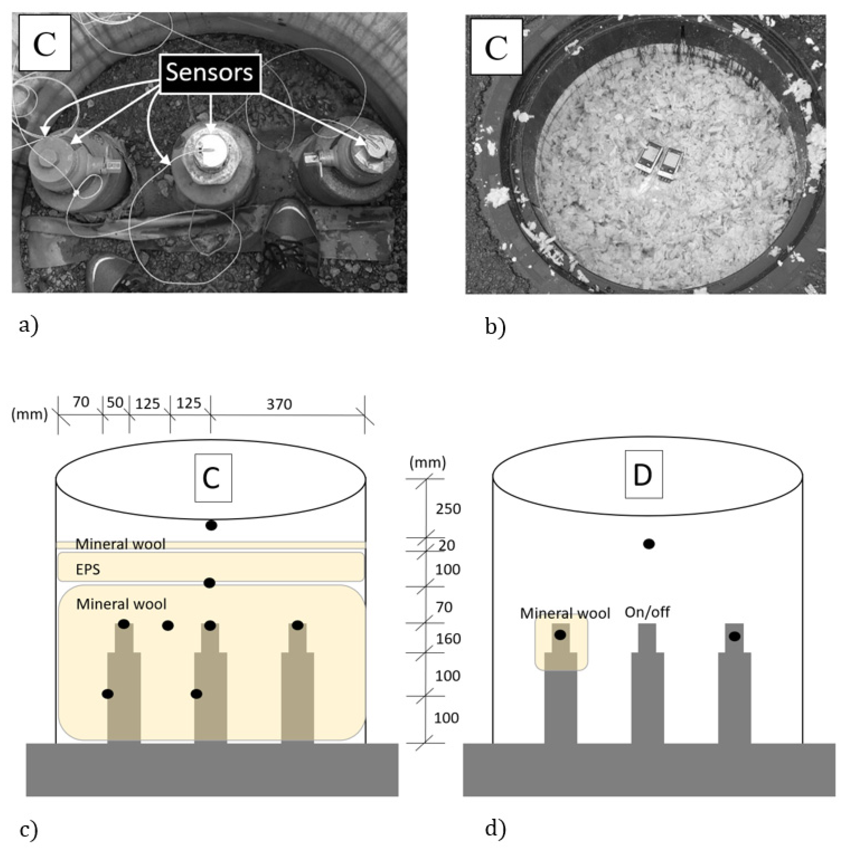
2. Improvements in the New Measurement Set-Up

The cooling method using temperature measurements at valves has been modified and improved to further evaluate the potential for using shutdown valve measurements. As in the previous field tests [10], the same selected parts of Borås Energy’s DH network were used. The improvement consisted of using a mineral-wool–filled manhole and expanded polystyrene insulation board (EPS), in contrast to the previous set-up, which used only an insulating “hat” of 20-mm mineral wool. Furthermore, additional measurements were performed in the manhole where the water flow was turned on and off. Three shutdowns were performed in April 2021. The measurements were made on the newly installed supply pipe network in operation, consisting of DN200 pipe, i.e., 219-mm diameter steel supply pipe within 355-mm diameter casing pipe. The studied part of the DH network (i.e., measurement points B–D, 900 m) is presented in Figure 1; the normal flow direction is A–D. The DH network shown in Figure 1 is the end circle of a newly installed network branch dimensioned for larger connections to the network in the future. Furthermore, the circular configuration allows the flow to change direction depending on the demand from DH customers; this always results in the flows meeting at a location that can shift depending on customer demand. The temperature measurements in the field tests were performed using fiberglass type-K thermocouple sensors, range 0 °C to +400 °C, accuracy ± 0.4 °C, diameter 0.2 mm, while a Testo 176 T4 logger was used for data acquisition.
Inside manhole C, thermocouples were placed on top of the drainage valves to the left and right and on top of the shutdown valve located between the drainage valves (see Figure 2a). Two thermocouples were installed, one on the casing of one drainage valve and one on the casing of the shutdown valve. One thermocouple was placed in the mineral wool between the drainage valve and the shutdown valve, in line with the tops of the valves. One thermocouple was placed below the EPS board and one above all the insulation to capture the surrounding air temperature in the 250-mm free space below the manhole cover (see Figure 2c). Inside manhole D, where the water flow was turned on/off at the shutdown valve, three thermocouples were placed as control points: one at a drainage valve with a 20-mm insulation hat on top, one at a drainage valve without insulation, and one positioned in the free space to capture the air temperature, as in manhole C (see Figure 2d).
The part of the network under assessment extends from points B to D. The temperatures measured in manhole D will be used only as control points during normal operation, since a complex water-flow pattern occurs beyond manhole D during a shutdown (due to low flow between points D and E, colder water influences the shutdown/temperature decline phase).

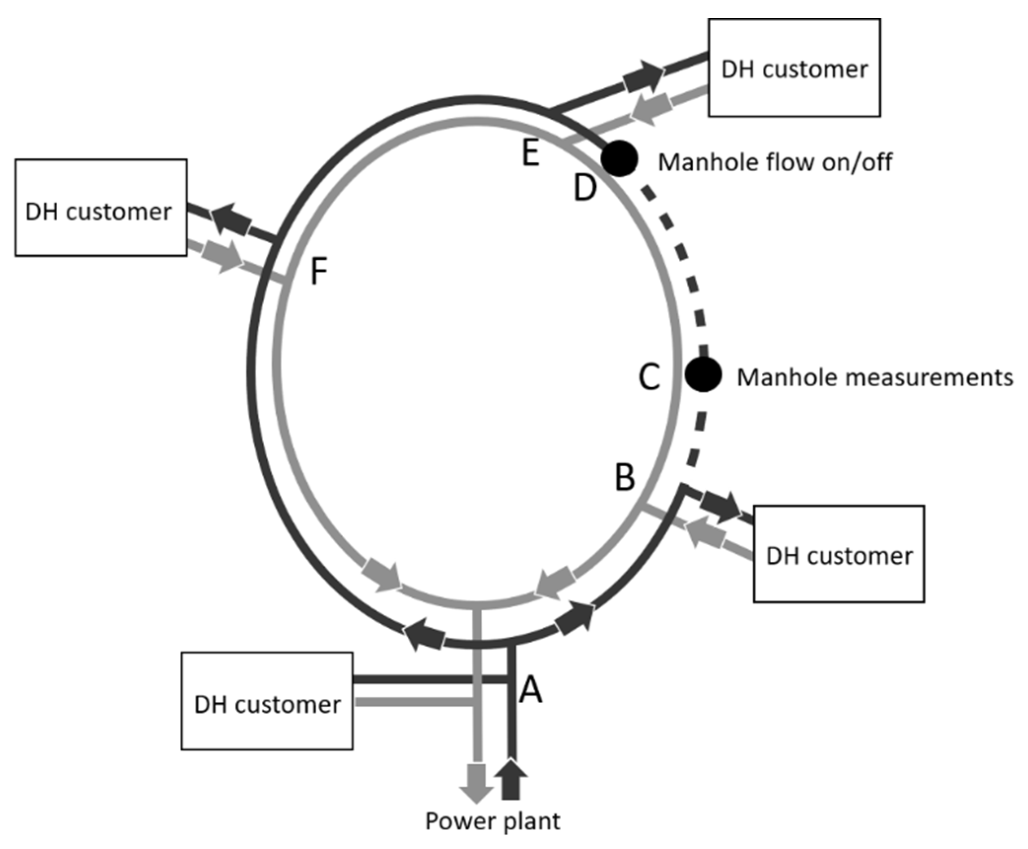
3. Potential Use of Shutdown Valve Measurements

In previous field tests [10] an improved set-up was recommended. The new set-up includes a mineral-wool–filled manhole in order to greatly reduce transverse heat losses from the valves in the manhole and to attain well-insulated surroundings in the manhole.

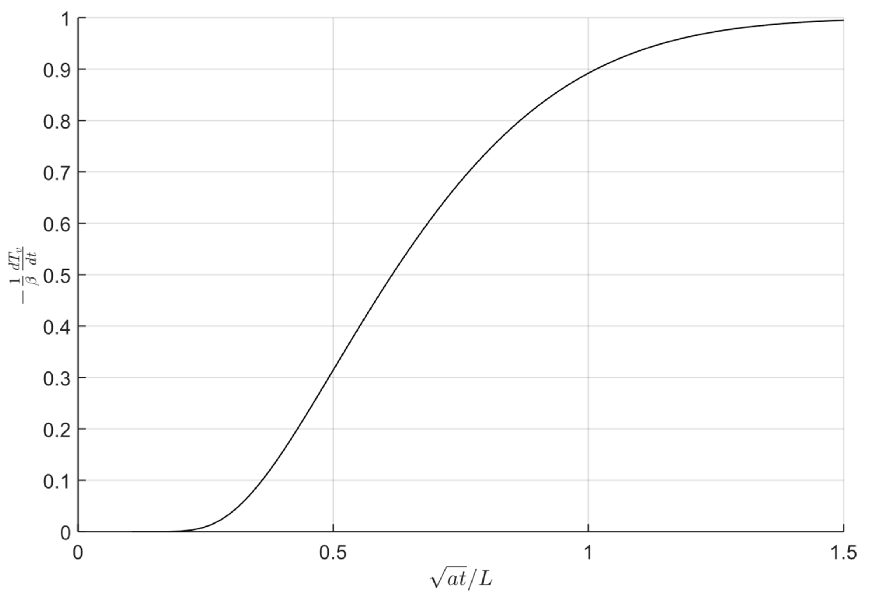
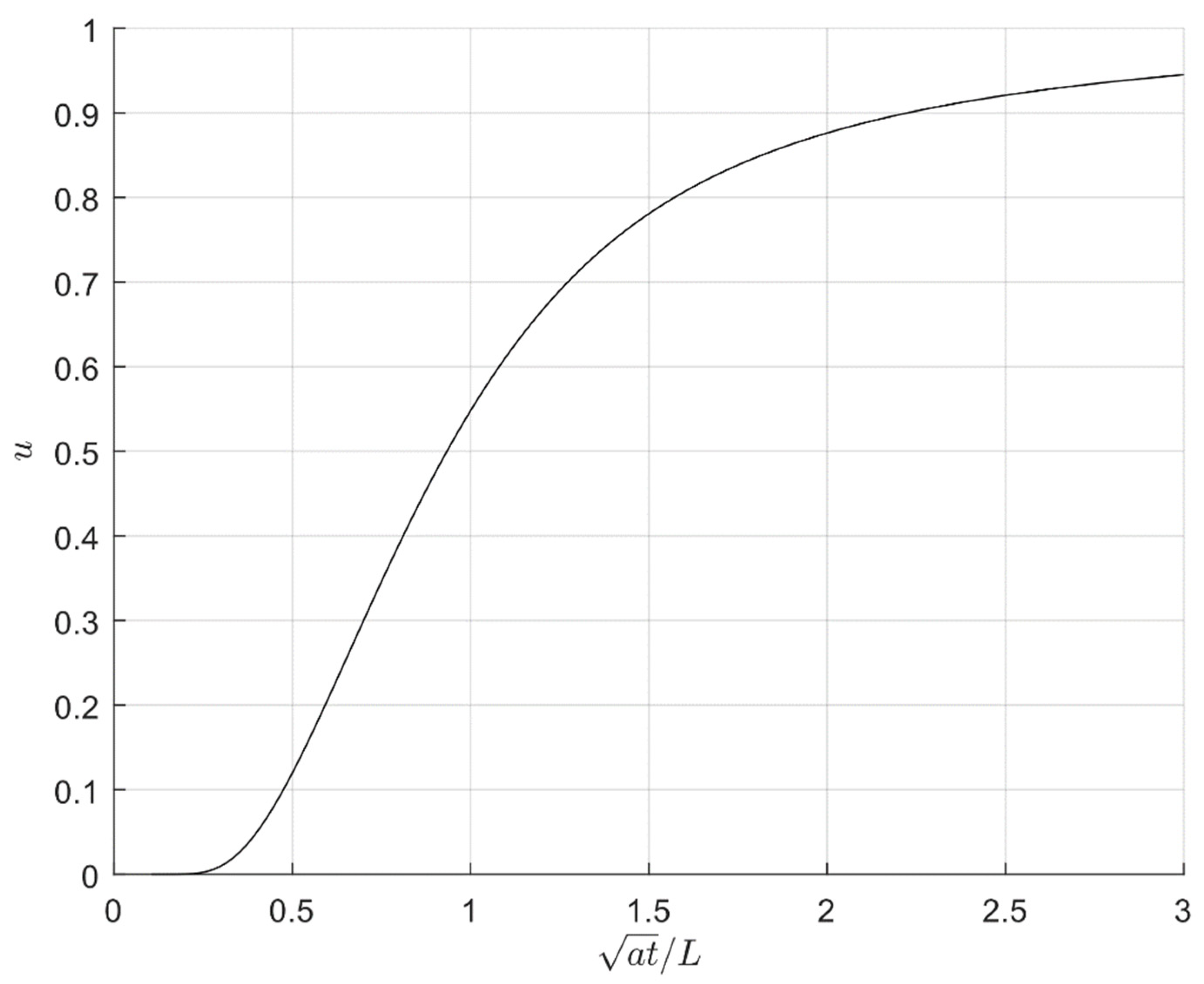
3.1. Mathematical Model of an Optimal Case (No Transverse Heat Losses)

To investigate the possibility of using the shutdown steel valve (rod) in determining the supply pipe temperature, a perfectly insulated shutdown valve is assumed, i.e., no influence from the ambient air of the manhole. Laplace transforms were used for calculating the temperature. These calculations/analyses assume that prior to a shutdown, with previous constant supply temperatures, the temperature at the top of the valve, T v ( 0 ) , equals the supply fluid temperature, T f , for t 0 . The supply pipe temperature is assumed to decline linearly after shutdown, i.e., t > 0.
T f = T v ( 0 ) β t       t > 0
T f = T v ( 0 ) t 0 °
The length of the rod is L (m) and the thermal diffusivity is a (m2/s). β (−) is the temperature decline slope factor. The temperature at the valve sensor T v is:
T v = T v ( 0 ) β t u ( a t L )
Figure 3 shows the non-dimensional parameter. The results shown in Figure 3 indicate that the thermal response time is initially long, and that for long times the temperature increase reaches the temperature in the supply pipe when u = 1. For example, if the temperature drop in the supply pipe is 2 °C after 5 h, then a t L = 0.9 for the same time, u then equals 0.5, indicating that half of the temperature drop has reached the valve sensor, which then is a drop of 1 °C.
Figure 4 shows the slope function 1 β d T v d t , describing the relation between the slope of the supply pipe temperature and the slope of the temperature at the sensor on top of the valve. This slope can then be used to adjust the measured temperature slope at the valve to match the actual slope in the pipe.
This slope relation will be used in comparing the calculated results and the results of field measurements.

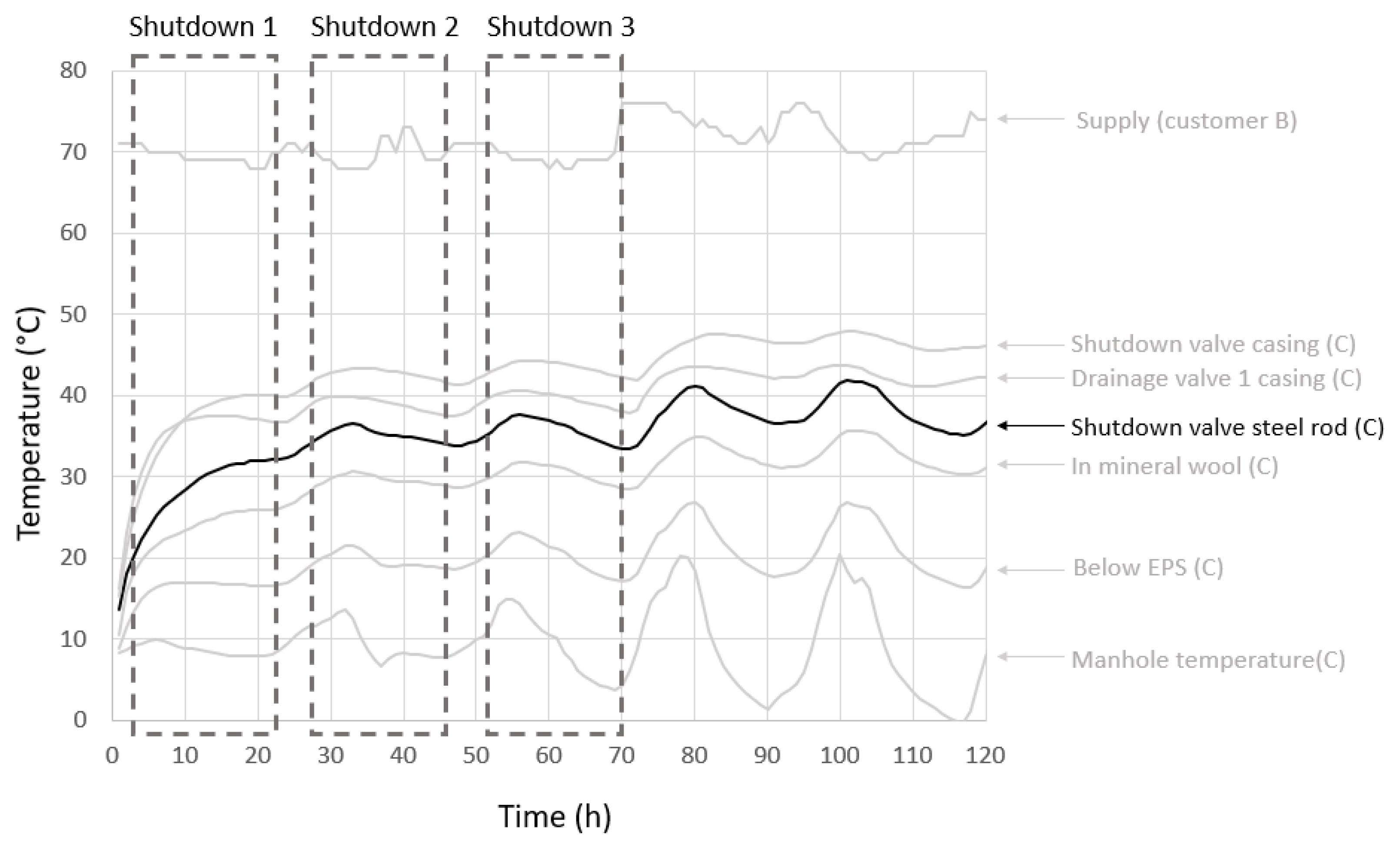
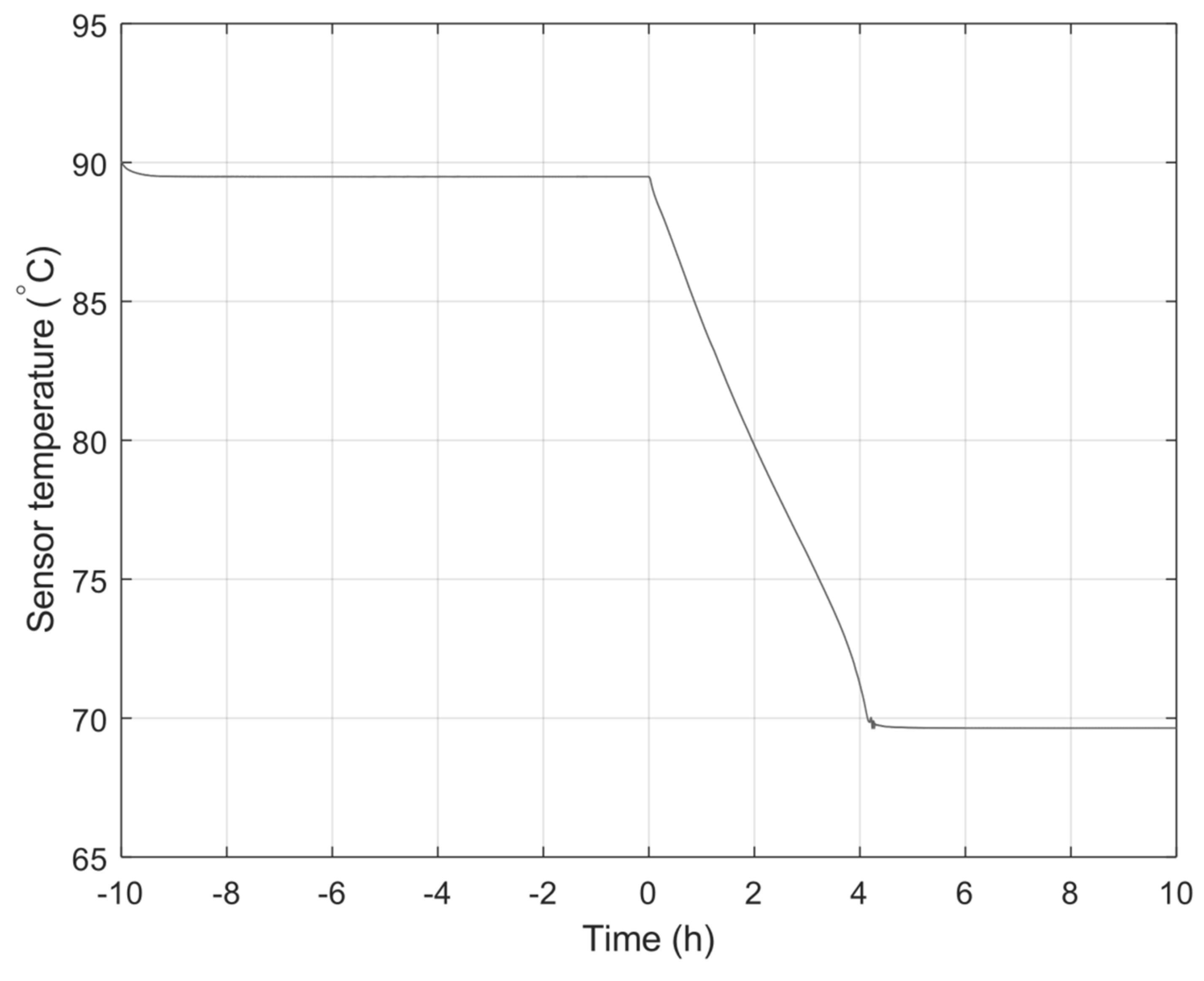
3.2. Results of Field Test Measurements

The whole test period is shown in Figure 5, including all thermocouples with information regarding the shutdown valve. All temperature data are from manhole C, apart from the customer B supply temperature data, which were collected by the energy company [11]. Here B is of most interest among the customers, as it is close (400 m) to the manhole C measurement point (see Figure 1). The accuracy for the measured absolute temperature by the thermocouples is ±0.4 °C for both valves and DH customers, resulting in a total accuracy of ±0.8 °C. The supply temperature in the investigated pipe below the manhole is not equal to the customer B supply temperature during the shutdowns. The period after the shutdowns, from 70 to 120 h, illustrates how the system recovers and continues with its normal fluctuations. The temperature measurements start at time 0, immediately after the insulation is installed in the manhole. The first shutdown starts approximately 4 h later. Results indicate that a long time is required for the thermal adaptation of the thermocouples to their surroundings, so the temperature rises despite the first shutdown having begun. An optimal case would include a longer adaptation period prior to the first shutdown. Therefore, an analysis can be made from shutdowns two and three. The results of this analysis clearly show the effect of the thickness of the additional covering insulation: the coldest temperatures are registered by the thermocouple measuring the air temperature in the manhole just below the cover, whereas the temperatures progressively increase deeper into the manhole. The two thermocouples on the valve casings are the ones in the deepest position and accordingly register the highest temperatures. The shutdown valve casing shows the highest temperature due to its central position, unaffected by the colder manhole wall. The purpose of full insulation was to evaluate whether the influence from the manhole temperature could be reduced enough to perform an accurate analysis of the temperature decline at the shutdown valve. As seen in Figure 5, the air temperature in the top part of the manhole can still be seen to have a dampening effect on all thermocouples, leading to a complex analysis of the temperature decline at the shutdown valve during shutdown. The results from the thermocouple on the shutdown valve and from the one in the mineral wool (see Figure 2) are in line with each other. However, the temperature is approximately 6 °C higher at the shutdown valve than at the thermocouple in the mineral wool, due to conduction via the shutdown valve from the supply pipe. The temperature decline at the shutdown valve in shutdowns two and three starts approximately 5–6 h after the shutdown, as expected due to the thermal response time in the stainless steel rod of the valve [10].
In the present tests, using an insulation “hat” on the shutdown valves was not feasible since one valve was fully insulated (manhole C) and one was used for turning the flow on and off (manhole D). However, results from the fully insulated shutdown valve can now be compared with previous test results obtained using an insulation hat.
The previous paper described a matching factor [10] capturing how well the temperatures measured on the valves correlate with the actual supply temperature in the DH pipe. This factor is now used to compare the new measurement set-up (fully insulated) with the previously used set-up (hat insulated). Factor F is calculated according to Equations (4) and (5). A factor F of 0 indicates a perfect match with the supply fluid temperature, Tf, and no impact from the manhole temperature, Tm. Likewise, a factor closer to 1 indicates an undesirably poor match with the supply temperature.
T v = T f + F ( T m T f )
F = ( T v T f ) / ( T m T f )
The comparison between the previous measurement set-up (hat insulated) and the new set-up (fully insulated) is shown in Table 1. The matching factor decreased between the previous and new set-ups. The shutdown valve, which had an undesirably high factor in previous tests, now has a better factor result, i.e., 0.53 versus 0.71.
In addition to the matching factors, the thermal response time and slope are compared between the previous and present field tests, as shown in Table 2. Slope is the temperature decline, °C/h, measured at the valves. The results for the shutdown valve indicate, as did previous measurements, considerable deviation between the shutdowns.

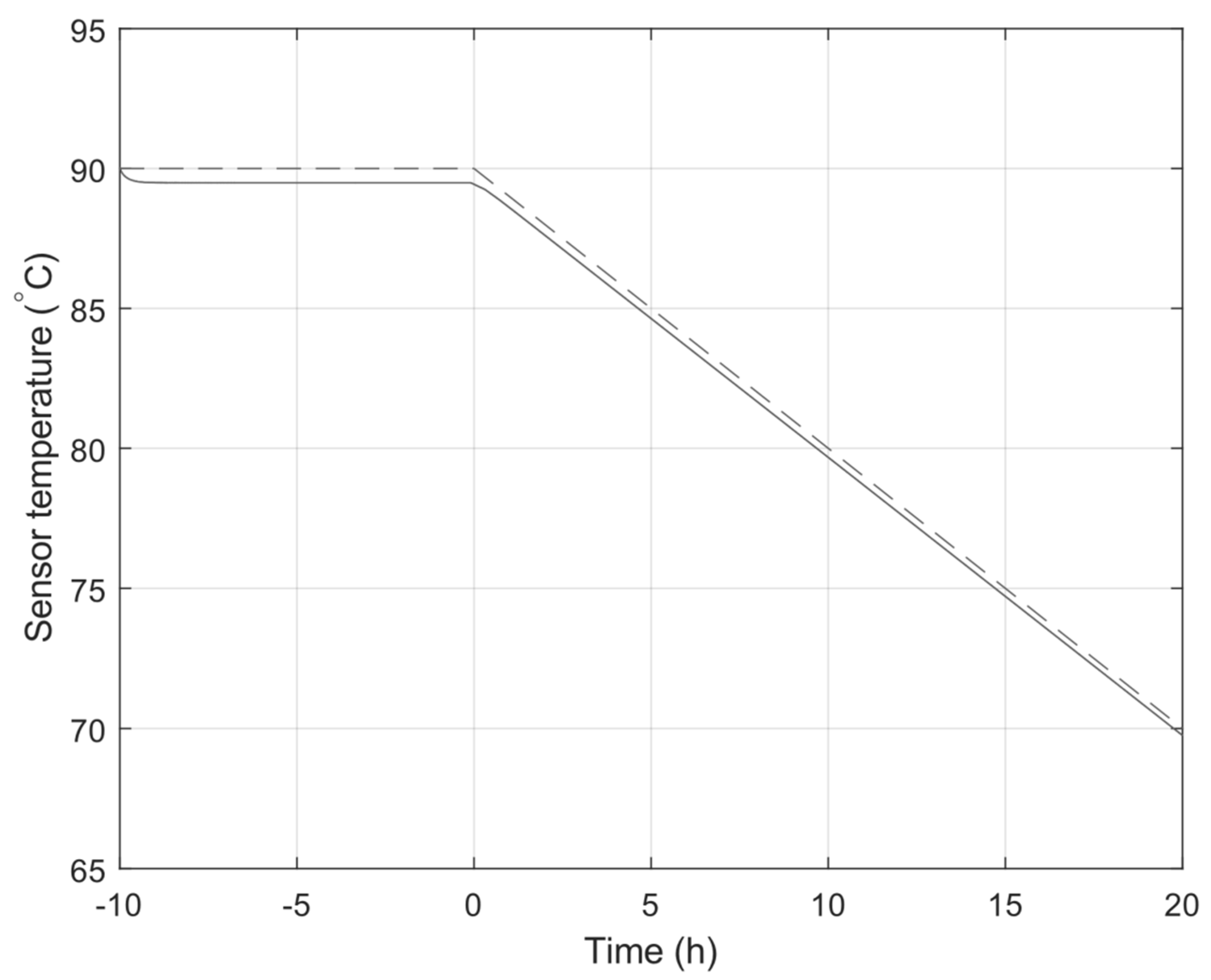
3.3. Simulation Model Compared with Measurements

The measurement results for the shutdown valve indicate a strong influence from the manhole temperature. In an optimal set-up, if the disturbance from the manhole were totally reduced (i.e., a matching factor close to zero), accurate analysis could be performed. All shutdowns captured in previous and present field results give an average slope of 0.32 °C/h throughout the cooling phase after the thermal response time. The optimal slope at the valve compared with the slope in the DH pipe is shown in Figure 4. If the slope measured at the valve is to be comparable to the optimal slope, a specific time needs to be considered, preferably late in the cooling phase for higher accuracy. The measured average slope for the 15th h of the cooling phase, for the five shutdowns, was approximately 0.15 °C/h. According to Figure 4, 15 h gives a slope function for the valve close to 1, i.e., the same slope as in the DH pipe. Numerical simulations by the present authors indicate a temperature decline of approximately 0.45 °C/h in the DH pipe [10], i.e., three times higher than the measured average slope during the 15th h. It can thereby be concluded that the long thermal response time together with the great influence of the manhole temperature do not allow for accurate assessment. Hence, the shutdown valve must be dismissed as a potential measurement point.

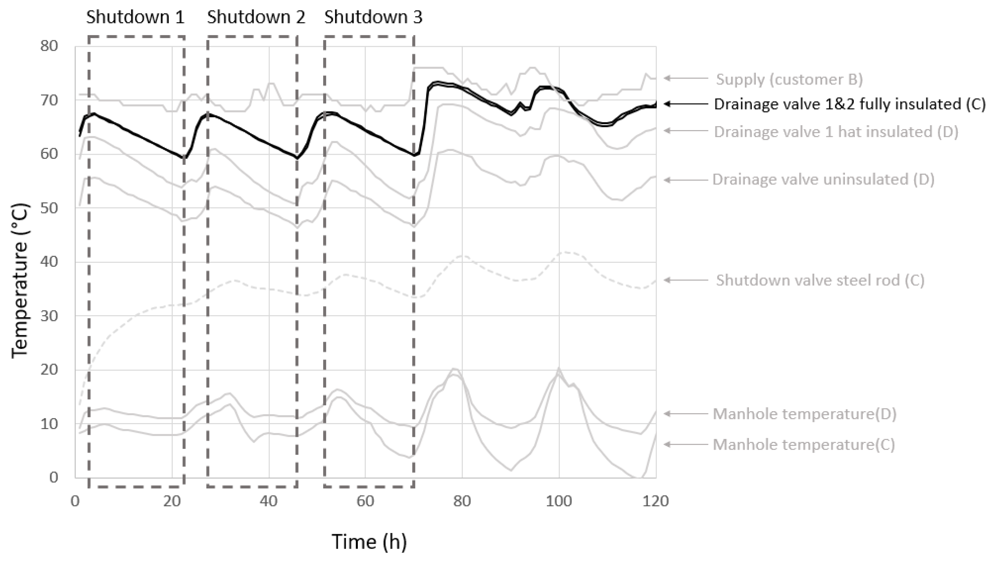
4. Potential Use of Drainage Valve Measurements

The bottom of the drainage valve pipe extension is in direct thermal contact with the supply pipe (see Figure 6). The drainage valve pipe extension is therefore filled with water that is warmed by the supply pipe at the bottom and cooled down at the sides and top of the extension pipe due to the lower temperature in the manhole.
The drainage pipe is surrounded by 40 mm of PUR insulation (the ordinary design of a drainage valve pipe) and 20 mm of hat insulation (during measurements in this study). The height of the pipe is 300 mm from the steel supply pipe and the inner diameter is 60 mm. Previous measurements indicate that the thermal response time at the sensor position at the top of the drainage valve is in the order of 1 h, i.e., much shorter than for the shutdown valve, which relies on heat conduction through the steel rod (see Section 3). The shorter thermal response time of the sensor at the top of the drainage valve depends on the convection of water in the drainage pipe extension.

4.1. Mathematical Convection Model

In order to demonstrate our hypothesis concerning convection in the drainage valve and linear decline of temperature, a thermal simulation model is developed to illustrate the convection process in the valve pipe. In the simulation model it is assumed that warmer water can flow upwards in the centre of the pipe, 0 < r < R / 2 , where R (m) is the radius. The water flows down to the bottom of the pipe (the connection with the DH pipe) at its periphery, R / 2 < r < R . The pipe is divided into a number of segments (N) in the vertical direction (z-direction). In total, 2N control volumes are created, i.e., the inner and outer flow channels of the valve pipe. A starting temperature for each control volume is given and the time derivative of the temperature for each volume is determined by the thermal coupling to the neighbouring volumes and boundaries. As an example, the boundary temperature at the sides and top of the pipe is assumed to be constant at 20 °C. At the bottom of the pipe the temperature is assumed to remain constant at 90 °C for 10 h, until steady state is reached; then, at time zero, it drops to 70 °C. The buoyancy flow rate used in each time step of the simulation is based on the pressure difference between the N inner warm control cells and the N outer colder ones. The density of water is given by table values and the current temperature of each control volume. The pressure difference divided by the laminar friction resistance of the inner and outer flow channels gives the mass flow. The resistance is based on the fully developed laminar flow of an incompressible fluid [12].
The thermal coupling between the circulating water in the vertical valve pipe and the horizontal supply pipe at the bottom is difficult to estimate. This is calibrated so that the thermal response time at the location of the sensor is in the order of 1 h. This corresponds to an estimated stagnant film thickness of 6 mm between the flowing water and the supply pipe.
The transient behaviour is calculated using the MATLAB ODE solver ode 15 s [13]. Figure 7 shows the sensor temperature as a function of the time after the change in supply pipe temperature, i.e., for t > −10 h. The maximum Reynolds number stays below 2000 so the flow can be considered laminar, as required. The maximum average fluid velocity is 0.0213 m/s.
Figure 8 shows the modelled sensor temperature (solid line) as a function of the time after the change in the supply pipe temperature. The dashed line shows the supply pipe temperature, with a temperature drop at time zero. The initial temperature in the drainage valve pipe is 90 °C at t = −10 h. At time zero, the supply temperature starts dropping from 90 °C at 1 °C/h. The slope of the sensor temperature is close to the slope of the supply temperature, the difference being only 2% in this simulated example.

4.2. Results of Field Test Measurements

In contrast to the shutdown valve, the drainage valves increase rapidly in temperature and adapt to the surrounding environment in the manhole after installation, enabling analyses of all shutdowns. Figure 9 shows measurement results from both manholes C and D. However, as the temperature decline phase is too complex to analyse for the measurements from manhole D, due to its position in the circular network, only the absolute temperature under normal operation can be used. The differences in absolute temperature between a drainage valve with no insulation compared with hat insulation and full insulation are approximately 6 °C and 14 °C, respectively.
A comparison of the drainage valve during normal operation with no insulation, hat insulation, and full insulation is shown in Table 3. The matching factor successfully decreases between the set-ups. The drainage valve has a low factor F with the hat insulation, further improving with additional insulation. However, the results are satisfactory regardless of the insulation thickness, and a good assessment of the supply temperature can be made.
In addition to the matching factors, thermal response times and slopes of temperature decline are compared between hat-insulated and fully insulated drainage valves. A comparison between previous and present tests of the drainage valve shows little deviation between the tests (see Table 4). The insulation raises the absolute temperature and does not really affect the slope of the temperature decline, i.e., hat insulation may be sufficient. Nevertheless, more insulation enables further analyses with less fluctuation and higher accuracy.
The drainage valve was a good match for the temperature slope of the supply pipe. Furthermore, measurement results indicate continuous stable slopes for the shutdowns with both hat and full insulation.

5. Determination of Thermal Conductivity Using Drainage Valve

The thermal status of the assessed DH pipe, i.e., the thermal conductivity of the PUR, can now be assessed using accurate drainage valve measurements together with a numerical model of the temperature decline in the DH pipe. For this assessment, the boundary conditions need to be established, i.e., temperatures in surrounding soil and fluid temperatures in the supply pipe.

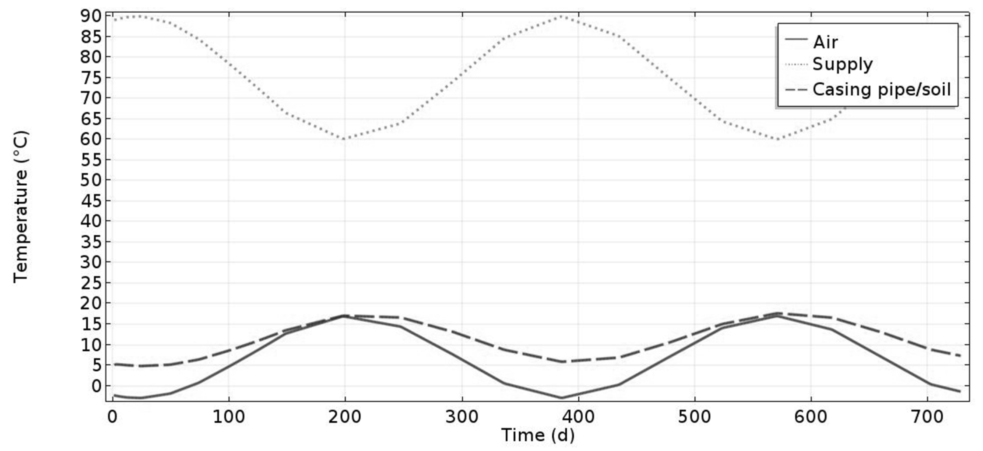
5.1. Soil Temperature at Casing Pipe

The numerical calculations of the temperature decline in the DH pipe involve the thermal properties of the pipe and the water volume, and also the soil temperature. The soil temperature (i.e., casing pipe temperature) has been assessed through numerical transient calculations using COMSOL Multiphysics, which was assessed to be handier than Matlab for visual analyse. The soil layer above the DH pipe consists of 0.8 m of sand with a thermal conductivity of 1.5 W/mK, a density of 2500 m3/kg, and a heat capacity of 840 J/kgK. The soil temperature is calculated with seasonal variations using Equations (6) and (7) [14,15].
T e ( t ) = T aa + T A sin ( 2 π ( t t d ) t p )
T f ( t ) = T a f T A f sin ( 2 π ( t t d ) t p )
Here, T e ( t ) is the exterior ambient temperature, T aa is the annual average air temperature at the soil surface, T A is the seasonal amplitude of the ambient temperature,   t d is the time delay (113.5 days for the Swedish climate), t p is the total duration of the period (one year), and t is time ( t = 1 represents the first of January). The supply temperature in the DH pipe, T f ( t ) , is calculated in a similar way, using the annual average supply temperature, T a f , and the seasonal amplitude of the supply temperature, T A f . From the numerical calculations in Figure 10 it can be seen that the casing pipe temperature varies between 6 and 17 °C (1–14 °C without the DH pipe as a heat source). The casing pipe temperature in April, the time of these cooling tests, is approximately 12 °C.
As seen from Figure 10, both the supply and air temperatures influence the soil temperature, T s , at the casing pipe. However, one can roughly estimate the soil temperature using the simpler Equations (8)–(10) without considering the seasonal air temperature variations [16,17].
T s = R i T e + R s T f R i + R s
Here, R i (K/W) is the thermal resistance of the pipe insulation, T e is the average air temperature at the soil surface (during the actual month), R s (K/W) is the thermal resistance of the soil, and T f is the fluid temperature (monthly average).
R i = 1 2 π λ i ln D P U R d o
R s = 1 2 π λ s ln 4 Z c D c
Here, λ i (W/mK) is the estimated thermal conductivity of the PUR insulation, D P U R (m) is the diameter of the PUR insulation, d o (m) is the outer diameter of the service supply pipe, λ s (W/mK) is the thermal conductivity of the soil, Z c is a corrected value of the distance from the soil surface to the pipe centre Z (m) with respect to surface transition resistance, R o , where Z c = Z + R o λ s and R o can usually be valued at 0.0685 (m2 K/W) [16], and D c is the radius of the casing pipe.
Calculation using the simpler Equation (8) results in a soil temperature of 13.2 °C, which can be compared with the numerical calculation that resulted in a soil temperature of approximately 12 °C for the same month.

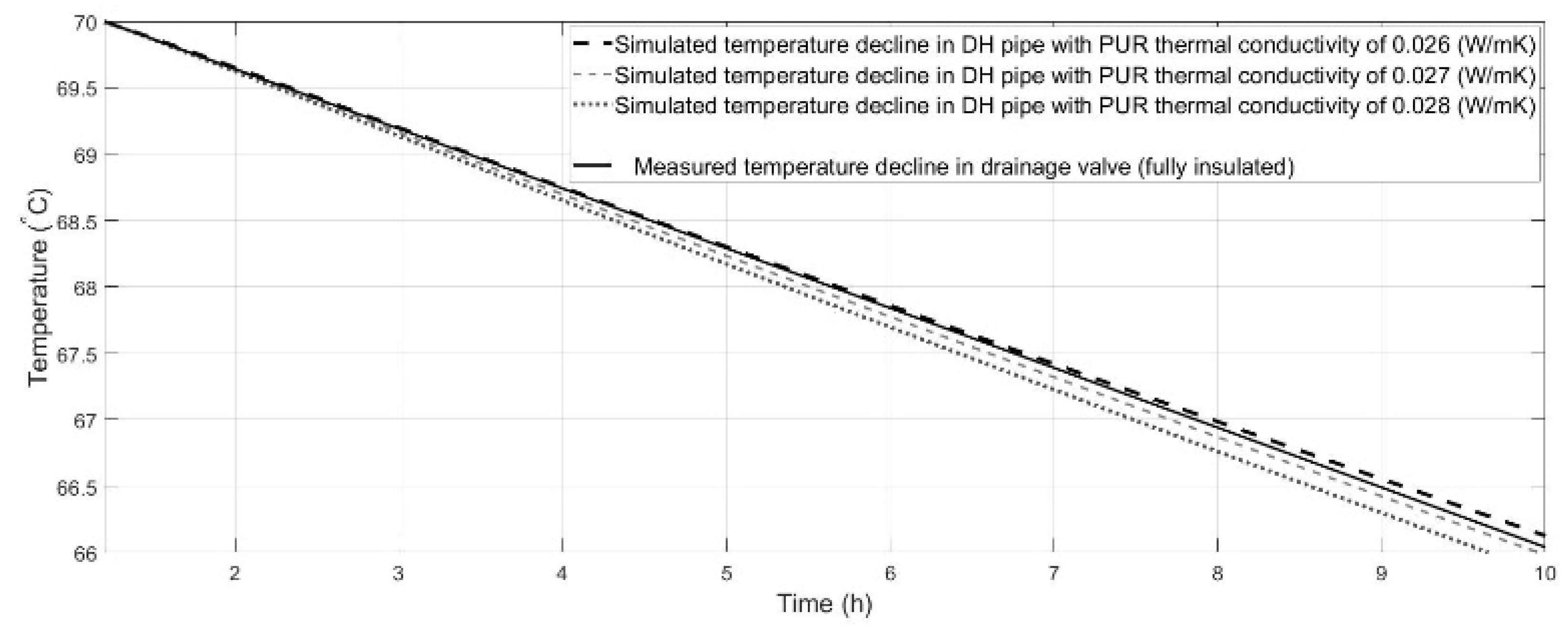
5.2. Resulting Thermal Conductivity in the DH Pipe

In Section 4, the drainage valve was shown to represent the actual temperature decline in the DH pipe with high accuracy. The mean temperature decline is calculated from the drainage valve measurements during the three shutdowns in the field test. The mean decline is then compared to numerical simulations of the temperature decline in the DH pipe according to the model presented by Lidén et al. [10]. Figure 11 shows that with a thermal conductivity of 0.026–0.027 W/mK for the PUR in the DH pipe, a good match is found between the simulated and measured temperature decline, i.e., the actual status of the evaluated two-year-old operating DH pipe. This can be compared to newly produced pipes, which, according to the manufacturer, should have a thermal conductivity of 0.026 W/mK [18], resulting in a slope of 0.44 °C/h in the present soil. The soil temperature at the casing pipe is calculated to be 12 °C. A sensitivity analysis of the casing pipe temperature indicates that misjudgement of soil temperature would lead to an error in the thermal conductivity of the PUR of approximately 1.4% per degree Celsius, i.e., even if the simpler Equation (9) is used (see Section 5.1), a highly accurate assessment can still be conducted. Hence, calculation results in a soil temperature of 13.2 °C and thereby approximately the same conductivity.
The slope of 0.44 °C/h for newly buried pipes can also be compared with the results in Table 4, where the slopes were 0.44–0.46 °C/h for the fully insulated drainage valve, a difference of less than 5%.

6. Suggested Method for Assessing the Thermal Performance of PUR Insulation

The cooling method, a non-destructive testing method for estimating the thermal status of a DH pipe in operation, can be conducted given the following prerequisites:
  • An accessible manhole with a shutdown valve for turning the flow off and on.
  • At least one measurable drainage valve accessible through a manhole in the assessed part of the network. The drainage valve should be insulated with at least hat insulation (see Section 2). Installing the manhole set-up and starting recording with the temperature logger should be performed at least 2 h before the shutdown.
  • The DH network under assessment should be shut down for at least 2 h for pipe dimensions up to DN200 and for at least 8 h for pipe dimensions up to DN500. The required shutdown time can be adequately estimated by dividing the nominal diameter (DN) by 60, i.e., DN500/60 = 8.3 h.
  • The cooling method is assessed to have a margin of error of less than 5% if estimates of the following parameters are known: thermal conductivity of the soil (rough estimate), supply temperature data from nearby customers, pipe depth from soil surface, and seasonal air temperature variations on location.

7. Conclusions

A general diagnostic protocol for the thermal assessment of a DH pipe in operation has been presented. A new improved measurement set-up for a field test of the cooling method has been analysed. The results further support the previously highlighted drainage valve as the best and most accessible point for measuring the thermal status of a buried DH network. Both the drainage and shutdown valves were analysed numerically using new FDM models and the results were compared with field test measurements. Satisfactory results could be obtained from the drainage valve in terms of the accuracy of capturing the temperature decline in the DH pipe. However, the shutdown valve could not yield sufficiently accurate results, despite the present improved set-up, and has to be dismissed as a measurement point. Finally, the cooling method using the drainage valve as a measurement point allowed the thermal conductivity of the buried DH pipe in operation to be assessed with an accuracy of >95%.

Author Contributions

Conceptualization, P.L. and B.A.-Z.; methodology, P.L.; software, P.L.; validation, P.L., B.A.-Z. and C.-E.H.; formal analysis, P.L.; investigation, P.L.; data curation, P.L.; writing—original draft preparation, P.L.; writing—review and editing, B.A.-Z. and C.-E.H.; visualization, P.L.; supervision, B.A.-Z. and C.-E.H.; project administration, P.L. All authors have read and agreed to the published version of the manuscript.

Funding

This research received no external funding.

Conflicts of Interest

The authors declare no conflict of interest.

References

  1. Fredriksen, S.; Werner, S. District Heating and Cooling, 1st ed.; Studentliteratur AB: Lund, Sweden, 2013. [Google Scholar]
  2. Berge, A.; Adl-Zarrabi, B.; Hagentoft, C.-E. Assessing the Thermal Performance of District Heating Twin Pipes with Vacuum Insulation Panels. Energy Procedia 2015, 78, 382–387. [Google Scholar] [CrossRef] [Green Version]
  3. Zwierzchowski, R.; Niemyjski, O. Simulation of Heat Losses of a Distribution Network with Different Technical Structure and under Different Operating Conditions for a District Heating and Cooling System. IOP Conf. Ser. Mater. Sci. Eng. 2019, 603, 032091. [Google Scholar] [CrossRef]
  4. Danielewicz, J.; Śniechowska, B.; Sayegh, M.A.; Fidorów, N.; Jouhara, H. Three-dimensional numerical model of heat losses from district heating network pre-insulated pipes buried in the ground. Energy 2016, 108, 172–184. [Google Scholar] [CrossRef] [Green Version]
  5. Chicherin, S.; Mašatin, V.; Siirde, A.; Volkova, A. Method for Assessing Heat Loss in A District Heating Network with A Focus on the State of Insulation and Actual Demand for Useful Energy. Energies 2020, 13, 4505. [Google Scholar] [CrossRef]
  6. Wang, H.; Meng, H.; Zhu, T. New model for onsite heat loss state estimation of general district heating network with hourly measurements. Energy Convers. Manag. 2018, 157, 71–85. [Google Scholar] [CrossRef]
  7. Lidén, H.P.; Adl-Zarrabi, B. Non Destructive Methods of District Heating Pipes. In Proceedings of the 12th ECNDT, Gothenburg, Sweden, 10–19 June 2018. [Google Scholar]
  8. Lidén, H.P.; Adl-Zarrabi, B. Development of a Non-destructive Testing Method for Assessing Thermal Status of District Heating Pipes. J. Nondestruct. Eval. 2020, 39, 22. [Google Scholar] [CrossRef] [Green Version]
  9. Lidén, P.; Adl-Zarrabi, B. Non-Destructive Methods for Assessment of District Heating Pipes: A Pre Study for Selection of Proper Method. In Proceedings of the 15th International Symposium on District Heating and Cooling, Seoul, Korea, 4–7 September 2016. [Google Scholar]
  10. Lidén, H.P.; Adl-Zarrabi, B.; Hagentoft, C.E. Diagnostic Protocol for Thermal Performance of District Heating Pipes in Operation. Part 1: Estimation of Supply Pipe Temperature by Measuring Temperature at Valves after Shutdown. Energies 2021, 14, 5192. [Google Scholar] [CrossRef]
  11. Fjellborg, F. Data Received from Borås Energy; Borås Energy: Borås, Sweden, 2021. [Google Scholar]
  12. Miller, D. Advances in Heat Transfer; Irvine, T.F., Jr., Hartnett, J.P., Eds.; Academic Press: New York, NY, USA, 1964; Volume 1, p. 459. [Google Scholar] [CrossRef]
  13. MathWorks. Available online: https://www.mathworks.com/help/matlab/ref/ode15s.html (accessed on 16 August 2021).
  14. Hagentoft, C.E. Introduction to Building Physics; Ligthning Source: Lund, Sweden, 2001. [Google Scholar]
  15. Swedish Meteorological and Hydrological Institute. Available online: www.smhi.com (accessed on 16 August 2021).
  16. SS-EN13941. Design and Installation of Preinsulated Bonded Pipe Systems for District Heating; Swedish Standards Institute: Stockholm, Sweden, 2009. [Google Scholar]
  17. Claesson, J.D.A. Heat Extraction from the Ground by Horizontal Pipes—A Mathematical Analysis; Sweden, L., Ed.; Department of Mathematical Physics, Swedish Counsil for Building Research: Stockholm, Sweden, 1983; Volume D1. [Google Scholar]
  18. Powerpipe. Product Catalog; 2018; Available online: www.Powerpipe.se (accessed on 4 February 2021).
Figure 1. Pipe network and measurement location. (C) measurement point for analyses (i.e., valves). (D) supply flow shutdown point. Ordinary flow direction is (AE). During shutdown at valve point (D), the flow between (B,D) (dashed line) stops and new flow towards (E) is only via (F). Supply water is shown in black and return water in grey.
Energies 14 05302 g001
Figure 2. (a) Measurement set-up in manhole C showing the thermocouples installed in the manhole prior to insulation; (b) manhole C fully insulated after installation of thermocouples, except for the 250-mm free space (air); (c) thermocouple placement in manhole C (not to scale); and (d) thermocouple placement in manhole D.
Energies 14 05302 g002
Figure 3. Non-dimensional parameter, u, at the sensor for length L of the rod; the dimensional length a t L is used.
Energies 14 05302 g003
Figure 4. Slope function 1 β d T v d t versus the dimensionless time for the shutdown valve.
Energies 14 05302 g004
Figure 5. Measurement results from thermocouples, with a focus on the shutdown valve.
Energies 14 05302 g005
Figure 6. The figure shows the water inside the drainage extension pipe, flowing upwards in the core and downwards at the periphery. Note that there is no insulation on the top part of the valve in this figure.
Energies 14 05302 g006
Figure 7. Temperature sensor response after a step change in supply temperature at time zero. The initial temperature in the drainage valve pipe is 90 °C at t = −10 h; at time zero, the supply temperature drops to 70 °C.
Energies 14 05302 g007
Figure 8. The modelled sensor temperature (solid line) as a function of the time after the change in the supply pipe temperature. The dashed line shows the supply pipe temperature, with a temperature drop starting at time zero (the first hour is slow due to the thermal response time). The initial temperature in the drainage valve pipe is 90 °C at t = −10 h. At time zero the supply temperature starts dropping from 90 °C at 1 °C /h.
Energies 14 05302 g008
Figure 9. Measurement results for thermocouples with a focus on the drainage valves; the shutdown valve is included for comparison.
Energies 14 05302 g009
Figure 10. Seasonal variations in the casing pipe/soil temperature over two years; numerical calculations conducted in COMSOL Multiphysics.
Energies 14 05302 g010
Figure 11. Measured average temperature decline in the drainage valve after the thermal response time during the three shutdowns versus simulated temperature decline in DH pipe with PUR thermal conductivity of 0.026–0.028 W/mK.
Energies 14 05302 g011
Table 1. Calculated matching factors for the two valve types with their standard deviations; data for hat insulation are from previous tests [10].
Shutdown Valve, Hat InsulatedShutdown Valve, Fully Insulated
Matching factor0.710.53
Standard deviation0.280.05
Table 2. Thermal response time and slope of temperature decline during cooling for the shutdown valve; data for hat insulation are from previous tests [10].
Shutdown Valve, Hat InsulatedThermal Response Time (min)Temperature Decline (°C/h)Shutdown Valve, Fully InsulatedThermal Response Time (min)Temperature Decline (°C/h)
First shutdown5100.37First shutdown--
Second shutdown3370.44Second shutdown3520.17
Third shutdown2700.33Third shutdown2630.29
Table 3. Calculated matching factors for the drainage valves, with their standard deviations.
Drainage Valve, UninsulatedDrainage Valve, Hat InsulatedDrainage Valve, Fully Insulated
Matching factor0.280.120.05
Standard deviation0.040.060.03
Table 4. Thermal response time and slope of temperature decline during cooling for the drainage valve; data for hat insulation from previous tests [10].
Drainage Valve,
Hat Insulated
Thermal Response Time (min)Temperature Decline (°C/h)Drainage Valve, Fully InsulatedThermal Response Time (min)Temperature Decline (°C/h)
First shutdown700.43First shutdown410.45
Second shutdown430.45Second shutdown450.44
Third shutdown330.44Third shutdown540.46
Publisher’s Note: MDPI stays neutral with regard to jurisdictional claims in published maps and institutional affiliations.

