Article

Economic Dispatch of CHP Units through District Heating Network’s Demand-Side Management

1
Narva Soojusvõrk AS, Oru 2, 20203 Narva, Estonia
2
Department of Energy Technology, Tallinn University of Technology, 19086 Tallinn, Estonia
*
Author to whom correspondence should be addressed.
Energies 2021, 14(15), 4553; https://doi.org/10.3390/en14154553
Submission received: 22 June 2021 / Revised: 21 July 2021 / Accepted: 26 July 2021 / Published: 28 July 2021
(This article belongs to the Special Issue Recent Advances in District Heating)

Abstract

:
Optimisation of heat and electrical load distribution, where the objective function is the maximum efficiency of the CHP unit for a given load range, can be done considering the limitations of electrical power and the heat load. Simulating a real CHP unit with a district heating network shows that demand-side management can improve the overall economic efficiency of the CHP plant and increase the unit’s operating range in the electricity spot market. Economic dispatch makes it possible to determine a reasonable additional increase in the electric power of the CHP unit, and to optimise the supply temperature and mass flow of the district heating network. The results obtained and the analysis performed indicate that the proposed methodology provides logical results and can be used to calculate the efficiency indicators of the cogeneration of electrical and thermal energy. The problem of optimising the operating mode of the CHP unit was solved, which allows us to determine the optimal additional increase in the unit’s electrical load at a given heat load of consumers, which on average increases the CHP unit’s efficiency up to an additional 1.5%.

1. Introduction

In today’s European district heating networks, about three-quarters of the total heat supply is provided by CHP units. Since the beginning of 2013, the Estonian electricity market has been fully open to all electricity consumers and is run by Nord Pool. Electricity generated simultaneously with heat can be sold on the spot markets. Due to the increase in the variance of the price of electricity, it is important for the profitability of the CHP unit to produce electricity when the price is high. Of course, the demand for thermal energy will never be fully synchronised with the demand for electricity [1].
The traditional goals of economic dispatch of CHP units are minimising operation cost and maximising profits [2]. Optimisation of heat and electrical load distribution, where the objective function is the maximum efficiency of the CHP unit for a given load range, can be done considering the fact that electrical power is limited by the heat load. The main problem of CHPs is that their operation is highly dependent on the heat load, which makes them rather inflexible or reduces the overall efficiency during periods of insufficient heat load (condensing turbine [3]).
The combined heat and power economic dispatch problem is formulated as an optimization problem [4]. A practical economic dispatch problem should include minimum and maximum limits for power and heat generation of CHP unit, which makes searching for the optimal dispatching a challenging problem [5]. The optimal economic dispatch for various types of CHP plants was analysed in [6]. In [7], the flexibility of CHP and thermal energy storage was explored using a two-stage optimal dispatch, considering the day-ahead heat market and real-time wind power balancing. There are also some studies focusing on solving the district heating operation problem together with the optimal dispatch for the electric power system [8,9,10]. Electricity and heat networks were investigated as a whole by combined analysis in [11].
In recent studies, global optimisation techniques, such as genetic algorithms [12], the harmony search algorithm [13], and particle swarm optimisation [14], have been used for the optimal tuning of CHP economic dispatch-based restructure schemes.
In this paper, maximum overall efficiency and heat and power output for each heat demand are obtained using advanced calculus methods that involve the Lagrangian function [15], where the problem is to determine the power and heat produced by the CHP unit so that the system’s overall production efficiency is maximised while the demand for power and heat, as well as other constraints, are met.
The importance of demand-side management for heat production efficiency was discussed using the example of a CHP unit that is flexible due to the coupling of heat and power energy vectors and provides real-time demand-side management [16], to external market signals, thus boosting their overall business case with respect to classic load following operation [17]. Following the preliminary work done in [18], this paper proposes a case-based system-level modelling approach that provides an innovative and integrated analysis of optimal and dynamic (as in real-time demand-based) control of CHP plants under uncertain market prices.
According to the fourth-generation district heating concept, decentralised intelligent metering is an important aspect of sustainable district heating [19]. Wireless collection of heat meter readings makes it possible to gather hourly data on each consumer. Decentralised intelligent metering allows one to collect additional information on consumer behaviour, providing DH companies with numerous advantages, such as the ability to effectively manage the grid, increase production efficiency, optimise thermal energy storage, and quickly identify faults at substations [20]. The technology of decentralised smart metering is well-developed and successfully used in district heating systems. More than 70% of the district heating companies in Estonia have remote metering [21]. The proportion of decentralised smart metering in Narva’s district heating system is 100% [22]. Collecting detailed heat demand data using hourly smart metering can improve the efficiency of CHP heat and electricity production by applying the economic dispatch approach to demand-side management. Without demand-side management and smart metering, heat loads were determined based on the outdoor temperature, statistical data, and temperature measurements of the heat carrier in the district heating network [23,24].
Some researchers have proposed an analysis of the potential of a return temperature differential regulation strategy for substation control to reduce the thermal peak in the DH system [25]. Changes in the schedules of the heating systems installed in the buildings used for virtual storage application were studied in [26]. The energy consumption planning problem was formulated both for individual substations and for the district heating operator in [27]. In [28], an electricity and heat coordinated retail market framework was proposed to achieve coordinated shedding of electrical and heat loads, and to manage the district’s energy generation and consumption through transactive control methods. In [29], the main focus was on ensuring that data that were automatically collected in substations were suitable for modelling purposes, for automatically detecting fouled heat exchangers, forecasting the thermal request evolution of the building, as well as determining the proper use of demand-side management based on network dynamics. Another approach to achieving peak shaving is using demand-side management, also called demand response or virtual storage [30]. The estimation of a thermal request is performed using a black box approach consisting of a linear programming model that provides the main characteristics of the curve for a given set of inputs using experimental data [31]. The best peak shaving should be evaluated at the plant level. Plant load is not the same as the sum of thermal requests in buildings, because it is influenced by the thermal transient processes in the network additionally [29]. Several articles demonstrate an interest in achieving higher performances and flexibility in [32].
The benefits of heat consumption forecasts include the identification of demand response actions and peak power demand [24]. Demand-side management is the cost-effective management of complex DH systems that must include the rationalisation of the operations of all components involved in heat production and distribution [25]. Demand-side management uses demand process data related to production status, heat distribution, and weather forecasts to manage production and heat distribution, and tools that allow for the dynamic calculation of control parameters that help achieve maximum efficiency while ensuring adequate heat supply [26].
Demand-side management allows multivariate calculations to determine the expected CHP indicators for the forecast period based on the outdoor temperature and the range of possible deviation. A special role is currently played by short-term forecasting for one day for the participation of power units in the formation of the electric schedule based on the results of open market trading. Taking into account the obtained heat load forecast, it is possible to choose the optimal hourly loads and submit the most favourable price offers.
Thus, there is a need for justification and an adequate mathematical relationship describing the process of changing the heat load depending on several parameters that have a direct impact on the change. The results of the study will make it possible to create the most effective and cost-efficient technical solutions to optimise the operating modes of thermal power units.
Demand-side data were used to identify and validate the heat demand model. This model can be used to replace the simplified average heat load approach to predict the potential electrical load to create an offer for the wholesale electricity market.
The optimisation algorithm performs the following actions:
-
Analysis of entered data to ensure that it adheres to existing restrictions;
-
Selection of power modes from the database that satisfy the given loads and consider the imposed external constraints;
-
Optimization of the distribution of heat and electrical loads of each mode as a function of many variables with linear constraints, such as inequalities and balance equations for the electrical and heat loads of the CHP unit.
Thus, the model uses regression analysis of the empirical dependence of the thermal energy demand on the outdoor air temperature to predict the thermal energy demand with a high degree of accuracy of approximation of the actual demand measurement results. Demand-side management with consumer input also minimises the risk of data errors, while forecasting can reduce potential losses from production efficiency, calculate future consumption demand for each user, and determine total demand.
The study develops in four sections. After introducing and highlighting aspects of the literature in Section 1, Section 2 of the article provides the materials and methods, an overview of the methodology for economic dispatch modelling through demand-side management. Section 3 presents the discussion and Section 4 presents the study results of the model validation using the example of Narva’s district heating network and the fossil-fuelled Balti Power Plant CHP unit that provides heat to the DH network. The conclusions are presented in Section 5.

2. Materials and Methods

2.1. Problem Formulation

One of the problems in heat sales management is the inability to estimate the future supply for each customer [33]. Since thermal energy cannot be supplied in a volume that exceeds the real demand for it, the surplus must be minimised at the sales planning stage. This can be done by using an automatic system for calculating demand, which includes individual heat meters and a tool for predicting heat demand [29]. With the help of forecasting, an objective assessment of the current state of control over the sale of heat becomes possible [26]. The main task of the forecasting tool is to calculate individual demand for each customer based on their recorded demand data from the database [34].
The proposed model based on thermal energy demand-side data is dynamic and uses a database of remotely transmitted hourly heat demand data. This makes it possible to use a model instead of statistical data during planning. In this case, obtained data will be based on regression dependences on the values of the current regime parameters of demand, depending on the outside air temperature. By summing the demand data of all customers and taking into account the losses determined via the balance method as the difference between production and demand for thermal energy for the predicted outdoor temperature, we can predict the heat demand for each hour.
The main advantage of this model when solving the forecasting problem compared to models based on information for the past period is that the resulting model can take into account previously unknown information about district heating networks. This information includes changes in heating networks, their reconstruction, the transition to new conditions of demand, and the emergence of new installations among consumers during the predicted period. Taking account of these changes leads to a decrease in the forecast error. Demand-side management data are measured at thermal substations with an automatic download of historical data for each substation. Based on these data, we can obtain a consumption profile for each facility, depending on the outdoor temperature.
Solving the problem of predicting the heat demand of objects will help to determine the amount of heat that will be consumed in the coming periods of time. Each object has a static characteristic that describes its thermal load. This characteristic is static in the sense that it cannot be changed quickly. Therefore, it is very informative for various types of heat demand analysis.
Mathematically, this characteristic is described by the functional dependence: Q = f (Toutdoor), where Q is the amount of thermal energy consumed (MWh) and Toutdoor is the outdoor air temperature (°C), allowing us to find a straight line as close as possible to the data points from the heat metering unit. With a high degree of approximation accuracy, it is possible to use a linear function to solve the forecasting problem. To construct and analyse this dependence, one should use the instantaneous demand data from the remote reading system of heat meters.

2.2. Demand-Side Management

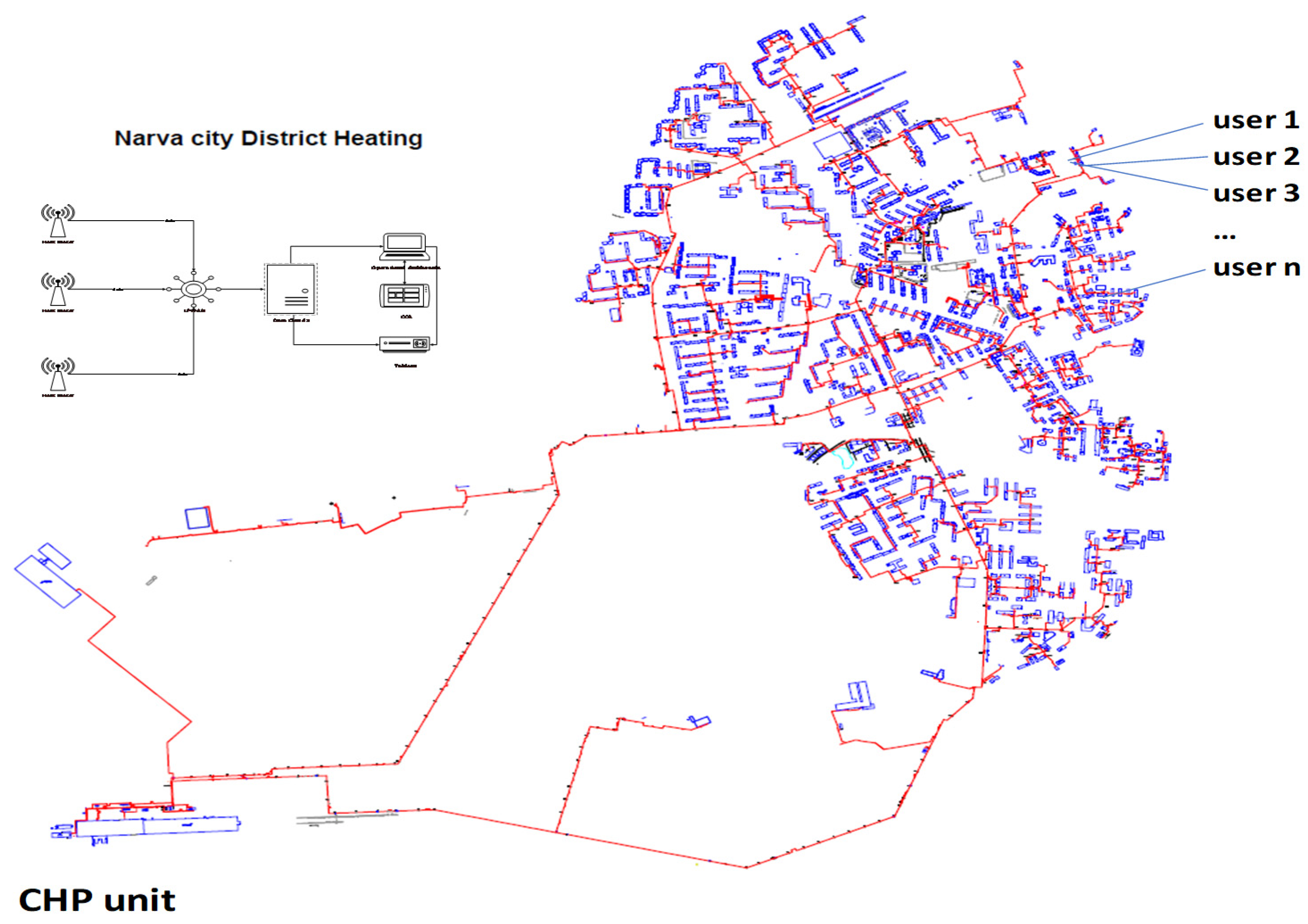
The demand-side data for each substation was measured and collected by smart meters every hour for the entire distribution network (730 buildings), which is shown in Figure 1. An automatic system evaluates data outside a meaningful range and fills them in via interpolation. The automatic evaluation of the curve characteristics of all consumers is used to simplify the hourly evolution of the next day’s thermal request to easily predict the thermal request.
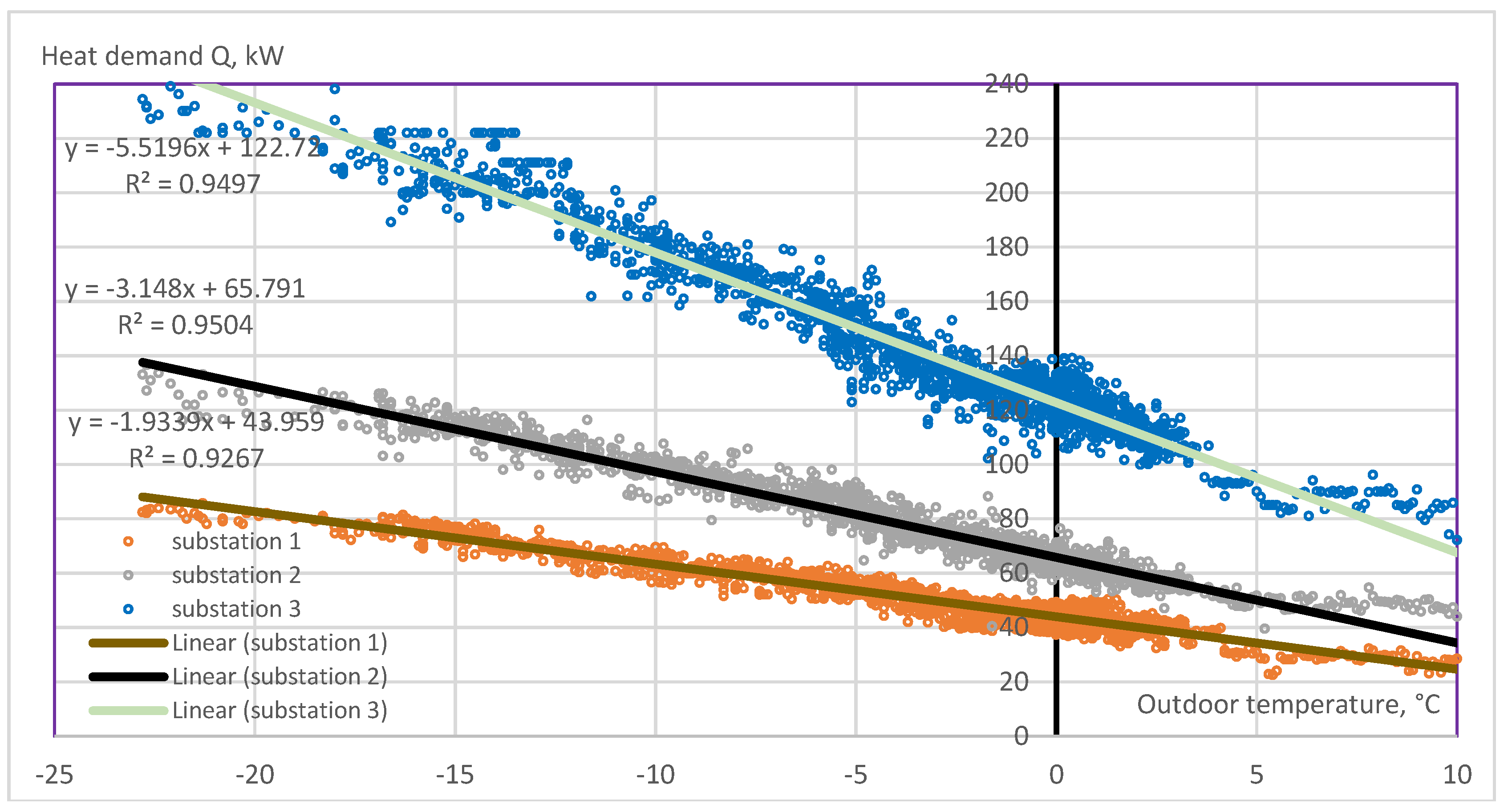
Outdoor temperature and heat demand are measured every hour for each substation. Examples of this dependence for three selected substations using data collected during the 2020/2021 heating season (October–April) are shown in Figure 2.
As can be seen from the above diagram, this dependence is nearly linear. An important area of application of this model is the solution of forecasting problems. To predict the generation and consumption of thermal energy and heat losses for a short-term period of 24 h, the first task is to understand the variability of each consumer. To do this, we must calculate the demand-side of hourly demand for each consumer via a histogram, an example of which is shown in Figure 2. The y-axis in the graph represents the various hourly demand points and the x-axis represents the outdoor temperature. Based on the consumption data, we have linear characteristics for each object of thermal energy demand. The second task is to understand the influence of the outdoor air temperature on the heat demand of each consumer.
The final step of the algorithm for the next day’s daily profiles is to extract the daily demand hours that occur regardless of the outdoor air temperature. To do this, we use the periodic autoregressive algorithm for time series data from a fragment of an hourly demand time series for all consumers over a period of several days. We are only given the total hourly demand, but the purpose of the algorithm is to determine, for each hour, which load does not depend on temperature and which additional load is temperature related.
The demand-side management approach considered in this paper has x users and y heat sources as the research objects, and the set of all users is represented as X = (1 … x). The number of heat sources Y is denoted by numbers 1 … y. The relationship between the heat produced by heat source y and its users is represented as f(y) = (y1yx), where f(yx) indicates that the heat is supplied to user x over time T. If the heat loss in the system is not taken into account, then the heat supplied to user x by the heat source is equal to the heat dissipated by user x (see Equation (1)).
H u s e r x = c × ( t 1 x t 2 x ) × m x × T ;   x = 1 n ( H u s e r ) = H d e m a n d
where t1x and t2x are the supply and return temperatures of user x (°C). mx is the flow rate of user x (kg/h); c is the water mass/specific heat of water mass (4.19 kJ/(kg⋅°C))
The heat supplied by heat source y is
Q s y = c × ( t 1 y t 2 y ) × m y × T
where t1y and t2y are the water supply and return temperatures of heat source y (°C). my is the circulating flow rate of heat source y (kg/h).
The demand-side data collection system allows us to identify the optimal set of user heating system turn-on times, which is necessary to assess the expected thermal profile of each building. Temperature sensors collect temperature data at the inlet and outlet of heat exchangers, and mass flow meters measure the current mass flow rate. These data can be used to estimate the change in heat demand for a monitored consumer at different outdoor air temperatures. This way, it is possible to estimate the consumer’s heat load profile for different outdoor air temperature levels.
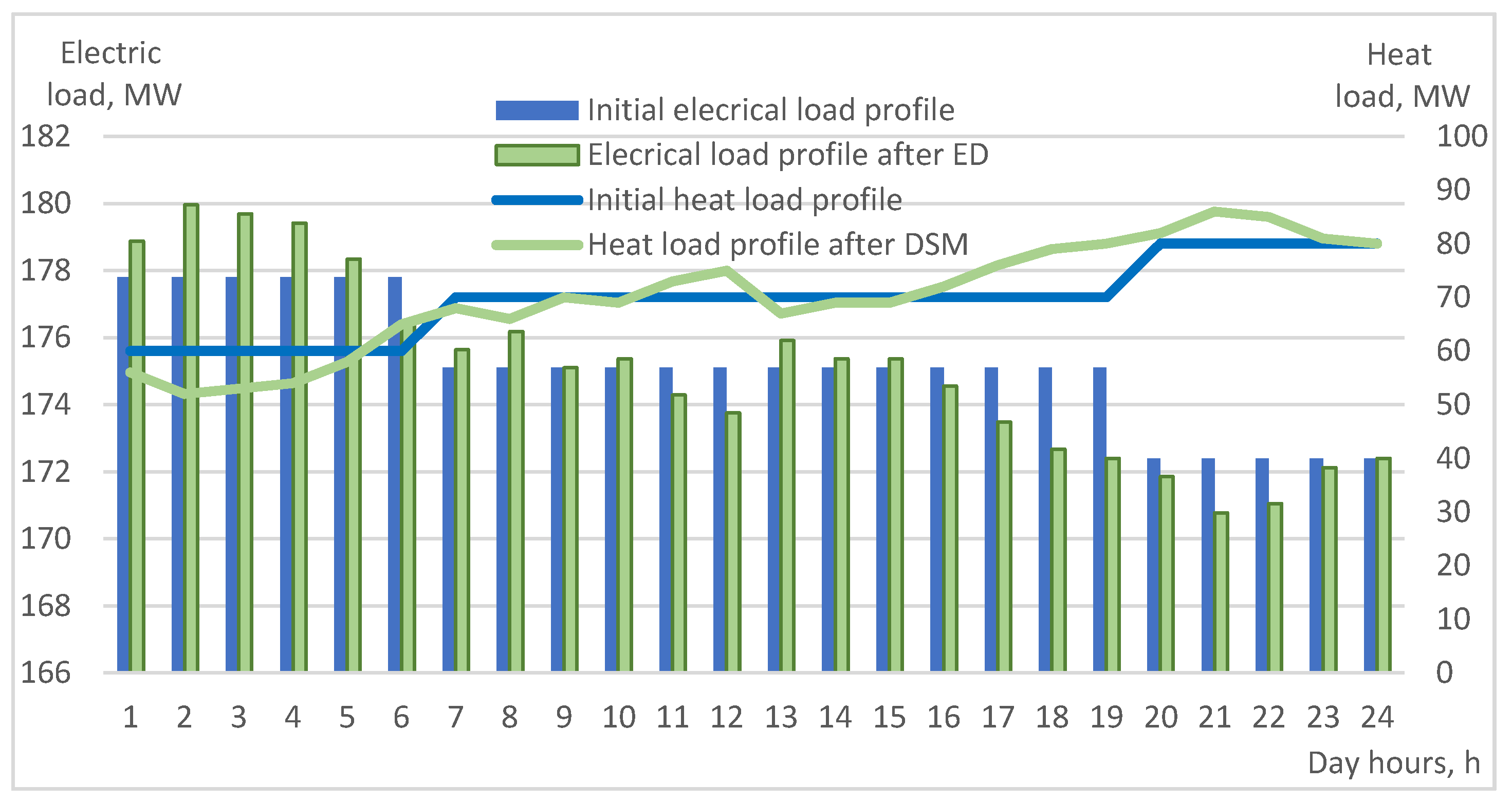
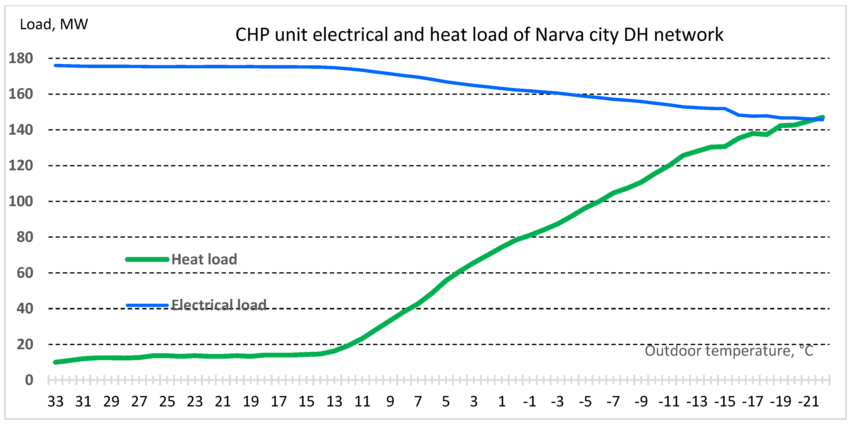
It is always necessary to satisfy the heat demand, even if the electrical load and the heat load of the CHP unit are interrelated. A typical profile of the average load for a CHP unit before the application of the model and after optimisation with more accurate consumption data is shown in Figure 3.
Based on the assessment of all possible combinations of electrical and thermal loads, it is possible to find the general optimum for each mode of operation of the unit. It is necessary to minimize the consumption of primary energy of the CHP or its overall efficiency at the given electrical and thermal loads of the unit for more accurate planning. Economic Dispatch is applied at each settlement hour by optimizing the distribution of heat and electrical loads based on heat demand-side data.

2.3. Combined Heat and Power Generation

The model used in this article was based on the CHP plant and district heating network in the city of Narva (in north-eastern Estonia). The district heating company supplies heat to about 60,000 residents. Narva’s district heating network is 78 km long and connected to 730 buildings. Heat is generated at the Balti Power Plant (CHP unit), which consists of two circulating fluidized bed boilers, including one reheat and steam turbine, which is a three-casing reheat condensing impulse reheat turbine with uncontrolled extraction for seven stages of feedwater heating. The fuel used in the Balti Power plant is local fossil fuel oil shale mixed with wood chips [35]. The DH circulating water is heated in a district heater using steam from the crossover pipes between the intermediate-pressure and low-pressure parts of the turbine. Extra steam from the hot reheat steam line is supplied to the peak load and the auxiliary steam is supplied to an external auxiliary steam header. The maximum DH load of the facility is 160 MW and the maximum water outlet temperature is 130 °C. The DH inlet water temperature ranges from 40 °C to 60 °C. The annual heat demand in Narva is about 450 GWh. The unit’s annual electricity production is approximately 1300 GWh. The main inputs for these analyses are electricity and heat production and process efficiency as per the data available.
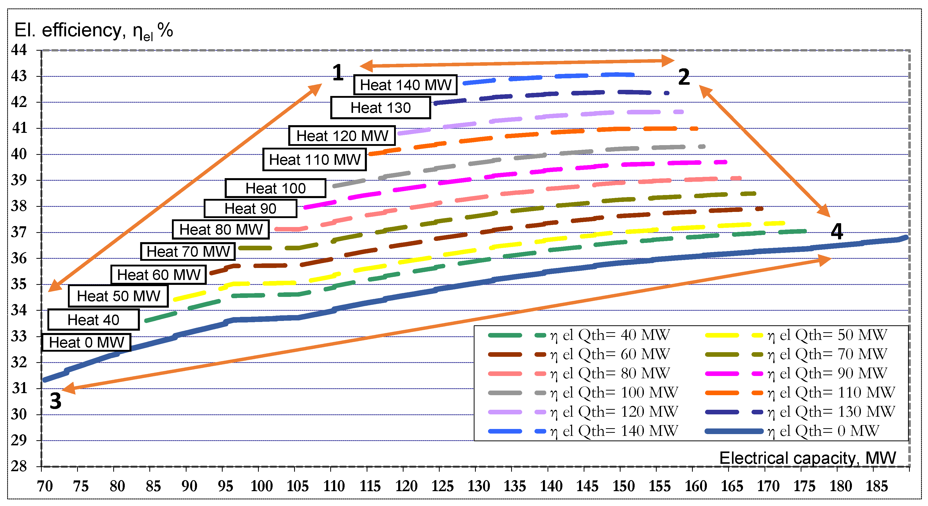
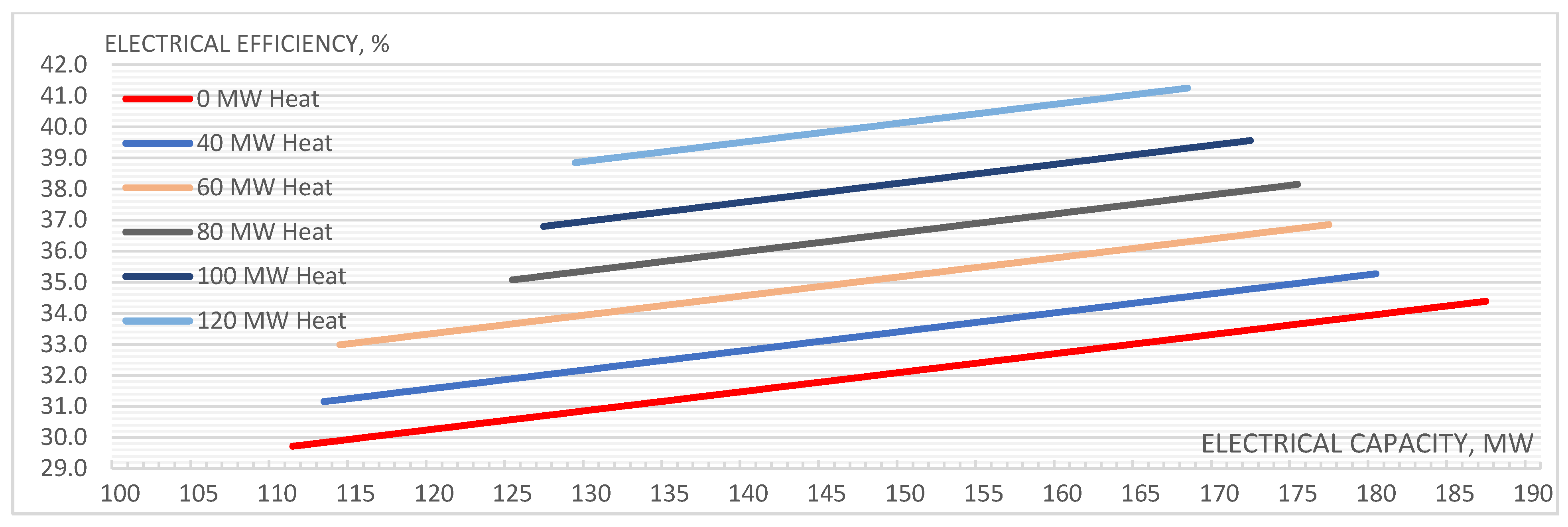
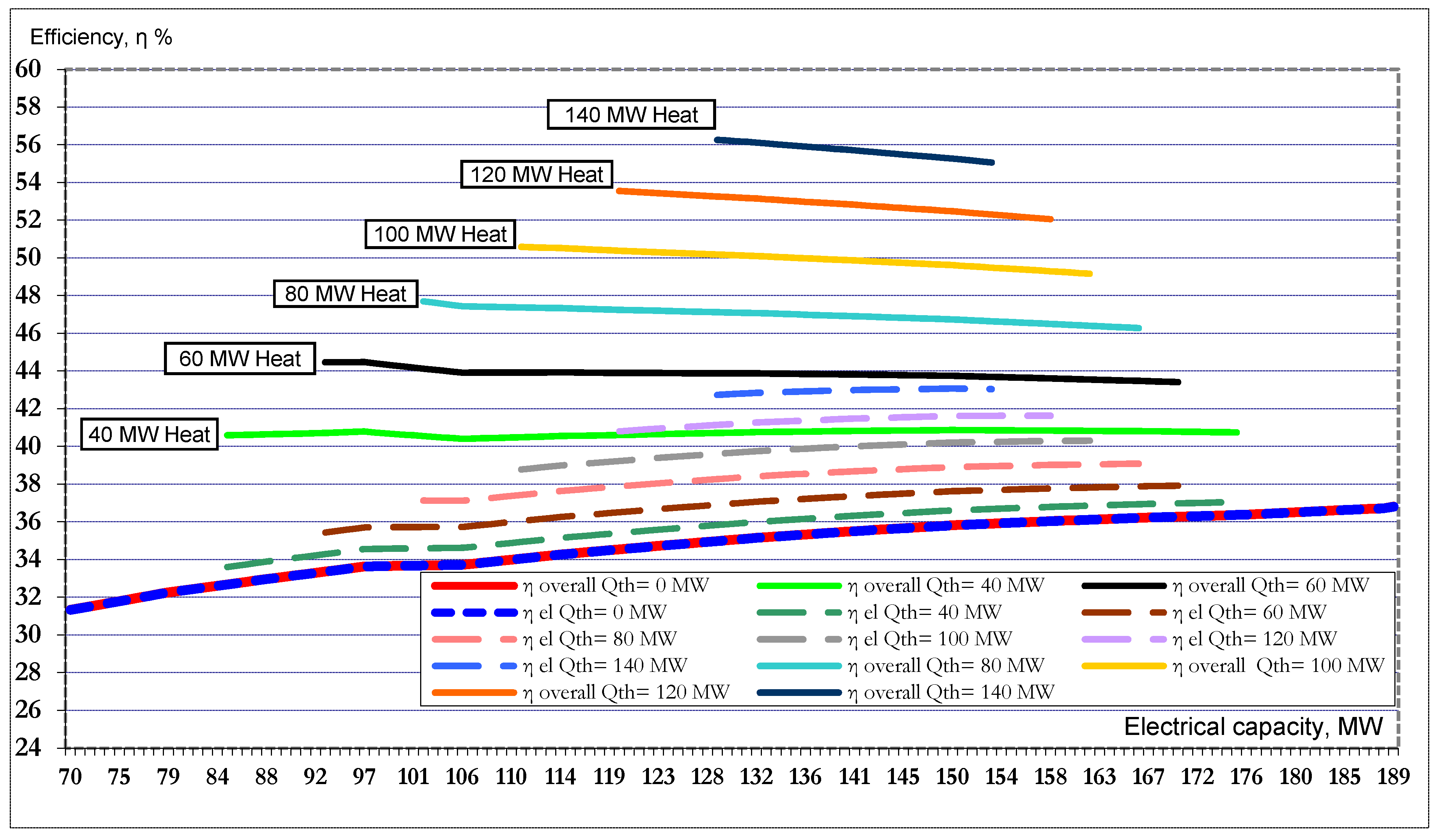
The efficiency characteristic of a CHP unit depends not only on the electrical load, but also on the amount of heat supplied. The electrical efficiency dependence on the electrical load of the CHP unit for different heat loads is shown in Figure 4.
Points 1, 2, 3, and 4 have been added to Figure 4 for more clear presentation of CHP operation modes:
1–2—CHP operating at 100% heat load;
3–4—CHP operating without heat extraction;
3–1—limitation on the minimum electrical load to ensure the parameters of heat supply;
2–4—limitation on the maximum electrical load to ensure the amount of heat supply.
It can be seen that electrical efficiency is increased when the heat load becomes larger. When the heat load is maximum, the electrical load is lower (150 MWnet). The maximum electrical load (190 MWnet) is possible when there is no heat load, but in this case, electrical efficiency is the lowest.
The mathematical optimisation model of a CHP establishes the dependence of primary energy consumption Bi on the value of heat (Hi) and electrical (Ei) loads when operating according to an electrical schedule: Bi = f (Ei). When operating on a heating schedule, the electric power depends on the heat load, so the objective function takes the form of Bi = f (Ei, Hi). Short-term optimisation has a horizon of one day, discreteness Δi = 1 (one hour), and timestamps i.
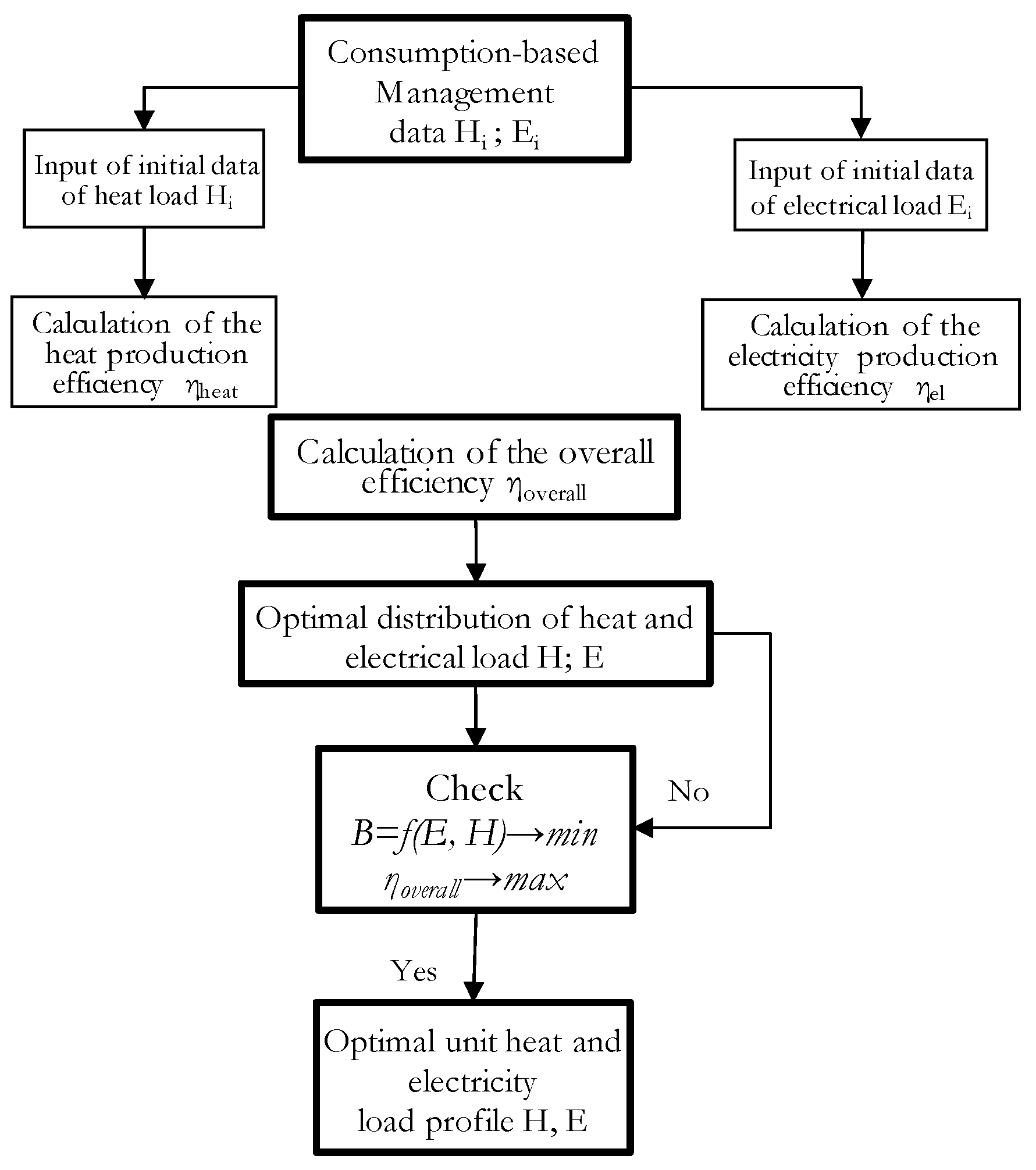
In accordance with the above methodology, we can determine the energy efficiency of a CHP plant based on the demand-side management algorithm of a heating network. The algorithm is shown in Figure 5. Based on the consumption data, we then determine the electrical loads. We then input the data on the current distribution of the generation of heat and electrical loads. Based on the loaded data of the current operating mode of the CHP, we can calculate the efficiency of heat and electricity generation.
The data from the graphs of the electrical and thermal loads of the CHP plant is entered into the model and the efficiency is calculated in the case there is a transition to a new electricity supply mode in accordance with the provision of heating network modes. The optimal operating mode of the power unit and effective redistribution of loads are determined, and, if necessary, further data are gathered on the optimised operating mode of the heating network, which is then used to calculate and select the optimal mode of the future load. The introduction of the structure for optimising energy production at CHP plants will ensure competent and correct decision-making by the CHP personnel concerning technical, economic, and organisational aspects related to the efficient management of heat and electrical equipment.
Let us consider the unit’s consumption of primary energy B, since primary energy is converted into electrical energy E and into thermal energy of a different potential: B = B (E, H), where the increment in the primary energy consumption per unit associated with the change in the unit load can be represented as
d B = B E d E + B H d H
Then, add the total differential (3) in
d B = p ( d E υ + d H )
p = B H  
υ = B E B H
Physically, the coefficient p represents the response of the power unit in terms of primary energy consumption to a change in heat supply to consumers while maintaining the electrical load, and the coefficient υ characterises the relative efficiency of heat supply to consumers compared to the supply of electricity. Let us find the coefficient υ, considering the two variants of the transient process in the system at Ei, Hi, and Bi in the initial state, and Ei, Hji in the final state as a sequence of two transitions:
-
I. Changing H from HiHji while maintaining Bi;
-
II. Changing the electrical power to the initial Ei.
Let us analyse a direct relationship between electric and thermal power and the use of primary energy:
η i = E i + H i B i · Q f
where Qf is the calorific value of the primary energy (fuel).
In the first variant of the transient process (I), the utilisation factor of the primary energy of the power unit changes to a value of ηii in accordance with the change in Ei and Hi after the transition to the load Hji.
η j i = E i + ( H i H j i ) · υ + H j i B i · Q f
where Hi is the thermal power in the initial mode with electric power Ei and the efficiency value ηi, Hji is the thermal power in the current Economic Dispatch mode, and Bi is the primary energy consumption for the initial operating mode.
The result of this optimisation is represented by an objective function that establishes the dependence of efficiency on both heat and electrical loads when operating according to the electrical schedule. When operating on a heating schedule, the electrical power depends on the heat load. The criterion for the optimality of one of the options of the distribution of unit loads at a given value and parameters of the heat supplied is the minimisation of the fuel component considered as the maximum efficiency. The coefficient υ in Equation (8) reflects the efficiency of energy-to-electricity conversion in the CHP unit for a specific change in heat load based on Economic Dispatch.
From Equations (7) and (8) we get:
η j i = η i · ( 1 Δ H i E i + H i · ( υ 1 ) ) = η i Δ H i B i · Q f · ( υ 1 )
where ΔHi = HjiHi. Additionally, let us consider the relationship between the parameters:
η i j η i = b Δ H i · η B
where b is a constant characteristic of a given power unit that does not depend on E, H, or υ.
In the second variant of the transient process (II), the electric power Ei + (HiHji)·υ is restored to the initial value Ei by changing the primary energy consumption from Bi to Bji.
As a result of transformations of Equations (9) and (10), we get a ratio for determining the change in efficiency Equation (11), i.e., primary energy consumption ΔB at ΔHi and E = const:
Δ B Δ H i = 1 E i + H i B i + 1 υ b
The average value of the coefficient p = B H i , where Ei = const for an arbitrary range of heat loads, can be represented as:
p = [ E i + H i B i + 1 υ b ] 1
The coefficient p in Equation (12) corresponds to the new state of heat supply, which led to an increase in ΔHi.
In the initial mode (before the application of Economic Dispatch), the electrical Ei and thermal Hi power correspond to the initial value of the operating efficiency, and when switching to a new load from Equation (3), we get:
B j i B i = p × [ E j i + E i υ + H j i H i ]
Let us determine the coefficient p using the parameters of the initial mode and Equation (13) for this mode:
p = B j i B i E j i E i υ + ( H j i H i )
The coefficient p is determined by two ratios, Equations (14) and (12), describing the transition process from the original mode to the Economic Dispatch mode:
p = 1 [ E j i + H j i B j i + 1 υ b ]
The above method for determining the unit’s consumption of primary energy B makes it possible to change the practical approach to using the efficiency characteristics of CHPs in managing the equipment operating modes and, using the Bji parameter, create a simplified characteristic with qualitative information on the efficiency of the planned heat and electricity generation modes at the CHP.

2.4. Economic Dispatch

Economic Dispatch is a nonlinear optimisation problem with several constraints. The objective function is to minimise the total primary energy consumption with constraints, or in other words, to maximise the overall efficiency. The consumption characteristic curve is a functional dependence of the hourly consumption of primary energy on electric power for various heat loads. We must also consider the minimum and maximum limits for electrical loads as constraints that are determined by technical conditions for different heat loads.
From a mathematical point of view, the problem of Economic Dispatch can be formulated concisely. That is, the objective function, B, must be equal to the overall energy efficiency to supply the indicated heat and electrical load.
The main demand characteristic for a unit on the market is the relationship between primary energy consumption Bi and electrical and thermal power Ei; Hi is a characteristic of consumption or efficiency. The objective function of the problem of short-term optimisation of the CHP operation has the optimisation horizon n = 24 (one day), discreteness Δi = 1 (one hour), and time stamps i. Essentially, the dispatch problem can be formulated as an optimisation problem with a quadratic objective function and linear constraints. The challenge is to find the heat and power generation for each hour so that the objective function defined by the equation is a quadratic polynomial:
B j i = i = 1 n B i = i = 1 n α i   + β i B i + γ i B i 2
where αi, βi, and γi are constant regression equations for hour i. Generation output should be placed between the maximum and minimum limits according to heat production. The corresponding inequality constraints for each generator are.
Ei,minEiEi,max where, Ei,min and Ei,max are the minimum and maximum power output limits of electrical capacity (MW). In order to establish the necessary conditions for the extreme value of the objective function, add the constraint function to the objective function after the constraint function has been multiplied by an undetermined multiplier.
Various methods are used both individually and in combination to optimise power dispatch. These methods include the Lagrange method, the lambda(λ) iteration method, the first- and second-order gradient methods, coefficients of sharing, linear programming, neural networks, and fuzzy algorithms. This model is based on the Lagrange method because it offers an accurate, reliable, and conclusive solution. Compared to other methods, the convergence rate for this model is acceptable. All of this makes it a suitable choice for solving the problems of Economic Dispatch.
The above constrained optimisation problem is converted into an unconstrained optimisation problem. The Lagrange multiplier is used when a function is minimised (or maximised) with a side condition in the form of equality constraints. In this method, the Lagrangian function is formed by adding equality constraints to the objective function using the appropriate Lagrangian multipliers. Using this method, the augmented function is defined as:
L = B i   + λ   ( B j i i = 1 n B i )
Thus, the Lagrange multiplier λ is the cost of one extra MW with an optimal solution. The necessary conditions for the extreme value of the objective function are obtained when we take the first derivative of the Lagrangian function with respect to each of the independent variables and set the derivatives to zero. Now, this Lagrangian function needs to be minimised without any constraints.
To find the minimum, the function with the constraint in the form of Equation (17) is differentiated with respect to all variables (n + 1), and then its derivatives are equated to zero. The minimum of this unconstrained function is at the point where the partials of the function to its variables are equal to zero:
{ L B i = d B j i d B i λ = 0 ; L B i = 0 L λ = 0
The first condition given
L B i = 0 ,   results   in   B j i B i + λ   ( 0 1 ) = 0  
therefore, the mathematically obtained condition for economic dispatch is:
B j i B i = λ
or
β i + 2 γ i B i = λ  
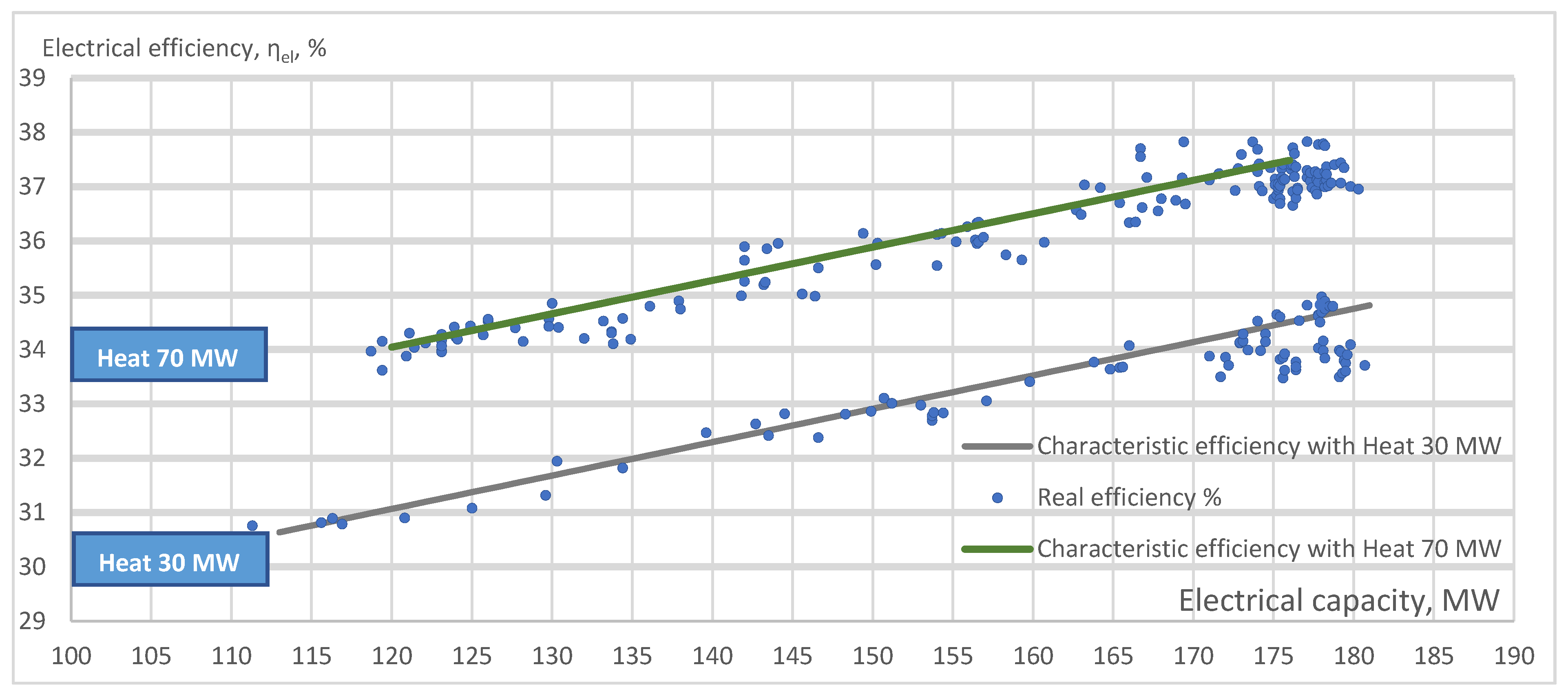
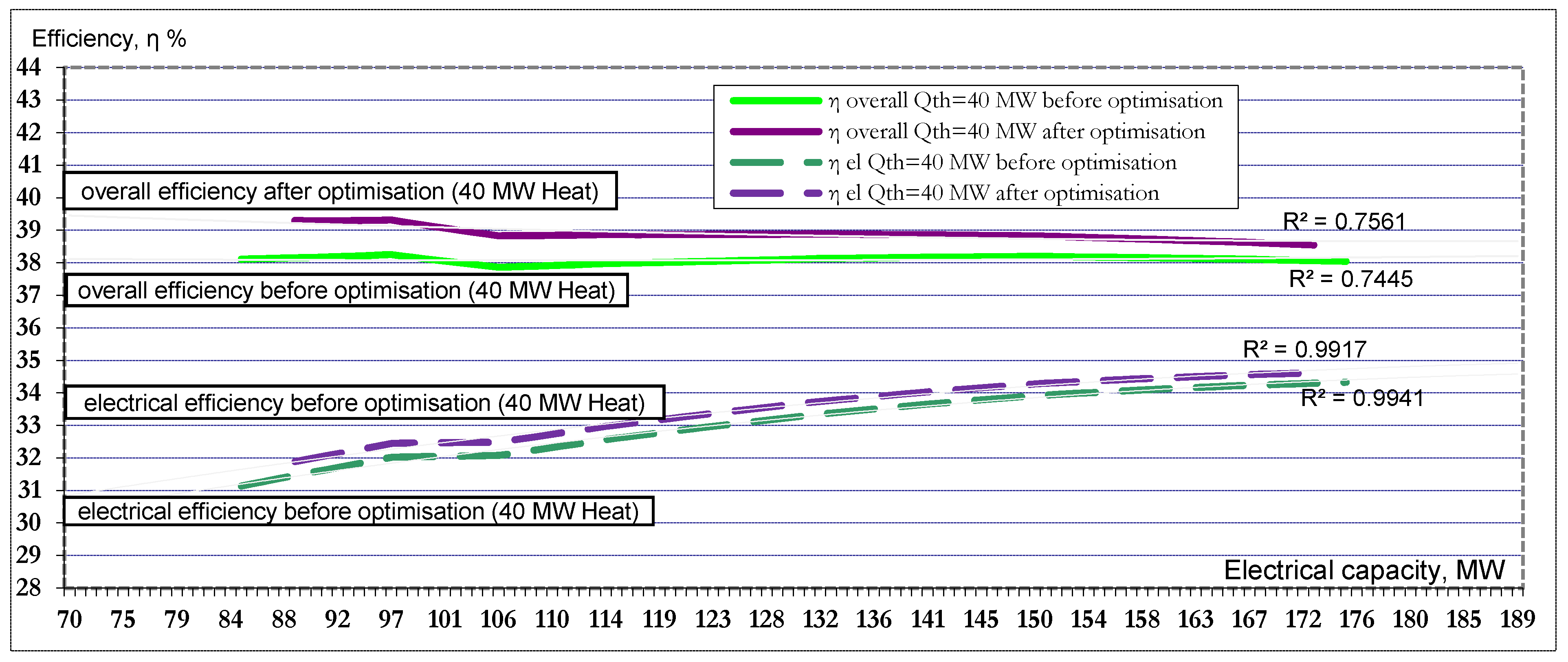
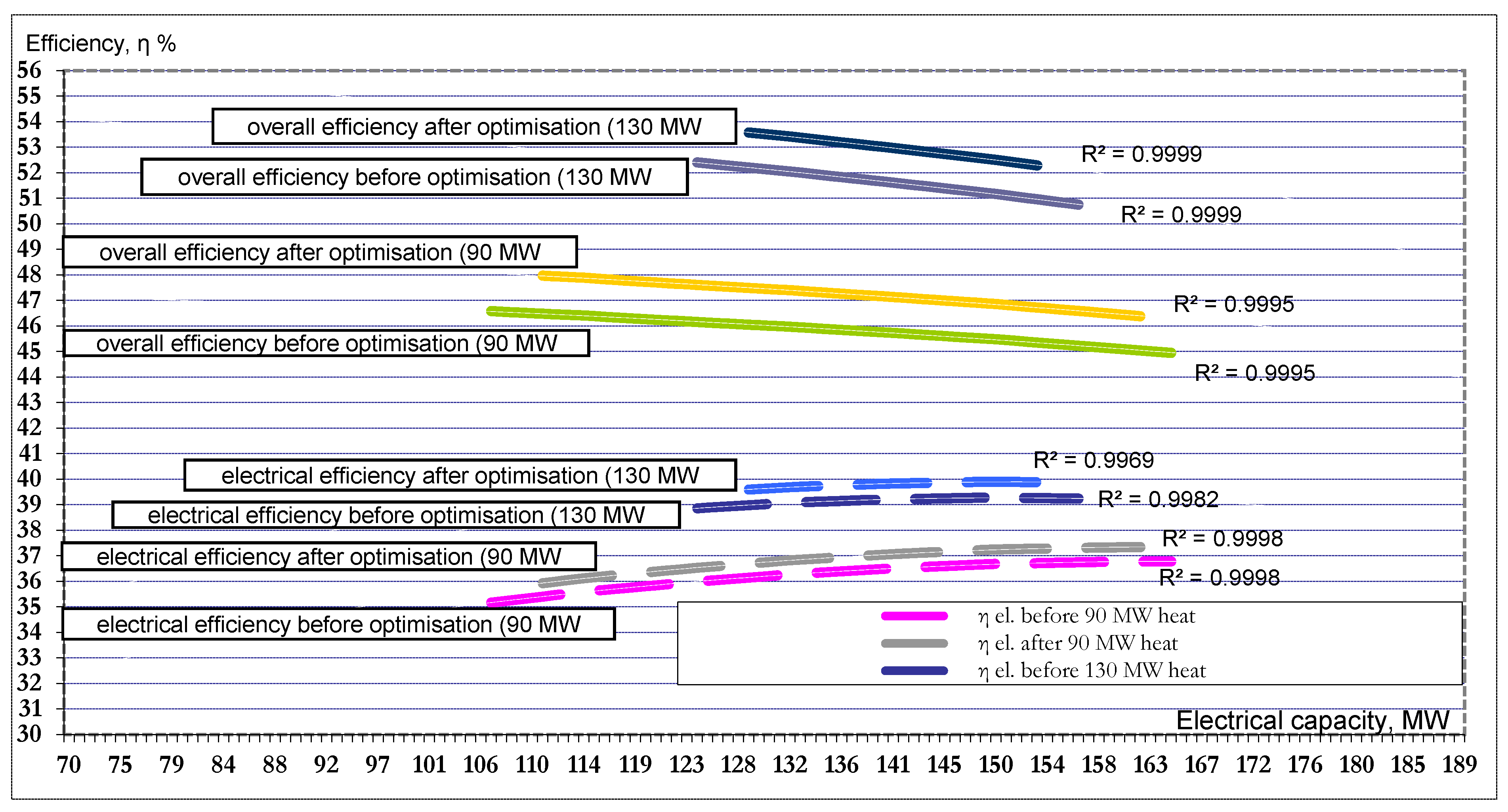
The linearized characteristic of the power unit is a straight-line segment in a two-dimensional regime space for various heat loads. The minimum and maximum electric power, Emin and Emax, (the beginning and end of the straight-line segment), set the power unit control range. The linear functions of electrical efficiency are shown graphically in Figure 6.
Thus, the necessary condition for the existence of the maximum efficiency operating condition for the CHP unit is that the incremental cost rates for the entire capacity must be equal to some undetermined value λ. Of course, to this necessary condition, we must add the constraint equation, according to which the sum of the power outputs must be equal to the power required by the load.
{ B j i B i = λ   for   E i , m i n < E i < E i , m a x ;   B j i B i < λ   for   E i = E i , m a x C B j i B i > λ   for   E i = E i , m i n
The expression β i + 2 γ i B i is the incremental production efficiency of hour i. When solving economic dispatch, the incremental production efficiency of each hour is equal to the Lagrangian parameter λ;. The most economical option is to operate at equal incremental production costs, which can be found as follows:
B i = λ β i 2 γ i
These inequalities indicate that any capacity with an incremental cost higher than λ is inefficient and should operate at the lowest level of capacity.
On the other hand, for each heat load, it is necessary to calculate the incremental costs at the maximum and minimum output for the heat load. Then, set λmin to the smallest value among the incremental costs at unit Emin values, and then set λmax to the largest value among the incremental costs at unit Emax values. If λ = λmin, then the lambda search algorithm is E = Emin, and if λ = λmax, then the lambda search algorithm is E = Emax.
Δ λ = λ m a x λ m i n 2
If the value λ is less than the incremental cost at Emin, then just set the unit output to Emin, and if the value λ is greater than the incremental cost at Emax, then set the generator output to Emax. Otherwise, calculate the E value for the unit from the incremental cost function. A simple procedure to allow the unit to generate B(E) consists of adjusting λ from λmin to λmax in specified increments, where:
λ m i n = m i n ( B i E i ) ;   λ m a x = m a x ( B i E i )     i   for   each   Heat   demand
At each increment, calculate the total primary energy consumption and the total power output for all heat loads. These points represent the points on the B(E) curve or efficiency curve. The incremental cost is the cost of one additional MW per hour. This equality means that the best distribution is achieved in the case of an increase in the primary energy consumption 𝑑Bi with an increase in power 𝑑Ei. Expression (25) determines the order of distribution of heat and electrical loads at the CHP. Thus, the order of priority of electric power is determined by the principle of equality of relative gains; if equality is unattainable, then we use the order of increasing relative gains.

3. Discussion

The district heating network and CHP plant considered in this analysis were based on an actual district heating network located in Narva, Estonia [23] and the Balti Power Plant CHP unit that supplies heat to the Narva DH network. The CHP unit with an extraction-condensing turbine at the Balti Power Plant produces heat and electricity [28]. Figure 7 shows the actual average relationship between thermal and electrical power for the CHP of Narva city during the past five years. This relationship is used for further calculations. As can be seen from the figure, in the operating range of powers, this dependence can be approximated by a linear function with sufficiently high accuracy.
The actual operating data of the CHP unit in September-November 2020 at the minimal thermal loads of 30–70 MW confirm the statistical and calculated characteristics of the unit. The calculations in this paper are based on these data and are shown in Figure 8.
The overall efficiency of a CHP unit refers to the sum of electricity production and useful heat output divided by the amount of fuel used to generate heat in the cogeneration process. The total production efficiency for the scheduled period is the sum of electricity and heat efficiency. In general, the problem of overall efficiency is given as follows:
(1) Maximising the overall operating efficiency of the CHP unit:
η o v e r a l l ( P i ) = i = 1 n   ( η E i + η H i )
where ηoverall is the overall efficiency of the CHP unit; ηEi is the efficiency of electricity production of the CHP unit at hour i; ηHi is heat production efficiency of the CHP unit at hour i; n is the total number of hours.
Let us note the key feature of the cogeneration technology for the generation of electrical and thermal energy, namely the fact that in this case, the physical meaning has a general (overall) efficiency. (ηoverall)—the use of the fuel’s primary energy. The value of the overall efficiency depends on the share of the types of energy generated during cogeneration in their total dimension. The values within which the value (ηoverall) can vary depending on the operating mode of the cogeneration plant. Typical limiting modes include (a) the mode with minimum heat production and maximum electricity generation, with efficiency at the minimum value (ηmin) and (b) the mode with minimum electricity generation and maximum heat production, with efficiency at the maximum value (ηmax).
The qualitative dependence of the change in overall efficiency on the change in heat load is shown in Figure 9.
Hourly system balance. The total heat generation must be equal to the heat load demand, HD, at all hours.
(2) Heat demand balance constraint:
x = 1 n ( H i ) = H D
where Hi is the heat load demand at hour i.
(3) The minimum and maximum rated capacities of the unit must not be violated:
E i ,   m i n E i E i ,   m a x
where Ei, min and Ei, max are the minimum and maximum electricity capacity according to heat demand.
The efficiency curve of a conventional heating unit can be approximated by a quadratic function. A CHP unit has a convex cost function for both power and heat. The bi-objective economic dispatch problem is converted into a single optimisation problem by introducing the maximum overall efficiency as follows:
max   η   o v e r a l l = ( η E i ( a i P i 2 + b i P i + c i ) + η H i ( d i P i 2 + e i P i + f i ) )
-Electricity production efficiency per hour at maximum power output is determined as
η E i ( P E i ( max ) ) = a i P E i ( max ) 2 + b i P E i ( max ) + c i
-Heat production efficiency per hour at demand supply is determined as
η H i ( P H i ( d e m a n d ) ) = d i P H i ( d e m a n d ) 2 + e i P H i ( d e m a n d ) + f i
The operating efficiency determined by the above quadratic Equation (32) is obtained by approximating the power in MW. The incremental efficiency is then calculated as
d η E i d P E i = a i P E i + b i   and   d η H i d P H i = d i P H i + e i

4. Study Results

4.1. Comparison at the Minimum Heat Load of the Heating Network

In the first stage of calculations, the optimisation criterion is the maximum generation of electrical power in terms of heat consumption. Based on statistical data, a regression model has been built, reflecting the dependence of the efficiency of power generation and the overall efficiency of the CHP unit with a minimum heat load of 40 MW (Figure 10).
The CHP unit is loaded more optimally, which increases the efficiency of electricity up to 0.5%, and the overall efficiency of the unit up to an additional 1.0% with a heat supply of 40 MW. A statistical relationship was found between the efficiency of electricity generation by CHPs and a fixed minimum supply of heat. By differentiating this function, we can find the characteristic of the relative increase in efficiency, which will be about 1%.

4.2. Comparison at the Maximum and Average Heat Load of the Heating Network

Based on statistical data, a regression model has been built that reflects the dependence of the efficiency of power generation and the overall efficiency of the CHP unit with an average heat load of about 90 MW, and a maximum heat load of 130 MW. A similar calculation based on statistical data was used to build a regression model that reflects the dependence of the efficiency of power generation and the overall efficiency of the CHP unit with a heat load of 90 MW and 130 MW (Figure 11).
One can observe that with a clear reflection of the heat load, based on the demand data, the CHP unit is loaded more optimally, which increases the efficiency of power generation by about 0.7%, and the overall efficiency of the unit up to an additional 1.5% with a heat supply of 90 MW. It should be noted that heat release was recorded to depict the dependency, which greatly simplified the construction and search for a statistical model, and as a result, it was possible to find a sufficiently high-quality characteristic showing that with a clear reflection of the heat load, based on the demand data, the CHP unit is loaded more optimally, which increases the efficiency of electricity by up to 1.0%, and the overall efficiency of the unit up to an additional 2.0% with a heat supply of 130 MW.

4.3. Summary

From the viewpoint of power unit loading in the wholesale market, this optimisation can be interpreted in such a way that the power unit loading is advisable as long as the relative increase in the cost of electricity generation at the power plant is lower than the market price at which the additional generation is sold, and only then the power plant obtains the maximum economic effect from operating in the wholesale market. A similar effect can be achieved if the price offer on the market matches the relative increase in production efficiency.
Thus, an error in heat supply forecast can lead either to an unreasonably high load of the power plant and sales at a price below the relative increase in the cost of fuel equivalent consumption, or to underutilisation of capacities and a decrease in electricity sales.
However, in most cases, statistical data do not allow for obtaining probabilistic models of characteristics and influencing factors; therefore, the most realistic is the use of heat demand-side management.
At the same time, under conditions of uncertainty, predicting these characteristics is a rather difficult task, which can lead to lost profits when operating on the open electricity market. In particular, the heat supply mode significantly affects the characteristics of the CHP unit.

5. Conclusions

5.1. Summary Model Validation

When distributing the CHP unit load using heat demand-side management, optimisation tasks were formulated, namely the minimisation of primary energy consumption and maximisation of the total useful electrical load of the CHP unit at a given electrical load of the unit and at a given heat load of consumers.
A method based on DH demand data was proposed to optimise the operation of a cogeneration plant and to determine the energy savings of the primary fuel and/or an increase in the efficiency during the cogeneration of electric and thermal energy compared to the traditional method.
The methodology is based on an analytical expression that determines the dependence of the consumption of thermal energy of the primary fuel for the production of electrical and thermal energy during the cogeneration process, taking into account the corresponding efficiency values.
The use of the proposed method was illustrated by an example that shows that the maximum effect of primary energy savings during the cogeneration of electrical and thermal energy under the assumed design conditions is about 2%, compared to the energy consumption of primary fuel for the production of the same amount of electrical energy and thermal energy using the traditional production planning method.
The results obtained and the analysis performed indicate that the proposed methodology provides logical results and can be used to calculate the efficiency indicators of the cogeneration of electrical and thermal energy.

5.2. Summary Calculation Results

The analysis of the calculation results showed that with more optimal planning of a portion of the load at the CHP, the primary energy savings for the heating period due to the difference in the efficiency of the supply will be about 10,000 MWh per year. In addition, fuel savings for the heating season will reach around 18,000 tons of CO2 per year. The results obtained can be used to increase the effect of energy saving measures and to optimise the operation of the CHP system.
Simulating a real CHP unit with a district heating network shows that demand-side management can improve the overall economic efficiency of the CHP plant and increase the unit’s operating range.
As a result, the problem of optimising the operating mode of the CHP unit was solved, which allows us to determine the optimal additional increase in the unit’s electrical load at a given heat load of consumers, which, on average, increases the CHP unit’s efficiency up to an additional 1.5%.

5.3. Summary Study Result

The practical value of the work is experimental calculations on the data of the CHP unit of the Balti Power Plant—showed the practical suitability of the developed tools. The results obtained served as effective information support and can be used to substantiate the distribution of heat and electric energy at CHPs.
In conclusion, it should be noted that the format of this research did not permit a discussion of all the problems of CHP units that arise when operating in the wholesale electricity market, for example, the issue of forced generation at minimum loads, the problem of accounting for the need to turn on peak hot water boilers to ensure electrical generation, and so on. However, these problems should be the subject of a separate discussion and solutions.

Author Contributions

Conceptualization, P.R. and A.V.; methodology, A.V. and P.R.; software, K.L.; validation, A.S. and P.R.; investigation, P.R. and A.S.; writing—original draft preparation, P.R.; writing—review and editing, P.R. and A.V.; visualization, K.L.; supervision, A.V.; project administration, A.S. All authors have read and agreed to the published version of the manuscript.

Funding

This research received no external funding.

Institutional Review Board Statement

Not applicable.

Data Availability Statement

Data was obtained from Narva Soojusvõrk AS and are available from the authors with the permission of Narva Soojusvõrk AS.

Conflicts of Interest

The authors declare no conflict of interest.

Nomenclature

Abbreviation
CHPcombined heat and power
EDeconomic dispatch
DHdistrict heating
DHNdistrict heating network
DSMdemand-side management
Parameters
Hheat, MW
Qheat supply, MW
Bprimary energy (fuel heat), MW
Eelectrical energy, MW
Cunit production cost function
LLagrange function
ηefficiency, %
λLagrange multiplier
υcoefficient of relative efficiency of heat.
pcoefficient of primary energy rate of heat
ttemperature, °C
Ttime period
xheat user
yheat source
mflow rate, kg/h
cspecific heat of water 4,19 kJ/(kg °C)
n24 h—one day
itime stamps Δi = 1 one hour
Subscripts
a, b, celectrical efficiency coefficients
d, e, fheat efficiency coefficients
α, β, γunit efficiency coefficients
1supply
2return
minminimum
maxmaximum
iinitial state
iicurrent state

References

  1. Vanhoudt, D.; Claessens, B.; Salenbien, R.; Desmedt, J. The use of distributed thermal storage in district heating grids for demand side management. arXiv 2017, arXiv:abs/1702.06005. [Google Scholar]
  2. Nazari-Heris, M.; Mohammadi-Ivatloo, B.; Asadi, S.; Geem, Z.W. Large-scale combined heat and power economic dispatch using a novel multi-player harmony search method. Appl. Therm. Eng. 2019, 154, 493–504. [Google Scholar] [CrossRef]
  3. Lutsch, T.; Gampe, U.; Buchheim, G. Steam Injected Gas Turbine (STIG) for Load Flexible CHP: Aspects of Dynamic Behaviour, Control and Water Recovery GT2019-90748; ASME: Phoenix, AZ, USA, 2019. [Google Scholar] [CrossRef]
  4. Kazda, K.; Li, X. A critical review of the modeling and optimization of combined heat and power dispatch. Processes 2020, 8, 441. [Google Scholar] [CrossRef] [Green Version]
  5. Srivastava, A.; Das, D.K. A new Kho-Kho optimization Algorithm: An application to solve combined emission economic dispatch and combined heat and power economic dispatch problem. Eng. Appl. Artif. Intell. 2020, 94, 103763. [Google Scholar] [CrossRef]
  6. Ommen, T.; Markussen, W.B.; Elmegaard, B. Comparison of linear, mixed integer and non-linear programming methods in energy system dispatch modelling. Energy 2014, 74, 109–118. [Google Scholar] [CrossRef]
  7. Wang, J.; You, S.; Zong, Y.; Cai, H.; Træholt, C.; Dong, Z.Y. Investigation of real-time flexibility of combined heat and power plants in district heating applications. Appl. Energy 2019, 237, 196–209. [Google Scholar] [CrossRef]
  8. Liu, X.; Wu, J.; Jenkins, N.; Bagdanavicius, A. Combined analysis of electricity and heat networks. Appl. Energy 2016, 162, 1238–1250. [Google Scholar] [CrossRef] [Green Version]
  9. Li, Z.; Wu, W.; Shahidehpour, M.; Wang, J.; Zhang, B. Combined Heat and Power Dispatch Considering Pipeline Energy Storage of District Heating Network. IEEE Trans. Sustain. Energy 2016, 7, 12–22. [Google Scholar] [CrossRef]
  10. Lin, C.; Wu, W.; Zhang, B.; Sun, Y. Decentralized Solution for Combined Heat and Power Dispatch through Benders Decomposition. IEEE Trans. Sustain. Energy 2017, 8, 1361–1372. [Google Scholar] [CrossRef]
  11. Wu, C.; Gu, W.; Jiang, P.; Li, Z.; Cai, H.; Li, B. Combined Economic Dispatch Considering the Time-Delay of District Heating Network and Multi-Regional Indoor Temperature Control. IEEE Trans. Sustain. Energy 2018, 9, 118–127. [Google Scholar] [CrossRef]
  12. Haghrah, A.; Nazari-Heris, M.; Mohammadi-Ivatloo, B. Solving combined heat and power economic dispatch problem using real coded genetic algorithm with improved Mühlenbein mutation. Appl. Therm. Eng. 2016, 99, 465–475. [Google Scholar] [CrossRef]
  13. Vasebi, A.; Fesanghary, M.; Bathaee, S. Combined heat and power economic dispatch by harmony search algorithm. Int. J. Electr. Power Energy Syst. 2007, 29, 713–719. [Google Scholar] [CrossRef]
  14. Wang, L.; Singh, C. Stochastic combined heat and power dispatch based on multi-objective particle swarm optimization. Int. J. Electr. Power Energy Syst. 2008, 30, 226–234. [Google Scholar] [CrossRef]
  15. Wood, A.J.; Wollenberg, B.F.; Sheblé, G.B. Power Generation, Operation, and Control, 4th ed.; John Wiley & Sons: Hoboken, NJ, USA, 2014. [Google Scholar]
  16. Mancarella, P.; Chicco, G. Real-Time Demand Response From Energy Shifting in Distributed Multi-Generation. IEEE Trans. Smart Grid 2013, 4, 1928–1938. [Google Scholar] [CrossRef]
  17. Nwulu, N. Combined Heat and Power Dynamic Economic Emissions Dispatch with Valve Point Effects and Incentive Based Demand Response Programs. Computation 2020, 8, 101. [Google Scholar] [CrossRef]
  18. Kitapbayev, Y.; Moriarty, J.; Mancarella, P.; Blöchle, M. A real options assessment of operational flexibility in district energy systems. In Proceedings of the 2013 10th International Conference on the European Energy Market (EEM), Stockholm, Sweden, 27–31 May 2013. [Google Scholar] [CrossRef]
  19. Lund, H.; Werner, S.; Wiltshire, R.; Svendsen, S.; Thorsen, J.E.; Hvelplund, F.; Mathiesen, B.V. 4th Generation District Heating (4GDH). Integrating smart thermal grids into future sustainable energy systems. Energy 2014, 68, 1–11. [Google Scholar] [CrossRef]
  20. Volkova, A.; Mašatin, V.; Siirde, A. Methodology for evaluating the transition process dynamics towards 4th generation district heating networks. Energy 2018, 150, 253–261. [Google Scholar] [CrossRef]
  21. Ministry of Economic Affairs and Communications. Analysis of the Technical Feasibility and Cost-Effectiveness of Remotely Read Energy Meters; Ministry of Economic Affairs and Communications: Tallinn, Estonia, 2020. (In Estonian) [Google Scholar]
  22. Rušeljuk, P.; Volkova, A.; Lukić, N.; Lepiksaar, K.; Nikolić, N.; Nešović, A.; Siirde, A. Factors Affecting the Improvement of District Heating. Case Studies of Estonia and Serbia. Environ. Clim. Technol. 2020, 24, 521–533. [Google Scholar] [CrossRef]
  23. Noussan, M.; Jarre, M.; Poggio, A. Real operation data analysis on district heating load patterns. Energy 2017, 129, 70–78. [Google Scholar] [CrossRef] [Green Version]
  24. Volkova, A.; Latõšov, E.; Lepiksaar, K.; Siirde, A. Planning of district heating regions in Estonia. Int. J. Sustain. Energy Plan Manag. 2020, 27, 5–16. [Google Scholar] [CrossRef]
  25. Guelpa, E.; Marincioni, L. Demand side management in district heating systems by innovative control. Energy 2019, 188, 116037. [Google Scholar] [CrossRef]
  26. Guelpa, E.; Marincioni, L.; Deputato, S.; Capone, M.; Amelio, S.; Pochettino, E.; Verda, V. Demand side management in district heating networks: A real application. Energy 2019, 182, 433–442. [Google Scholar] [CrossRef]
  27. Cai, H.; Ziras, C.; You, S.; Li, R.; Honoré, K.; Bindner, H.W. Demand side management in urban district heating networks. Appl. Energy 2018, 230, 506–518. [Google Scholar] [CrossRef]
  28. Wang, D.; Hu, Q.; Jia, H.; Hou, K.; Du, W.; Chen, N.; Wang, X.; Fan, M. Integrated demand response in district electricity-heating network considering double auction retail energy market based on demand-side energy stations. Appl. Energy 2019, 248, 656–678. [Google Scholar] [CrossRef]
  29. Guelpa, E.; Marincioni, L.; Verda, V. Towards 4th generation district heating: Prediction of building thermal load for optimal management. Energy 2019, 171, 510–522. [Google Scholar] [CrossRef]
  30. Verda, V.; Capone, M.; Guelpa, E. Optimal operation of district heating networks through demand response. Int. J. Thermodyn. 2019, 22, 35–43. [Google Scholar] [CrossRef] [Green Version]
  31. Guelpa, E.; Marincioni, L.; Capone, M.; Deputato, S.; Verda, V. Thermal load prediction in district heating systems. Energy 2019, 176, 693–703. [Google Scholar] [CrossRef]
  32. Lepiksaar, K.; Mašatin, V.; Latõšov, E.; Siirde, A.; Volkova, A. Improving CHP flexibility by integrating thermal energy storage and power-to-heat technologies into the energy system. Smart Energy 2021, 2, 100022. [Google Scholar] [CrossRef]
  33. Kurek, T.; Bielecki, A.; Świrski, K.; Wojdan, K.; Guzek, M.; Białek, J.; Brzozowski, R.; Serafin, R. Heat demand forecasting algorithm for a Warsaw district heating network. Energy 2021, 217, 119347. [Google Scholar] [CrossRef]
  34. Saloux, E.; Candanedoa, J. forecasting district heating demand using machine learning algorithms. Energy Procedia 2018, 149, 59–68. [Google Scholar] [CrossRef]
  35. Pihu, T.; Konist, A.; Neshumayev, D.; Loo, L.; Molodtsov, A.; Valtsev, A. Full-scale tests on the co-firing of peat and oil shale in an oil shale fired circulating fluidized bed boiler. Oil Shale 2017, 34, 250. [Google Scholar] [CrossRef]
Figure 1. Narva district heating network.
Energies 14 04553 g001
Figure 2. Dependence of the heat demand on the outdoor air temperature.
Energies 14 04553 g002
Figure 3. Electric and heat load profile before and after economic dispatch according to demand-side management.
Energies 14 04553 g003
Figure 4. Electrical efficiency of the CHP unit based on the heat load.
Energies 14 04553 g004
Figure 5. Flowchart of the application of the demand-side management algorithm to solve the economic dispatch problem of the CHP unit.
Energies 14 04553 g005
Figure 6. Linear function of electrical efficiency based on the heat load.
Energies 14 04553 g006
Figure 7. CHP unit electrical load and heat load according Narva city DH network.
Energies 14 04553 g007
Figure 8. Electrical efficiency of the unit for heat load 30 MW and 70 MW.
Energies 14 04553 g008
Figure 9. Overall and electrical efficiency of the CHP unit based on the heat load.
Energies 14 04553 g009
Figure 10. Efficiency optimisation result for minimum 40 MW heat demand.
Energies 14 04553 g010
Figure 11. Efficiency optimisation result for an average 90 MW and maximum 130 MW heat demand.
Energies 14 04553 g011
Publisher’s Note: MDPI stays neutral with regard to jurisdictional claims in published maps and institutional affiliations.

