Article

Advanced Exergy Analysis of Waste-Based District Heating Options through Case Studies

by
Huseyin Gunhan Ozcan
1,
Arif Hepbasli
1,
Aysegul Abusoglu
2,* and
Amjad Anvari-Moghaddam
3,*
1
Department of Energy Systems Engineering, Yasar University, Bornova, Izmir 35100, Turkey
2
Department of Mechanical Engineering, Istanbul Technical University, Istanbul 34437, Turkey
3
Integrated Energy Systems Laboratory, Department of Energy (AAU Energy), Aalborg University, 9220 Aalborg, Denmark
*
Authors to whom correspondence should be addressed.
Energies 2021, 14(16), 4766; https://doi.org/10.3390/en14164766
Submission received: 9 July 2021 / Revised: 30 July 2021 / Accepted: 2 August 2021 / Published: 5 August 2021
(This article belongs to the Special Issue Energy and Exergy Analysis of Renewable Energy Conversion Systems)

Abstract

:
The heating of the buildings, together with domestic hot water generation, is responsible for half of the total generated heating energy, which consumes half of the final energy demand. Meanwhile, district heating systems are a powerful option to meet this demand, with their significant potential and the experience accumulated over many years. The work described here deals with the conventional and advanced exergy performance assessments of the district heating system, using four different waste heat sources by the exhaust gas potentials of the selected plants (municipal solid waste cogeneration, thermal power, wastewater treatment, and cement production), with the real-time data group based on numerical investigations. The simulated results based on conventional exergy analysis revealed that the priority should be given to heat exchanger (HE)-I, with exergy efficiency values from 0.39 to 0.58, followed by HE-II and the pump with those from 0.48 to 0.78 and from 0.81 to 0.82, respectively. On the other hand, the simulated results based on advanced exergy analysis indicated that the exergy destruction was mostly avoidable for the pump (78.32–78.56%) and mostly unavoidable for the heat exchangers (66.61–97.13%). Meanwhile, the exergy destruction was determined to be mainly originated from the component itself (endogenous), for the pump (97.50–99.45%) and heat exchangers (69.80–91.97%). When the real-time implementation was considered, the functional exergy efficiency of the entire system was obtained to be linearly and inversely proportional to the pipeline length and the average ambient temperature, respectively.

Graphical Abstract

1. Introduction

District heating (DH) is not a new technology. It is a technology that has evolved considerably over the last four decades. During the 1980s, the essential characteristics of networks were the main research focus. During the next decade, DH was integrated into many modern societies in Europe and North America. During the early 21st century, sustainable systems, with lesser carbon emissions, have become the focal point. Over the last couple of years, scientific studies have focused on a more integrated and large-scale approach [1].
DH also indicates the significant potential and has been well documented. However, it only has, on average, a market share of 10% throughout Europe, while it is mainly restricted to northern and central nations [2,3]. Globally, heating is responsible for half of the final energy demand. Meanwhile, the heating of buildings, together with domestic hot water supply, accounts for almost half of the total generated heating energy (50% in industrial processes, 46% in buildings, and the remainder was used in agriculture, essentially for greenhouse heating). On the other hand, 92% of DH was powered by fossil fuels in 2018. Therefore, increasing the share of renewables and/or waste heat (WH) in DH systems (DHSs) is a crucial factor in achieving the 2030 United Nations sustainable development goals [4].
DHSs mostly have an essential link between facilities generating heat with low exergy content and consumers [5]. Excess heat also exists from many sources, and its avoidance or utilization would cause a reduction in the primary energy use and greenhouse gas emissions that are released during the combustion of fossil fuels [6]. In the process industry, a large amount of WH is usually available. Depending on various temperature levels, industrial WH can be split into low-, medium-, and high-grade WHs. Although there are no clearly defined values for these three levels, 650 °C and 230 °C may be accepted as the dividing points [7,8].
Exergy-based tools have been widely used in analyzing and assessing the performance of energy-related systems in the recent years. These tools can be categorized into conventional and advanced exergy analysis. In the advanced exergy method, one can perform a more comprehensive analysis by investigating and identifying the interactions of sections with each other, in terms of exergy destructions (endogenous/exogenous and unavoidable/avoidable constituents), while the potential for improvements is deducted.
As far as previously conducted studies are concerned, Hepbasli and Keçebaş [9] assessed the performance of a geothermal DHS in Turkey, through conventional and advanced exergetic analysis methods based on real operational data. They reported that the conventional and modified exergetic efficiency values were 29.29% and 34.46%, respectively. These geothermal-based exergetic analyses and assessments were conducted for different Turkish cities, by various investigators, such as Tan and Keçebaş [10] and Yamankaradeniz [11], with an exergo-environmental analysis that was performed by Yürüsoy and Keçebaş [12]. The overall conventional and advanced exergy efficiencies were determined to be 43.72% and 45.06% [10], and 25.24% and 26.34% [11], with exergoeconomic factors of 5.25% and 12.98% [12], respectively. Sangi et al. [13] developed a Modelica-based tool for performing a dynamic exergy analysis of energy systems. This analysis was carried out by two sub-models, the ExergySensor and the ExergyAnalysisTool, while a model of a district in Bottrop, Germany, along with its energy system, was also developed. Koroglu and Sogut [14] considered a steam power plant, to which they applied conventional and advanced exergy analysis methods. They reported that the overall system had a 10% improvement potential of the exergy efficiency. Fellaou and Bounahmidi [15] assessed the performance of a cement plant that was located in Morocco, through conventional and advanced exergetic analyses. They determined that 31.54% of the total exergy destruction in raw mill two was avoidable, followed by 29.21% and 15% in raw mill one and the calciner, respectively. Idrissa and Boulama [16] considered a combined Brayton/Brayton power cycle to assess its performance using advanced exergy analysis. They determined that the largest exergy destruction occurred due to the combustion chamber, followed by the topping cycle turbine, the compressor, and the recovery HE. Fito et al. [17] considered an industrial WH recovery system that was located in DH in Grenoble, France. The 4E analyses, namely, energy, exergy, economic and exergoeconomic analyses, were used to evaluate its performance. Based on source-oriented and demand-oriented optimizations with 40-MWh storage capacity, recovering WH at 85 °C without heat pump and at 35 °C with heat pump configurations were recommended, respectively. Fito et al. [18] also performed energy- and exergy-based comparative analyses of a WH recovery system for DH in optimal design aspects. The energy analysis was based on the heating demand coverage and WH recovered, as two indicators, while the exergy analysis used only one indicator, which was global annual exergy efficiency. The exergy analysis with the highest global exergy efficiency of 27% was in good agreement with the source-oriented design. Pan et al. [19] developed and analyzed a novel organic Rankine cycle (ORC) heat pump system for waste-to-energy, which recovered the WH of low-temperature exhaust gas and ultra-low-temperature WH. A higher electrical efficiency of 28.4% was obtained, with an improvement of 6.5% compared to the conventional system. Allen et al. [20] used energy modeling for comparing the energy performance of conventional and advanced district thermal energy systems at the urban district level. Radiant hydronic heating, ventilation, and air conditioning systems, mated with low-exergy district thermal energy systems, had a source energy use intensity that was 49% lower than that of conventional systems. Ambriz-Diaz et al. [21] evaluated a polygeneration plant operating in a geothermal cascade, using advanced exergy and exergoeconomic analysis methods. They concluded that the polygeneration plant could reach an energy efficiency increase of 1.53%, through improvements to be conducted in the design of the system components. Liao et al. [22] proposed alternative ORC-based combined power systems, and analyzed them using advanced exergy analysis. According to their assessment, the ORC–ORC system, with heptane/R601a as working fluids, had the highest thermal and exergy efficiency values of 16.37% and 45.54%, respectively, compared to ORC-based sCO2 systems. Chen et al. [23] proposed a novel integrated hybrid DHS, which consisted of photovoltaic/thermal collector, absorption, and geothermal heat pump technologies, to produce space heating water for an office building in China. Based on the modified thermo-ecological cost analysis, a 66% photovoltaic coverage ratio of photovoltaic/thermal collector led to a minimum thermo-ecological heating cost of 6.86 J/J. Wang et al. [24] coupled the ORC and the absorption refrigeration, driven by WH, with the CO2 capture and storage process. They analyzed this integrated process through advanced exergy and advanced exergoeconomic analysis methods. The total system exergy efficiency value was determined to be 17.56%, with a total exergy destruction rate of 36,424 kW, of which 43.15%, 32.35%, and 24.50% belonged to the CO2 capture–storage, ORC, and absorption refrigeration cycle processes, respectively. Caglayan and Caliskan [25] evaluated the performance of a cogeneration system that had a turbine unit and spray dryers, used in a ceramic factory through both conventional and advanced exergy analyses, and investigated the effect of varying dead states temperatures on the efficiency. They calculated the values for the maximum exergy efficiency and the destruction rate of the system as 29.85% and 17.81 MW at a dead state temperature of 30 °C, respectively.
Based on the literature review above, DH systems have a remarkable potential in heating applications in which a more integrated and large-scale approach has been preferred recently. In this regard, WH source-driven DH systems have become an effective solution, enabling considerable energy savings and environmental benefits. Nevertheless, exergy-based assessment methods have been powerful tools, by determining the loss in work potential (exergy destruction) and its origin, namely, due to the component itself (endogenous) or other components (exogenous), and can be enhanced (avoidable), or not (unavoidable), considering the up-to-date technological status for a selected system solution. Therefore, this study focused on performing conventional and advanced exergy analyses of a WH source DH system, based on four various case studies. Meanwhile, ambient temperature and the heat loss in the DH network were assessed as critical parameters during the operation of the WH source DH system, where their effects on the exergy performance were studied, based on four different selected sites in Turkey. In this way, this study differs from other studies, by presenting a comprehensive approach by dealing with many aspects. The main objectives of this paper are as follows:
  • Carry out series simulations for evaluating both the conventional and advanced exergy performances of DH systems with various WH sources, based on four different plants. While municipal solid waste cogeneration, thermal power, wastewater treatment, and cement production plants were considered WH sources, HEs, pump, and the whole system were assessed through exergy analyses;
  • Evaluate the conventional exergy performance of the whole system, based on four different locations in Turkey, using a validated mathematical model. The sites were selected by considering degree-day regions and the situation with the highest population density, and the real-time data group validated the mathematical model;
  • Evaluate the conventional exergy performance of the whole system, based on various distances (5 km, 10 km, 15 km, and 20 km) between the WH sources and the dwellings.

2. Description of a DH System Integrated with an Existing WH Sources

In this study, as shown in Figure 1, four different WH sources (three mid-grade, in a range of temperatures between 100 and 370 °C, and a high grade, in a range of temperatures from 370 up to 900 °C) [26] were investigated under DH options, based on case studies. Within this scope, municipal solid waste cogeneration (case one), thermal power (case two), wastewater treatment (case three), and cement production (case four) plants were considered as a WH source, by their exhaust gas potentials, with the real-time data group. As shown in Figure 1, state one presents the WH input of the examined plants, tabulated at the top of the figure. In case one, direct utilization of the exhaust gas of a cogeneration plant that is located in Gaziantep, Turkey, to supply heat for a DH system, was assessed [27]. In Case 2, coal-fired thermal power plants that are located at Soma in Manisa, and Yatağan in Muğla, Turkey, were considered together. The best point for heat extraction in these plants was determined from a cross-over pipe between intermediate and low-pressure turbines for a DH system supply, rather than mechanical energy production close to the condenser [28,29]. While Ref. [28] implies properties of the circulated water between the HEs and the dwellings (states between four and eight), Ref. [29] gives information about the WH side (states one and two, in Figure 1). In case three, the exhaust gas of the biogas engine-driven cogeneration, with the increased power output, using all the biogas produced, was considered, to produce WH in a wastewater treatment plant [30]. In case four, a cement production plant that is located in Gaziantep, Turkey, was studied, and the hot gas exhaust from the raw mill unit that is employed in the cement production process (State 1), was considered [31]. In this case, while the temperatures of the states, except one, were obtained from Ref. [32], considering DH using low-grade industrial waste heat options, the pressures were considered, as in case two. The details of each plant operation can be found in Ref. [27], for municipal solid waste cogeneration, in Refs. [28,29] for thermal power, in Ref. [30] for wastewater treatment, and in Ref. [31] for cement production.
As seen in Figure 1, the WH potential of the examined plants, by extracting exhaust gases (state one), is transferred to the cold water (state four), through the first heat exchanger (HE-I). In this heat exchange process, while the exhaust gas is cooled and discharged into the atmosphere (state two), the water is heated (state three) and transported to the second heat exchanger (HE-II) (state five). In this heat exchange process, while the heated water (state five) is cooled again (state six), the cold water that is taken from the dwellings (state eight) is heated and supplied to the dwellings (state seven). The water is pressurized between the employed HEs with the pump.

3. Description of the Developed Mathematical Model for the Advanced Exergy Assessment

The steady-state simulation model of the four different WH sources, to supply heat for a DH system, was developed using the engineering equation solver (EES), to solve a set of energy and conventional/advanced exergy equations [33]. Within this scope, the thermophysical properties (T, P and m ˙ ) of each state in Figure 1 were defined as known parameters in the written code first. Here, the values in Table 1, which were created based on the real-time data group obtained by Ref. [27], for municipal solid waste cogeneration, by Refs. [28,29] for thermal power, by Ref. [30] for wastewater treatment, and by Ref. [31] for cement production, were used. Next, as in Ref. [27], the dead state values for temperature (T0) and pressure (P0) were assumed as 20 °C and 100 kPa, respectively, for both the working fluids (air and water). These are normal temperature and pressure values, defined by the National Institute of Standards and Technology. The specific enthalpy (h) and specific entropy (s) properties of each state were then calculated using built-in thermophysical property functions. Finally, the specific exergy (ѱ) and exergy rate ( E x ˙ ) of each state were determined using Equations (1) and (2), respectively, considering only the physical part of exergy, in other words neglecting the kinetic, potential, and chemical effects [19].
ψ = h h 0 T 0 · s s 0
E x ˙ = m ˙ · ψ
In Table 2, the h, s and ѱ values are presented.
After finding the exergy rates of each state in the WH source DH system (see Figure 1), the energy performance of the employed components (HE-I, pump, and HE-II) was assessed. The reason for this is that the advanced exergy assessment method covers the definition of the energy performance indicators that belong to each component, regarding the actual, unavoidable and ideal conditions [21]. In this regard, the effectiveness (ε) values were calculated for HE-I and HE-II by Equation (3), based on the effectiveness—number of the thermal unit method [34].
ε = Q ˙ a c t Q ˙ m a x
where Q ˙ a c t and Q ˙ m a x represent the actual and maximum possible heat transfer rate for the considered HEs, respectively. These rates can be evaluated by multiplying the mass flow rates, specific heats and temperature differences of the cold and hot fluids. As for enthalpy and entropy, the specific heats were determined using built-in thermophysical property functions in the written code.
For the pump, isentropic efficiency is used as an energy performance indicator, and is estimated by the following [35]:
η i s = W ˙ i n , i s W ˙ i n , a c t = m ˙ i n * h o u t , i s h i n m ˙ i n * h o u t , a c t h i n = m ˙ i n * v i n * P o u t P i n m ˙ i n * h o u t , a c t h i n
where W ˙ i n , i s and W ˙ i n , a c t indicate the rate of work that is consumed by the pump, in isentropic and actual conditions, respectively. The discrepancy between these two conditions occurs in output specific enthalpies. Under the isentropic pressurized process, the enthalpy difference between the outlet and inlet states can be evaluated by multiplying the specific volume of the inlet state, and the pressure differences between outlet and inlet states [36,37].
After performing energy analysis, conventional exergy analysis was applied to each kth component, based on the fuel (exergy rate of the required resources)–product (exergy rate of the desired output) concept, as shown in Figure 2 [38]. In this concept, the combined effect of the exergy rate from flow (the first two terms), heat transfer (the third term), and work (the last term), within the control volume of each of the kth components (see Equation (5)), was considered. Here, T represents the temperature at which Q ˙ k takes place [39]. As illustrated in Equations (6) and (7), two essential performance indicators, namely, exergy efficiency ( φ k ) and exergy destruction rate ( E x ˙ D , k ), can be derived from Equation (5), for the kth component when exergetic fuel and product rates are well defined [38,39].
E x ˙ F , k E x ˙ P , k = i n · E x ˙ k o u t · E x ˙ k + 1 T 0 T k · Q ˙ k W ˙ k
φ k = E x ˙ P , k / E x ˙ F , k
E x ˙ D , k = E x ˙ F , k E x ˙ P , k
Besides performing the component-based conventional exergy analysis, the functional and overall exergy efficiencies were found for the whole system, by Equations (8) and (9), respectively [40].
φ s y s , f = E x ˙ P , s y s , f E x ˙ F , s y s , f = E x ˙ 7 E x ˙ 8 E x ˙ 1 + W ˙ i n
φ s y s , o = E x ˙ P , k E x ˙ F , k
With the application of advanced exergy analysis, E x ˙ D , k can be divided into unavoidable and avoidable parts, enabling the real improvement potential of the kth component to be obtained. Meanwhile, the interactions between the system components can be defined by finding endogenous and exogenous parts of E x ˙ D , k [38,39]. In this regard, as shown in Figure 2, the EES-based written code was rerun under the unavoidable operating condition of the kth component, together with the actual operating conditions of the remaining ones, to find the ratio of the exergy destruction rate to the product exergy rate in the created unavoidable condition for the kth component E ˙ D , k E ˙ P , k U N . Then, the unavoidable ( E ˙ x D , k U N ) and avoidable ( E ˙ x D , k A V ) splitting parts of the exergy destruction rate can be computed for the kth component, by Equations (10) and (11), respectively [41].
E ˙ x D , k U N = E x ˙ P , k · E ˙ D , k E ˙ P , k U N
E ˙ x D , k A V = E x ˙ D , k E ˙ x D , k U N
Similarly to the unavoidable and avoidable exergy destruction parts, as stated in Figure 2, the EES-based written code was rerun under the actual operating condition of the kth component, together with the ideal operating conditions of the remaining ones, to find the ratio of the exergy destruction rate to the product exergy rate in the created endogenous condition for the kth component E ˙ D , k E ˙ P , k E N . Then, the endogenous ( E ˙ x D , k E N ) and exogenous ( E ˙ x D , k A V ) splitting parts of the exergy destruction rate can be computed for the kth component, by Equations (12) and (13), respectively [41].
E ˙ x D , k E N = E x ˙ P , k · E ˙ D , k E ˙ P , k E N
E ˙ x D , k E X = E x ˙ D , k E ˙ x D , k E N
In the above-given Equations (10)–(13), E x ˙ D , k and E x ˙ P , k are the exergy destruction and product exergy rates of the kth component, respectively, while both are obtained by conventional exergy assessment. Meanwhile, Table 3 lists the actual, unavoidable, and ideal conditions of the four different WH source DH systems, to conduct an advanced exergy assessment. It should be noted here that the EES-based written code provided these conditions by adjusting the thermo-physical properties of the considered states.

4. Results and Discussion

4.1. Model Validation

In this study, the EES package program was used to develop the model of the DH system, utilizing various WH sources, and carry out conventional and advanced exergy analyses. The conventional exergy assessment results of Ref. [27] were used to validate the developed system model working, according to case one. With the same thermo-physical properties of the considered fluids given in Table 1, and under the isentropic efficiency of 94.4% for the pump, the comparison results between the Ref. [27] and simulated values are presented in Table 4. As can be seen from the table, the obtained results for the component-based exergy destruction rates and exergy efficiencies reveal that the simulation model performed with full success in modeling HEs, and the pump having no relative error. However, the functional exergy rate and functional exergy efficiency of the whole system were modeled with 15.5% and 63.8% relative errors, due to different definitions. While Ref. [27] considers states between one and four in Figure 1 to determine these exergy performance indicators, this study focuses on all the states in Figure 1 (from one to eight) to derive equations for the same indicators.

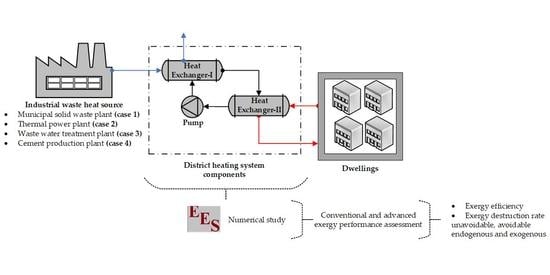
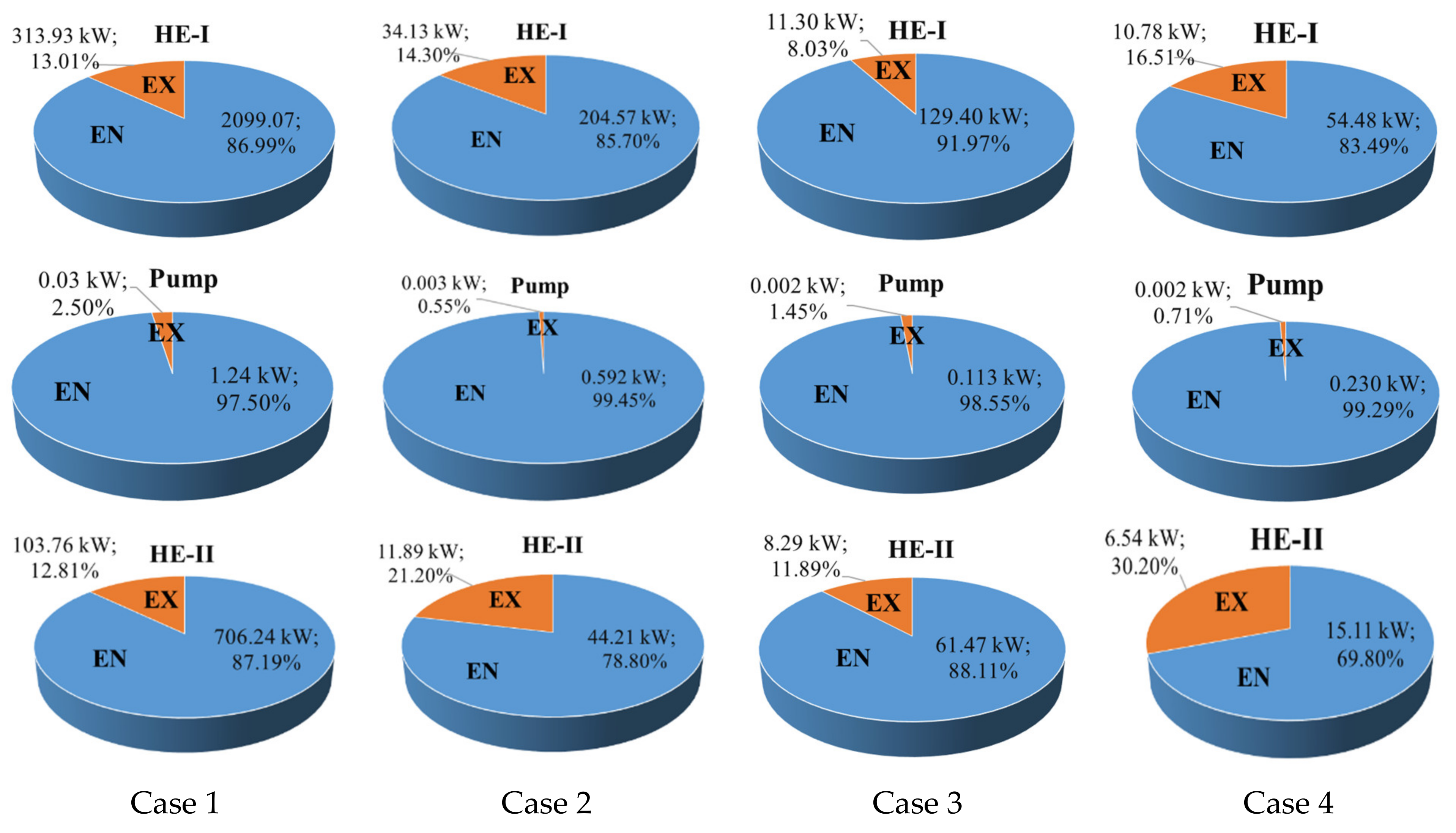
4.2. Exergetic Assessment

In this study, the exergetic performance of the WH source DH system, along with its components, was numerically assessed based on four different cases, through the EES-based written code. In this regard, as presented in 
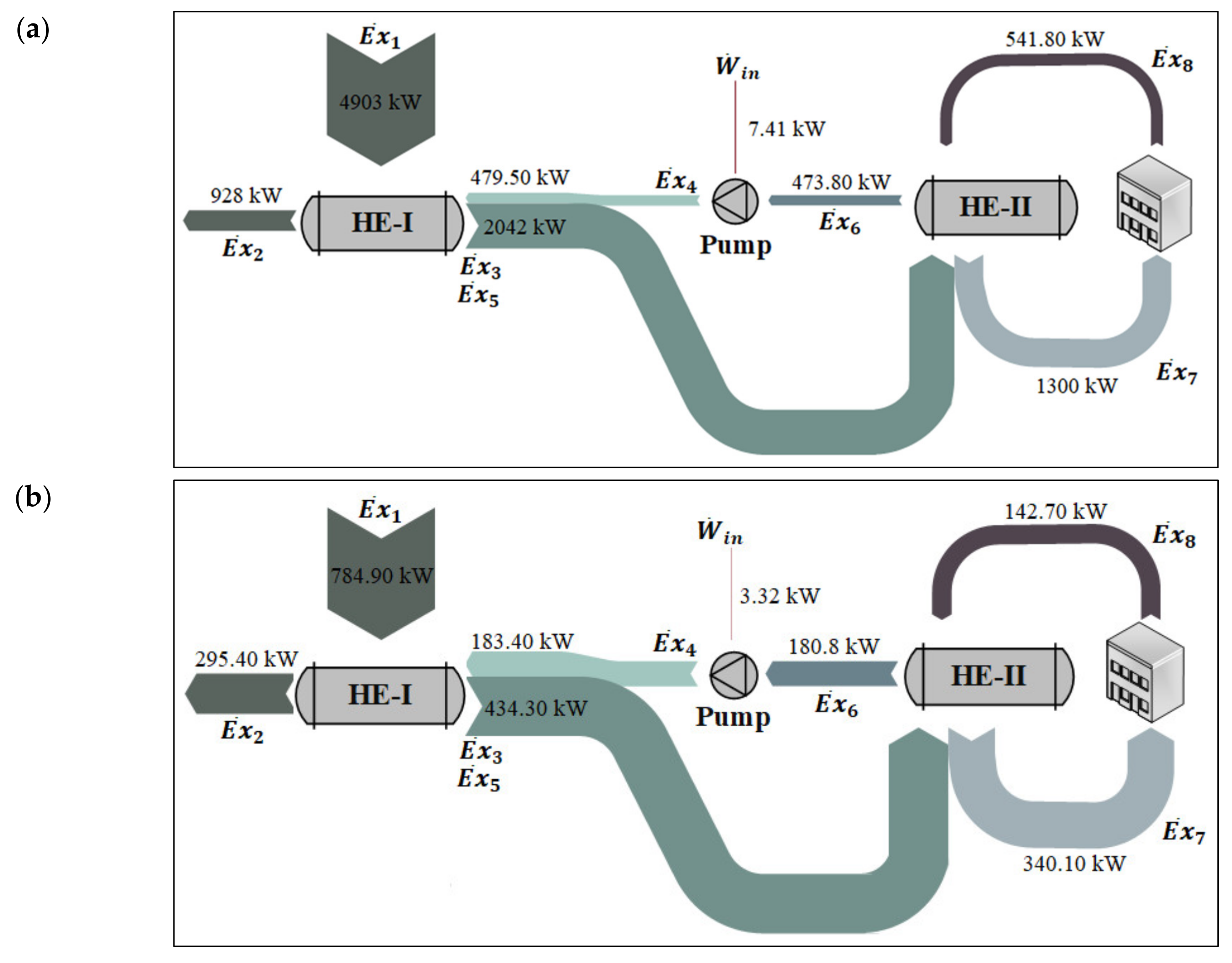
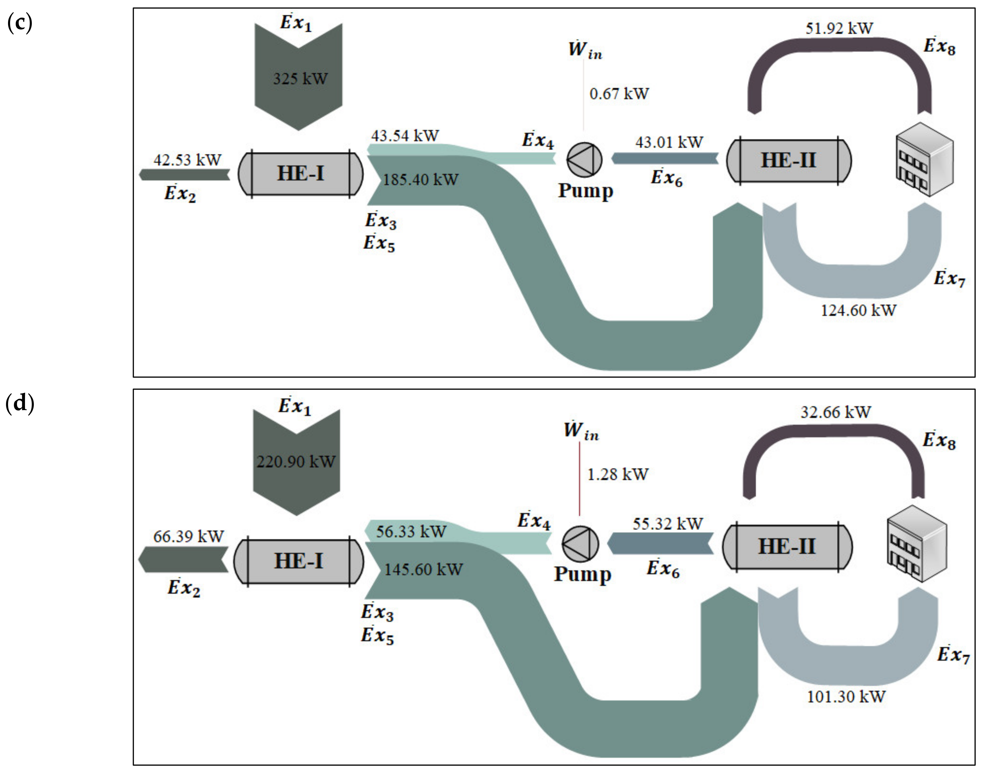
Figure 3a–d, the exergy flows between the main system components were determined by applying the conventional exergy method to the system, based on the created cases one, two, three, and four, respectively. As can be seen in Figure 3, the highest exergy rates were simulated for the WH source ( E x ˙ 1 ), which was as high as 4903 kW (case one) and as low as 220.90 kW (case four). Hereafter, the highest exergy rates were found for the DH network supply ( E x ˙ 3 = E x ˙ 5 ), ranging from 145.60 kW (case four) to 2042 kW (case one). Following the DH network supply, the highest values for the exergy rate were obtained for the water supply to the dwellings ( E x ˙ 7 ), between 101.30 kW (case four) and 1300 kW (case one). On the other hand, the minimum exergy rates were simulated for the work consumption by the pump ( W ˙ i n ), which had its lowest value for case four, with 0.67 kW, and had its highest value for case one, with 7.41 kW. After that, the lowest exergy rates were computed for the DH network return at the pump’s inlet ( E x ˙ 6 ), except case three where the WH source that was discharged into the atmosphere ( E x ˙ 2 ) had the lowest exergy rate after the WH source inlet. Following the DH network return at the inlet of the pump, the lowest values for the exergy rate were obtained for the DH network return at the outlet of the pump ( E x ˙ 4 ), between 43.54 kW (case three) and 479.50 kW (case one).
The obtained results of exergy flow between the main components, based on the created cases given in 
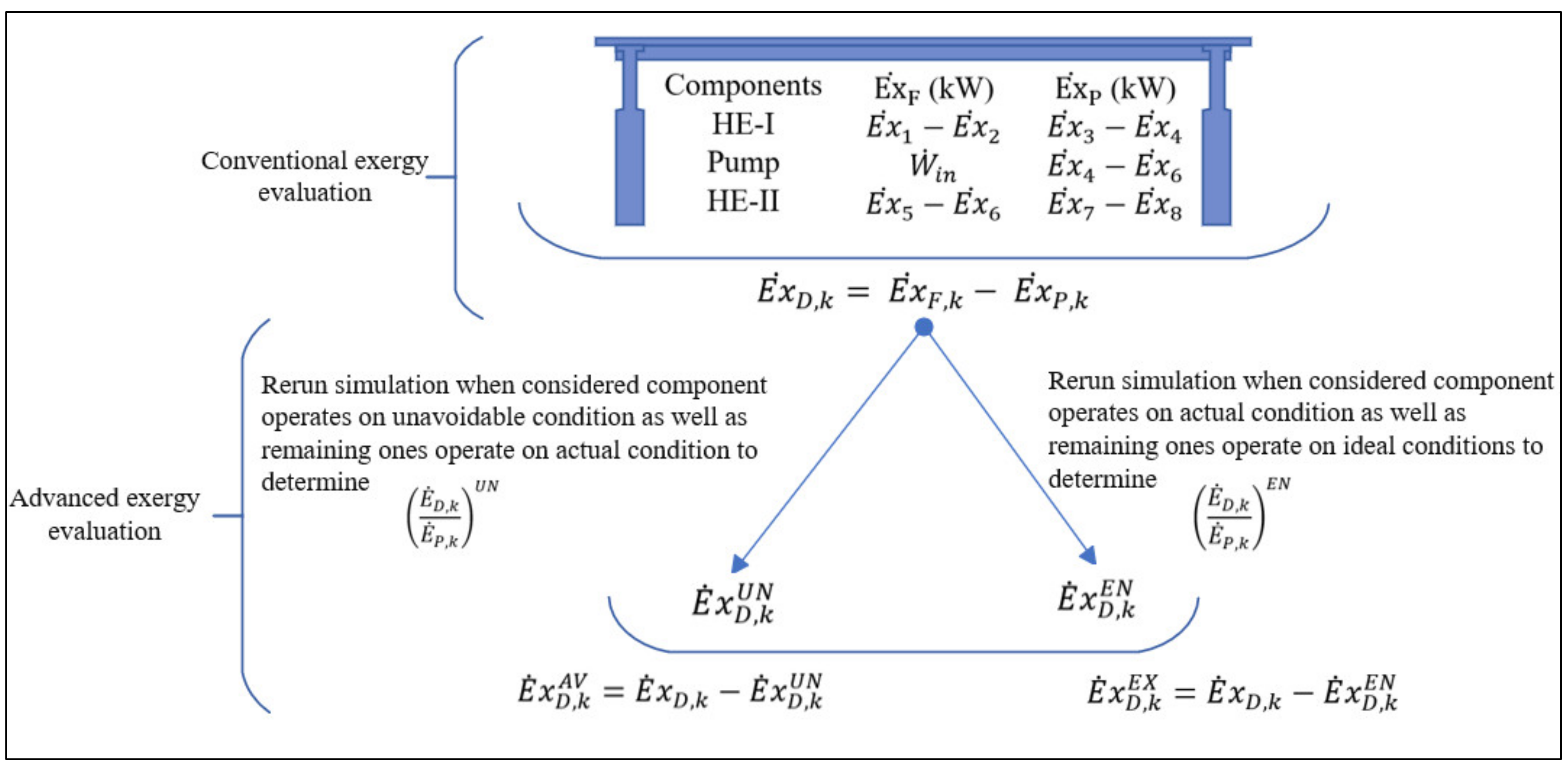
Figure 3, enable the conduction of conventional exergy assessment on a component level (see 
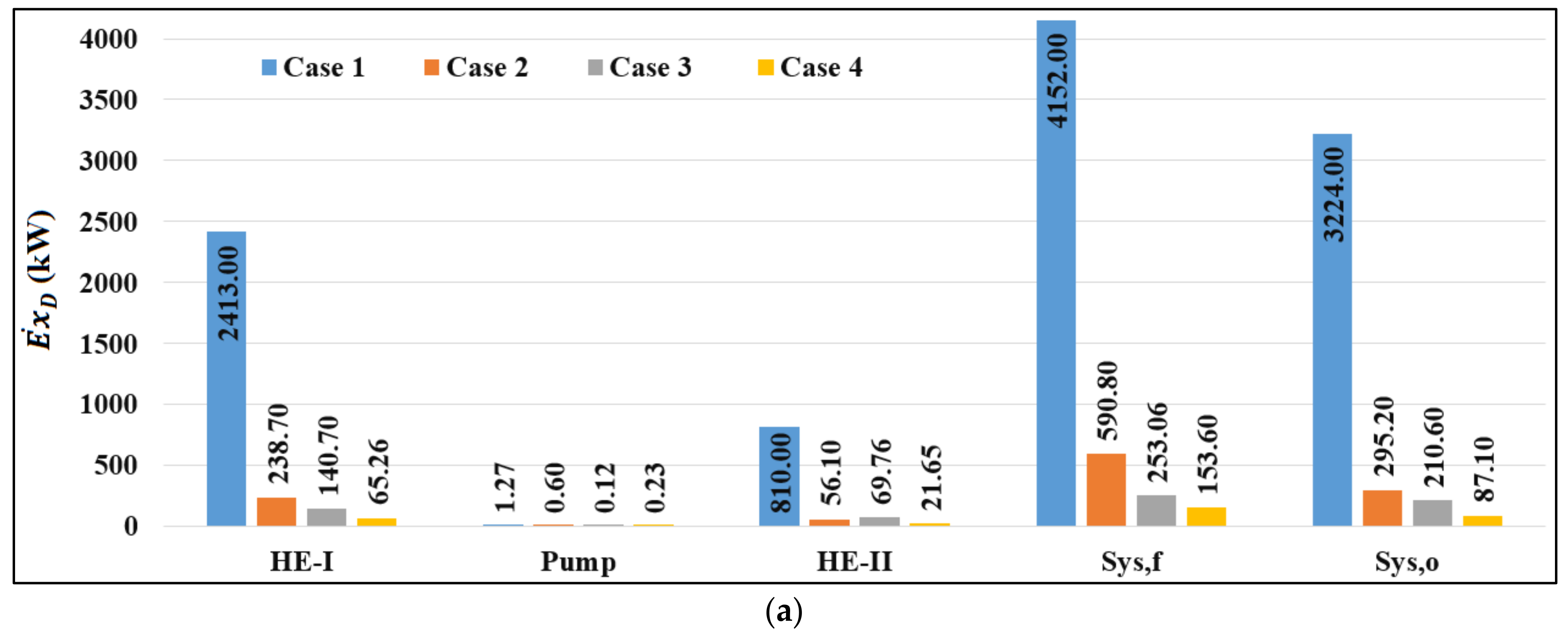
Figure 2) and for the whole system (see Equations (8) and (9)) as well. The simulated results of the performance indicators are presented in Figure 4a,b, respectively, for the exergy destruction rate and exergy efficiency, based on each created case.
As shown in Figure 4a, the exergy destruction rates were computed quite high for the entire system E x ˙ D , s y s , f ,   E x ˙ D , s y s , o and each system component ( E x ˙ D , H E I ,   E x ˙ D , p u m p ,   E x ˙ D , H E I I ) in case one, compared to other cases. The main reason is the high exergy rate of the WH source of this case (see E x ˙ 1 in Figure 3). Meanwhile, as shown in the figure, the exergy destruction rates of the whole system and the component HE-I, change proportionally with the exergy rate of the WH source, which is the maximum in case one, followed by cases two to four, respectively. However, the HE-II and pump did not have a similar change as in HE-I and the whole system. As illustrated in the figure, the exergy destruction rate of HE-II was found to be higher in case three, with a value of 69.76 kW, than in case two, with a value of 56.10 kW, although the exergy rate of the WH source was lower (see Figure 3). This is because the fuel exergy rate of this component in case three was simulated to be 56.17% of in case two (142.40 kW to 253.50 kW), although the product exergy rate of this component in case three was simulated to be only 36.79% of in case two (72.64 kW to 197.40 kW). For the pump, the exergy destruction rate in case four (0.23 kW) was found to be higher than in case three (0.12 kW), although the exergy rate of the WH source was lower, because the fuel exergy rate of this component in case four (1.28 kW) was computed to be higher than in case three (0.67 kW).
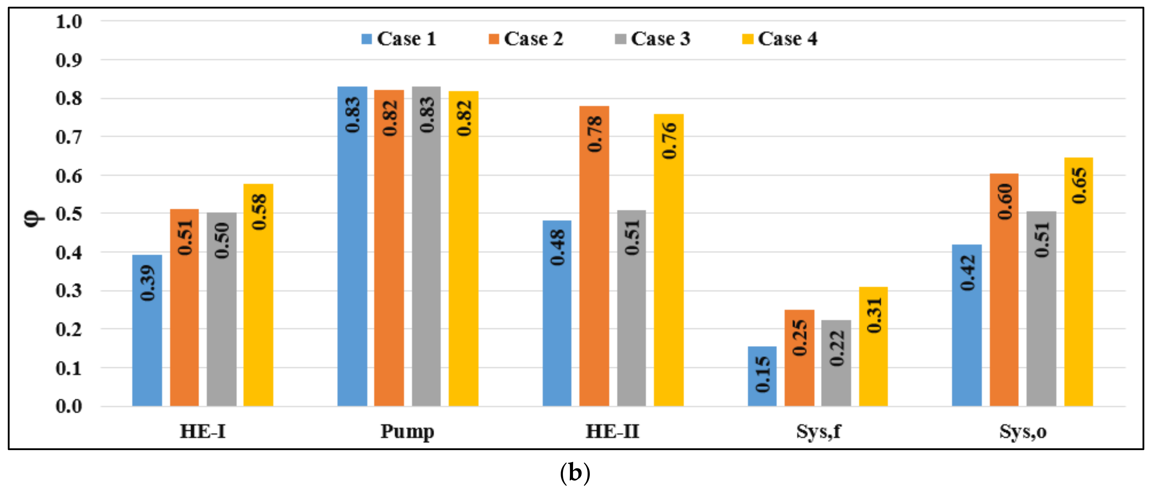
As presented in Figure 4b, the lowest exergy efficiency values were calculated in case one, followed by case three, case two, and case four, respectively, for the whole system ( φ s y s , f , φ s y s , o ) and for the HE-I ( φ H E I ). Therefore, it may be concluded that the heat potential of the WH source is used more effectively in case four, followed by case two, case three, and case one, respectively, to produce the useful energy for the DH network supply and the dwellings. However, the exergy efficiency of HE-II ( φ H E I I ) was determined to be as high as 0.78 in case two, rather than 0.76 in case four. This is because the exergy fuel rate of this component is 2.80 times more in case two than case four, while the exergy production rate is 2.87 times more in case two than case four. Meanwhile, although the exergy rate of the WH source (see Figure 3) changed from 220.90 kW (case four) to 4903 kW (case one), the exergy efficiency values belonging to the pump ( φ P u m p ) were found to be almost similar in all the created cases, varying between 0.82 and 0.83.
As shown in Figure 4a,b, the exergy destruction rates, due to the pump, were quite low (0.12 kW–1.27 kW) among other system components (21.65 kW–810 kW for HE-II and 65.26 kW–2413 kW for HE-I). In addition, the exergy efficiency values belonging to these components were higher (0.82–0.83) among other system components (0.48–0.78 for HE-II and 0.39–0.58 for HE-I). When two HEs were assessed together, higher exergy destruction rates (65.26 kW–2413 kW to 21.65 kW–810 kW) and lower exergy efficiencies (0.39–0.58 to 0.48–0.78) were observed for HE-I in all the cases. Therefore, it can be concluded that the priority for improvement should be given to HE-I, then HE-II, and finally the pump, based on the conventional exergy assessment. However, this analysis fails to identify the origin of the exergy destruction rates, namely, from the component itself (endogenous) or due to other components (exogenous), and can be (avoidable), or cannot be, (unavoidable) enhanced under the current technology status. In this regard, the advanced exergy performances of the employed components in each created case were assessed, and the obtained results are illustrated in Figure 5 and Figure 6, based on the endogenous/exogenous and avoidable/unavoidable splitting parts of exergy destruction rates, respectively.
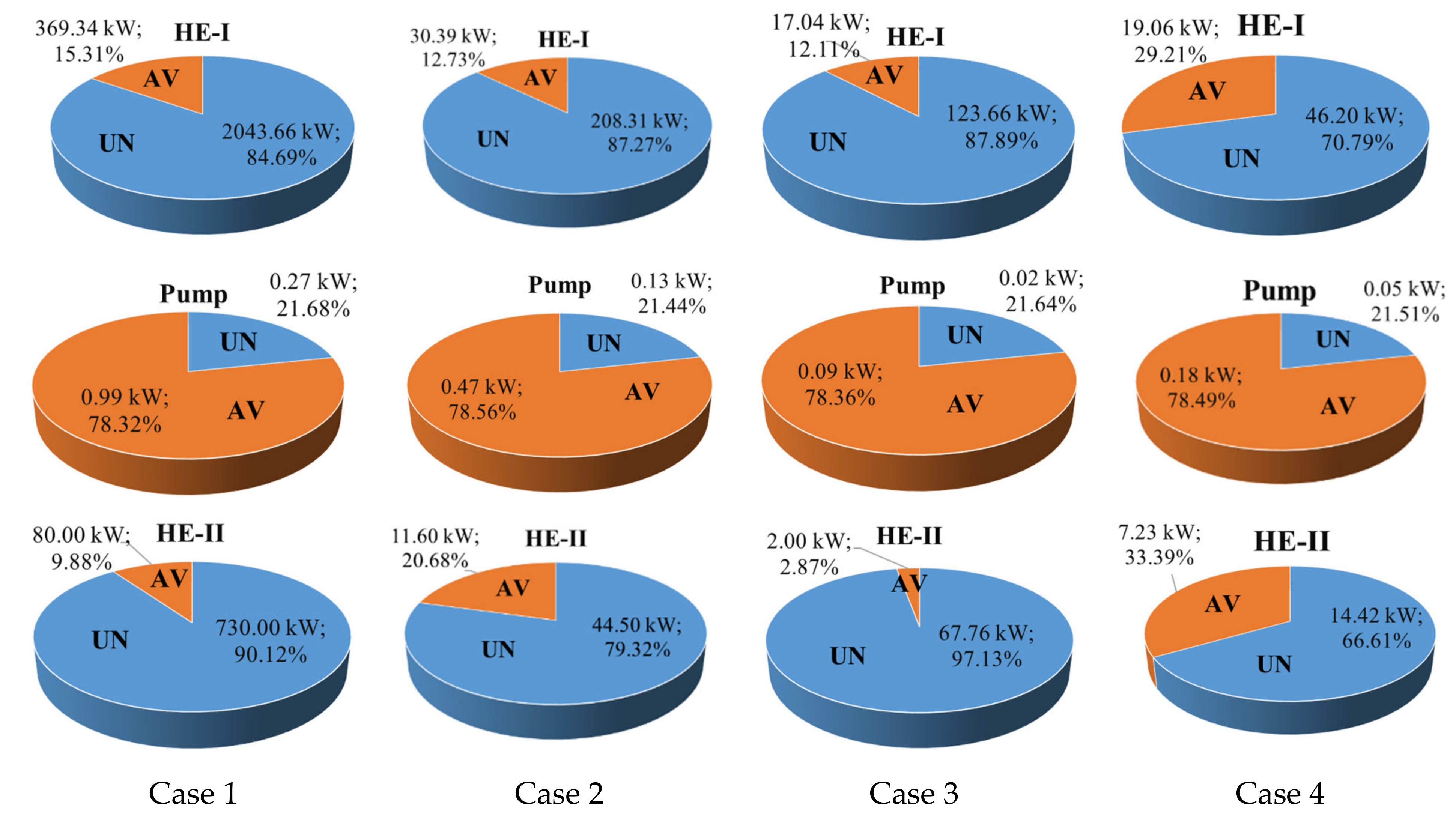
As observed in Figure 5, the exergy destruction rate, due to the pump, is mostly avoidable, ranging from 78.32% (case one) to 78.56% (case two). The simulated values for the avoidable exergy destruction rate of the remaining cases are 78.36% (case three) and 78.56% (case two). These obtained results show that the possible minimum exergy destruction rate can be realized between 0.02 kW in case three and 0.27 kW in case one under today’s technological status for the pump. On the other hand, as shown in the above figure, the exergy destruction rates that occurred in the HEs are mostly unavoidable, ranging between 70.79% (case four) and 87.89% (case three) for HE-I, and between 66.61% (case four) and 97.13% (case three) for HE-II. The simulated values for the unavoidable exergy destruction rate of the remaining cases are 84.69% (case one) and 87.27% (case two) for HE-I, and 90.12% (case one) and 79.32% (case two) for HE-II. These obtained results reveal that if the maximum possible operation condition is provided for the HEs considering the current technological status, most of the exergy destruction rate cannot be avoided (unavoidable), ranging between 46.20 kW in case four and 2043.66 kW in case one for HE-I, between 14.42 kW in case four and 730 kW in case one for HE-II. Therefore, it can be concluded that the priority for improvement should be given to the pump in all cases, based on the advanced exergy assessment considering the avoidable and unavoidable splitting parts of the exergy destruction rate. After this component, HE-I in cases one and three should be improved, similarly to HE-II in cases two and four.
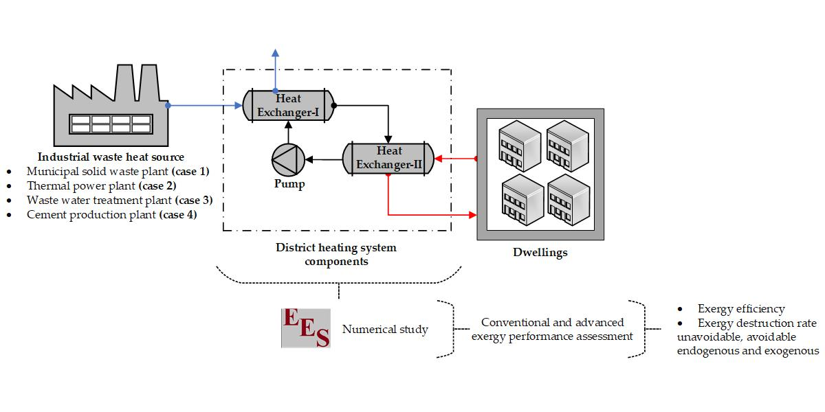
As shown in Figure 6, the exergy destruction rates that arose in the system components are mostly endogenous, which are as low as 69.80% (case four) for HE-II, and as high as 99.45% (case two) for the pump. These obtained results show that the interactions among the system components are not strong; in other words, the exergy destruction rates are mostly due to the component itself. On the other hand, if the remaining components operate under the hypothetical ideal condition (see Table 3), together with the studied component operating under the actual condition, the exergy destruction can be reduced to as low as 0.55% (case two) for the pump, and as high as 30.20% (case four) for HE-II. Therefore, it may be concluded that the origin of the exergy destruction rate is quite low, due to the remaining system components ranging between 0.002 kW and 313.93 kW, which shows the exogenous part of exergy destruction. As observed in the above figure, the endogenous part of the exergy destruction changes from 0.133 kW (case two for the pump) to 2099.07 kW (case one for HE-I).
The obtained results of conventional and advanced exergy analyses were also compared with the literature studies, based on the component level, considering the performance indicators, namely, the exergy efficiency and splitting parts of the exergy destruction rate (avoidable, unavoidable, endogenous, exogenous). Hepbasli and Keçebaş [9] assessed the performance of a geothermal DHS in Turkey, through conventional and advanced exergetic analysis methods, based on real operational data. The exergy efficiency for the six HEs and seven circulation pumps in the real Afyon geothermal DHS, were calculated from 0.45 to 0.84 and from 0.49 to 0.91, respectively. Meanwhile, the exergy destruction rates that arose in the system components were found to be mostly endogenous, ranging between 51.80% and 65.70% for HEs, and between 21.69% and 46.66% for the pumps. On the other hand, the exergy destruction rates, due to the HEs, were determined to be mostly avoidable, between 72.60% and 92.41%, whereas they were mostly unavoidable for the pumps between 53.34% and 75.49%. Yamankaradeniz [11] assessed the conventional and advanced exergy performances of a geothermal DHS located in Bursa, in Turkey, considering four HEs and four pumps located after the HEs. While the exergy efficiencies were determined from 79.68% to 97.05% for the HEs, they were calculated from 79.36% to 87.20% for the pumps. Meanwhile, the exergy destruction rates that occurred in the components were determined to be mostly avoidable, varying between 86.32% and 98.12%, and between 75.03% and 86.45%, respectively, for the HEs and pumps. Besides, the exergy destruction rates were determined to be mostly endogenous for the HEs two to four (between 65.25% and 79.89%), whereas they were mostly exogenous for HE 1 (63.65%) and for the employed pumps (between 95.61% and 97.50%). Liao et al. [22] conducted advanced exergy analysis for ORC-based layout, to recover the WH of flue gas. The thermodynamic performance of a proposed ORC–ORC system revealed that the exergy efficiencies of low-temperature HE, high-temperature HE, pump one and pump two, were 51.47%, 62.49%, 80.65% and 80.64%, respectively. Meanwhile, the splitting parts of the exergy destruction rates were simulated mostly endogenous for the considered components, varying between 91.24% for high-temperature HE and 100% for low-temperature HE. Besides, the exergy destruction rates occurring in the considered components were found to be mostly unavoidable for the HEs (89.75% for high-temperature HE and 100% for low-temperature HE), whereas they were mostly avoidable for the pumps, with a rate of 78.62%. Wang et al. [38] applied a conventional and advanced exergy assessment method to a cascade absorption heat transformer, for the recovery of low-grade waste heat. The simulated results of the proposed system showed that the exergy efficiencies of the HEs (lithium bromide and ammonia) and pumps (lithium bromide and ammonia) varied from 90.05% to 94.32%, and from 25.45% to 60.69%, respectively. Meanwhile, the exergy destruction rates occurring in the HEs were computed as mostly exogenous, which were 76.16% for lithium bromide HE and 78.65% for ammonia HE. On the other hand, the exergy destruction rates occurring in the pumps were calculated to be mostly endogenous, which ranged from 86.74% to 87.80% for lithium bromide pumps and from 89.01% to 89.57% for ammonia pumps. For the avoidable and unavoidable splitting parts, the dominant part was determined to be unavoidable for each system component, which was as low as 80.13% for ammonia–HE and as high as 82.46% for lithium bromide pump one. Oyekale et al. [43] applied advanced exergy analysis to a hybrid solar-biomass ORC plant having an organic fluid pump and HEs (condenser and evaporator). Based on the conventional exergy assessment, the exergy efficiencies were computed as almost 80% for the pump, almost 28% for the condenser, and 85% for the evaporator. Based on the advanced exergy analysis, the exergy destruction rates were found to be mostly endogenous (80% for the pump, 80.60% for the condenser, and 90.30% for the evaporator) and avoidable (80% for the pump, 77.50% for the condenser, and 88.10% for the evaporator). The comparison of the results of these literature studies with the presented study is summarized in Table 5.
As observed in Table 5, the exergy performance indicators (exergy efficiency in the conventional exergy assessment and splitting parts of the exergy destruction rate, unavoidable and endogenous, in the advanced exergy assessment) vary in very different ranges. The main reason for this is the choice of the dead state values, determination of endogenous and unavoidable conditions, and the type of fluid used. As a result of the selection of these parameters, the closest exergy efficiency values for HEs and pumps appeared in Ref. [9] and in Ref. [22], respectively. On the other hand, the closest values for the endogenous and unavoidable parts of exergy destruction were observed in Ref. [22], both for HEs and pumps.

4.3. Key Parameters and Their Effects on an Actual Implementation

In Turkey, the WH potential of the considered plants, based on the created cases, namely, municipal solid waste (case one), thermal power (case two), wastewater treatment (case three), and cement production (case four), is remarkably high. At the end of 2018, the total number of municipalities around the country was 1399, having an average amount of municipal solid waste per capita of 1.16 kg/day [27]. For the same year, 37.2% of the electricity need of Turkey was generated by coal-based thermal power plants, with a total number of 68 [44]. Meanwhile, the total number of wastewater treatment plants in Turkey reached 991 by the end of 2018, where approximately 4237 Mm3/year of wastewater was treated [30]. Finally, as of 2016, 71.4 million tons of production was realized by 70 cement production plants (52 integrated facilities and 18 grinding–packaging facilities) [45].
In this study, the functional exergy efficiency of the whole system (see Equation (8)) was recalculated when the WH potential of the municipal solid waste plant (case one was selected because it is more in number) was met with the DH system in the real world. In this regard, the key parameters were determined to be the ambient (dead state) temperature and the heat loss in the DH network for the selected sites, where soil temperature, the depth where the pipes are placed, and the geometric and thermal properties of the pipes become important. Therefore, as shown in Figure 7, four different provinces were selected, considering degree-day regions in Turkey and the situation with the highest population density [46,47]. Consequently, the İstanbul, İzmir, Ankara, and Kayseri provinces were determined to represent zones one, two, three, and four, respectively.
The long-term (1929–2020) average ambient temperature (Ta,ave) values measured in the seasonal normal of the selected provinces were considered for the winter months (October, December, January, February), using the weather forecast from the Turkish State Meteorological Service [48], and the obtained values are given in Table 6. In this table, the average soil temperature (Ts,ave) values below 100 cm from the surface are also given based on each month, which was determined by using the annual average Ts,ave values [49] and by assuming that these values are identical with the monthly variation in the Ta,ave for the considered sites.
The heat losses in the DH network, during operation for the considered sites, were evaluated based on the supply and return sides, by using Equations (14) and (15) given below, respectively [50].
Q ˙ l , s u p = U t o t · π · D o · L · T 3 T s , a v e
Q ˙ l , r e t = U t o t · π · D o · L · T 6 T s , a v e
where Q ˙ l , s u p p and Q ˙ l , r e t illustrate the heat loss in the DH network at the supply and return sides, respectively, during operation in kW. The U t o t is the total heat transfer coefficient of the pipeline in W/m2 · K. The Do and L are the outer diameter and length of the pipeline in m, respectively. While the U t o t values were found by Equation (16) given below, and Do was considered as 157.8 mm for a typical DH system arrangement, defined as model A in Ref. [51]. For the L, four different distances between the WH source and the dwellings were considered, using 5, 10, 15 and 20 km values.
U t o t = 1 D o D i · h i + D o · ln D t / D i 2 · k s t + D o · ln D o / D t 2 · k i n s
where the outer (Do), inner (Di), and intermittent (inner with pipe wall thickness) (Dt) diameters were taken into account as 157.8 mm, 88.9 mm, and 95.3 mm, respectively, for a typical DH system arrangement, defined as model A in Ref. [51]. Meanwhile, the thermal conductivities of steel ( k s t ) and insulation ( k i n s ) were considered as 16.27 W/m·K and 0.0265 W/m·K, respectively [51]. To calculate the convective heat transfer coefficient on the inner surface (hi), the equation steps given below were used [34].
R e i = ρ * v e l * D i μ
v e l = m ˙ ρ * A c
N u = 0.023 * R e i 0.8 * P r 0.4
h i = k w * N u D i
In the above-given equations (from (17) to (20)), the density ( ρ ), viscosity ( μ ), Prandtl number (Pr), and thermal conductivity (kw) properties of water were calculated using built-in thermophysical property functions by the written code. Following the calculation of 
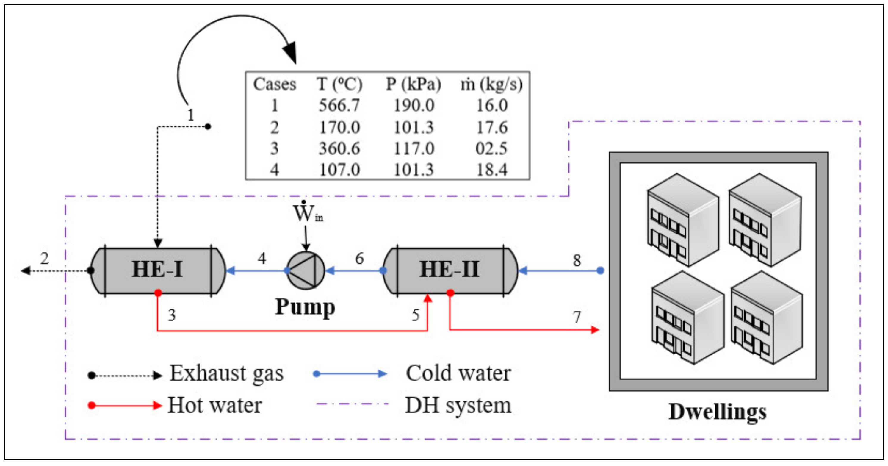
hi, the heat losses on the supply and return sides (see Equations (14) and (15)) were computed, which cause a temperature drop at states five and four (see Figure 2), respectively, considering the mass flow rates, the specific heats, and the inlet temperatures of the water (states three and six), given in Table 1. With these temperature drops, the simulated values for the functional exergy efficiency of the whole system are given in Table 7, based on case one.
As observed from Table 7, the highest functional exergy efficiencies were calculated for the shortest distances between the WH source and dwellings, based on each considered site. When all the zones are considered, the maximum functional exergy efficiencies were found between 0.1415 and 0.1782 for a 5 km distance. On the other hand, the minimum values were observed from 0.0519 to 0.0558 for a 20 km distance, considering all the zones. Note that, as given in Table 7, the average ambient temperature and the functional exergy efficiency are inversely proportional. When the shortest distance is considered (5 km) for all the zones, the highest functional exergy efficiency values were obtained in January, followed by February, December, and November, respectively. As shown in Table 6, these months are ordered from the coldest to the warmest. Therefore, it may be concluded that it is better to implement a WH source DH system with a possible shorter pipeline. Additionally, it is possible to operate with the highest functional exergy efficiency in colder ambient temperatures, although the heat loss would be higher. This is because this situation also affects the dead state temperature, which is highly significant on the functional exergy efficiency.

5. Conclusions

The main objectives of the present study were to investigate the conventional and advanced exergy performances of DHS options under various WH sources. A series of EES simulations were carried out to evaluate the effect of the created cases. Additionally, the key parameters and their effects on the actual implementation of the DHS were assessed through the analysis of 12 various cases (four different climate zones around the country, four winter months, and four different distances between the WH source and the dwellings for case one). While conducting these studies, the exergy efficiency and exergy destruction rate, with its splitting parts, were used as performance indicators. In the following, some concluding remarks are given:
  • The exergy destruction rates of the components, which also indicated the losses in work potentials, were simulated to be the highest for HE-I (between 65.26 kW and 2413 kW), followed by HE-II (from 21.65 kW to 810 kW), and the pump (between 0.12 kW and 1.27 kW), based on all the created cases;
  • The exergy destruction rates of the whole system that were obtained by the functional and overall exergy efficiency definitions, were determined to be the maximum in case one (4152 kW and 3224 kW, respectively), whereas they were the minimum in case four (153.6 kW and 87.1 kW, respectively);
  • The exergy efficiencies of the components, which also pointed out the priority, were found to be the highest for the pump, followed by HE-II and HE-I, considering all the created cases. For the functional and overall exergy efficiencies of the entire system, the lowest values were observed in case one, followed by cases three, two, and four;
  • The exergy destruction was found to be mostly avoidable for the pump, which was as high as 78.56% in case two. On the other hand, the splitting part of the exergy destruction was evaluated to be mostly unavoidable for the HEs, which varied from 70.79% in case four to 87.89% in case three for HE-I, and from 66.61% in case four to 97.13% in case three for HE-II;
  • The origin of exergy destruction was determined to be mostly endogenous for the pump and HEs (HE-I and HE-II), which was as high as 99.45% for the pump in case two and as low as 69.80% for HE-II in case four;
  • The highest functional exergy efficiencies were calculated for the shortest distances between the WH source and dwellings, based on each considered site, namely, İzmir, İstanbul, Ankara, and Kayseri. While the considerably low efficiency values were between 0.0519 and 0.0558 for the 20 km distance, considerably high efficiency values were determined from 0.1415 to 0.1782 for the 5 km distance;
  • The highest functional exergy efficiencies were computed for the coldest climates. Among all the selected sites and months, the maximum value was calculated in January in Kayseri, with an amount of 0.1782, where the minimum ambient average temperature was observed (−1.6 °C).

Author Contributions

Conceptualization, H.G.O., A.H. and A.A.; methodology, H.G.O., A.H. and A.A.; software, H.G.O.; validation, H.G.O.; formal analysis, H.G.O.; investigation, H.G.O., A.H. and A.A.; resources, H.G.O., A.H. and A.A.; data curation, H.G.O.; writing—original draft preparation, H.G.O.; writing—review and editing, H.G.O., A.H., A.A. and A.A.-M. All authors have read and agreed to the published version of the manuscript.

Funding

This research is part of the “HeatReFlex-Green and Flexible District Heating/Cooling” project (Available online: www.heatreflex.et.aau.dk (accessed on: 2 August 2021)) funded by the Danida Fellowship Centre and the Ministry of Foreign Affairs of Denmark to research in growth and transition countries under the grant no. 18-M06-AAU.

Institutional Review Board Statement

Ethical review and approval are not applicable for this study due to the reasons that the studies do not involving humans or animals.

Informed Consent Statement

Not applicable.

Data Availability Statement

Not applicable.

Acknowledgments

The authors acknowledge the support of the “HeatReFlex—Green and Flexible District Heating/Cooling” project (Available online: www.heatreflex.et.aau.dk (accessed on: 2 August 2021)) funded by the Danida Fellowship Centre and the Ministry of Foreign Affairs of Denmark to research in growth and transition countries under the grant no. 18-M06-AAU. They are also very grateful to the reviewers and editor for their valuable and constructive comments, which led to increasing the quality of the paper.

Conflicts of Interest

The authors declare no conflict of interest.

Abbreviations

DH(S)district heating (system)
EESengineering equation solver
HEheat exchanger
ORCorganic Rankine cycle
WHwaste heat
Nomenclature
E x ˙ exergy rate [kW]
Q ˙ heat transfer rate [kW]
W ˙ work consumption rate [kW]
m ˙ mass flow rate [kg/s]
Aarea [m2]
Ddiameter [m]
hspecific entalphy [kJ/kg]
k thermal   conductivity   [ W / m · K]
Llength [m]
Ppressure [kPa]
PrPrandtl number
ReReynolds number
s spesific   entrophy   [ kJ / kg · K]
Ttemperature [°C]
U heat   transfer   coefficient   [ W / m · K]
vspecific volume [m3/kg]
velvelocity [m/s]
Greek letters
sum operator
εeffectiveness
ηenergy efficiency
ѱspecific exergy [kJ/kg]
μ dynamic viscosity [kg/m·s]
ρ density [kg/m3]
Subscripts
0dead state
aambient
actactual
aveaverage
ccross sectional
ffunctional
iinner
ininput
insinsulation
isisentrophic
kcomponent “k”
lloss
maxmaximum
ooverall, outer
outoutput
retreturn
ssoil
ststeel
supsupply
syssystem
tthickness
tottotal
wwater
Superscripts
AVavoidable
ENendogenous
EXexogenous
UNunavaidable

References

  1. Mazhar, A.R.; Liu, S.; Shukla, A. A state of art review on the district heating systems. Renew. Sustain. Energy Rev. 2018, 96, 420–439. [Google Scholar] [CrossRef]
  2. Association, E.B. EU Handbooks-District Heating Markets; Bioenergy Europe: Brussels, Belgium, 2018. [Google Scholar]
  3. Millar, M.A.; Burnside, N.M.; Yu, Z. District heating challenges for the UK. Energies 2019, 12, 310. [Google Scholar] [CrossRef] [Green Version]
  4. International Renewable Energy Agency (IRENA) and Aalborg University, Integrating Low-Temperature Renewables in District Energy Systems: Guidelines for Policy Makers. Available online: https://www.irena.org/-/media/Files/IRENA/Agency/Publication/2021/March/IRENA_District_Energy_Systems_2021.pdf (accessed on 3 August 2021).
  5. Ljubenko, A.; Poredoš, A.; Morosuk, T.; Tsatsaronis, G. Performance analysis of a district heating system. Energies 2013, 6, 1298–1313. [Google Scholar] [CrossRef]
  6. Bühler, F.; Petrović, S.; Ommen, T.; Holm, F.M.; Pieper, H.; Elmegaard, B. Identification and evaluation of cases for excess heat utilisation using GIS. Energies 2018, 11, 762. [Google Scholar] [CrossRef] [Green Version]
  7. Zhang, L.; Wang, Y.; Feng, X. A framework for design and operation optimization for utilizing low-grade industrial waste heat in district heating and cooling. Energies 2021, 14, 2190. [Google Scholar] [CrossRef]
  8. Ji, C.; Qin, Z.; Dubey, S.; Choo, F.H.; Duan, F. Three-dimensional transient numerical study on latent heat thermal storage for waste heat recovery from a low temperature gas flow. Appl. Energy 2017, 205, 1–12. [Google Scholar] [CrossRef]
  9. Hepbasli, A.; Keçebaş, A. A comparative study on conventional and advanced exergetic analyses of geothermal district heating systems based on actual operational data. Energy Build. 2013, 61, 193–201. [Google Scholar] [CrossRef]
  10. Tan, M.; Keçebaş, A. Thermodynamic and economic evaluations of a geothermal district heating system using advanced exergy-based methods. Energy Convers. Manag. 2014, 77, 504–513. [Google Scholar] [CrossRef]
  11. Yamankaradeniz, N. Thermodynamic performance assessments of a district heating system with geothermal by using advanced exergy analysis. Renew. Energy 2016, 85, 965–972. [Google Scholar] [CrossRef]
  12. Yürüsoy, M.; Keçebaş, A. Advanced exergo-environmental analyses and assessments of a real district heating system with geothermal energy. Appl. Therm. Eng. 2017, 113, 449–459. [Google Scholar] [CrossRef]
  13. Sangi, R.; Jahangiri, P.; Thamm, A.; Müller, D. Dynamic exergy analysis—Modelica®-based tool development: A case study of CHP district heating in Bottrop, Germany. Therm. Sci. Eng. Prog. 2017, 4, 231–240. [Google Scholar] [CrossRef]
  14. Koroglu, T.; Sogut, O.S. Conventional and advanced exergy analyses of a marine steam power plant. Energy 2018, 163, 392–403. [Google Scholar] [CrossRef]
  15. Fellaou, S.; Bounahmidi, T. Analyzing thermodynamic improvement potential of a selected cement manufacturing process: Advanced exergy analysis. Energy 2018, 154, 190–200. [Google Scholar] [CrossRef]
  16. Mossi Idrissa, A.K.; Goni Boulama, K. Advanced exergy analysis of a combined Brayton/Brayton power cycle. Energy 2019, 166, 724–737. [Google Scholar] [CrossRef]
  17. Fitó, J.; Ramousse, J.; Hodencq, S.; Wurtz, F. Energy, exergy, economic and exergoeconomic (4E) multicriteria analysis of an industrial waste heat valorization system through district heating. Sustain. Energy Technol. Assess. 2020, 42, 13–15. [Google Scholar] [CrossRef]
  18. Fitó, J.; Hodencq, S.; Ramousse, J.; Wurtz, F.; Stutz, B.; Debray, F.; Vincent, B. Energy- and exergy-based optimal designs of a low-temperature industrial waste heat recovery system in district heating. Energy Convers. Manag. 2020, 211, 112753. [Google Scholar] [CrossRef]
  19. Pan, M.; Lu, F.; Zhu, Y.; Huang, G.; Yin, J.; Huang, F.; Chen, G.; Chen, Z. Thermodynamic, exergoeconomic and multi-objective optimization analysis of new ORC and heat pump system for waste heat recovery in waste-to-energy combined heat and power plant. Energy Convers. Manag. 2020, 222, 113200. [Google Scholar] [CrossRef]
  20. Allen, A.; Henze, G.; Baker, K.; Pavlak, G. Evaluation of low-exergy heating and cooling systems and topology optimization for deep energy savings at the urban district level. Energy Convers. Manag. 2020, 222, 113106. [Google Scholar] [CrossRef]
  21. Ambriz-Díaz, V.M.; Rubio-Maya, C.; Ruiz-Casanova, E.; Martínez-Patiño, J.; Pastor-Martínez, E. Advanced exergy and exergoeconomic analysis for a polygeneration plant operating in geothermal cascade. Energy Convers. Manag. 2020, 203, 112227. [Google Scholar] [CrossRef]
  22. Liao, G.; Jiaqiang, E.; Zhang, F.; Chen, J.; Leng, E. Advanced exergy analysis for Organic Rankine Cycle-based layout to recover waste heat of flue gas. Appl. Energy 2020, 266, 114891. [Google Scholar] [CrossRef]
  23. Chen, Y.; Hua, H.; Wang, J.; Lund, P.D. Thermodynamic performance analysis and modified thermo-ecological cost optimization of a hybrid district heating system considering energy levels. Energy 2021, 224, 120067. [Google Scholar] [CrossRef]
  24. Wang, Y.; Chen, Z.; Shen, Y.; Ma, Z.; Li, H.; Liu, X.; Zhu, Z.; Qi, J.; Cui, P.; Wang, L.; et al. Advanced exergy and exergoeconomic analysis of an integrated system combining CO2 capture-storage and waste heat utilization processes. Energy 2021, 219, 119600. [Google Scholar] [CrossRef]
  25. Caglayan, H.; Caliskan, H. Advanced exergy analyses and optimization of a cogeneration system for ceramic industry by considering endogenous, exogenous, avoidable and unavoidable exergies under different environmental conditions. Renew. Sustain. Energy Rev. 2021, 140, 110730. [Google Scholar] [CrossRef]
  26. Marchionni, M.; Bianchi, G.; Tsamos, K.M.; Tassou, S.A. Techno-economic comparison of different cycle architectures for high temperature waste heat to power conversion systems using CO2 in supercritical phase. Energy Procedia 2017, 123, 305–312. [Google Scholar] [CrossRef]
  27. Tozlu, A.; Abusoglu, A.; Ozahi, E.; Anvari-Moghaddam, A. Municipal solid waste-based district heating and electricity production: A case study. J. Clean. Prod. 2021, 297, 126495. [Google Scholar] [CrossRef]
  28. Yildiran, R.; Atas, S.; Researcher, S.; Kahraman, M.; Researcher, S. Design and Performance Analysis of a District Heating System. J.Therm. Eng. 2016, 2, 940–954. [Google Scholar]
  29. Erdem, H.H.; Dagdas, A.; Sevilgen, S.H.; Cetin, B.; Akkaya, A.V.; Sahin, B.; Teke, I.; Gungor, C.; Atas, S. Thermodynamic analysis of an existing coal-fired power plant for district heating/cooling application. Appl. Therm. Eng. 2010, 30, 181–187. [Google Scholar] [CrossRef]
  30. Abusoglu, A.; Tozlu, A.; Anvari-Moghaddam, A. District heating and electricity production based on biogas produced from municipal WWTPs in Turkey: A comprehensive case study. Energy 2021, 223, 119904. [Google Scholar] [CrossRef]
  31. Atmaca, A.; Yumrutaş, R. Thermodynamic and exergoeconomic analysis of a cement plant: Part II—Application. Energy Convers. Manag. 2014, 79, 799–808. [Google Scholar] [CrossRef]
  32. Fang, H.; Xia, J.; Jiang, Y. Key issues and solutions in a district heating system using low-grade industrial waste heat. Energy 2015, 86, 589–602. [Google Scholar] [CrossRef]
  33. Fchart Engineering Equation Solver. 2015. Available online: http://www.fchart.com/ees (accessed on 2 August 2021).
  34. Cengel, Y.A.; Cimbala, J.M.; Turner, R.H. Fundamentals of Thermal-Fluid Sciences, 5th ed.; McGraw-Hill Education: New York, NY, USA, 2016. [Google Scholar]
  35. Ghaebi, H.; Ahmadi, S. Energy and exergy evaluation of an innovative hybrid system coupled with HRSG and HDH desalination units. J. Clean. Prod. 2020, 252, 119821. [Google Scholar] [CrossRef]
  36. Arabkoohsar, A.; Alsagri, A.S. Thermodynamic analysis of ultralow-temperature district heating system with shared power heat pumps and triple-pipes. Energy 2020, 194, 116918. [Google Scholar] [CrossRef]
  37. Riahi, S.; Jovet, Y.; Saman, W.Y.; Belusko, M.; Bruno, F. Sensible and latent heat energy storage systems for concentrated solar power plants, exergy efficiency comparison. Sol. Energy 2019, 180, 104–115. [Google Scholar] [CrossRef]
  38. Wang, Y.; Liu, Y.; Liu, X.; Zhang, W.; Cui, P.; Yu, M.; Liu, Z.; Zhu, Z.; Yang, S. Advanced exergy and exergoeconomic analyses of a cascade absorption heat transformer for the recovery of low grade waste heat. Energy Convers. Manag. 2020, 205, 112392. [Google Scholar] [CrossRef]
  39. Mohammadi, Z.; Fallah, M.; Mahmoudi, S.M.S. Advanced exergy analysis of recompression supercritical CO2 cycle. Energy 2019, 178, 631–643. [Google Scholar] [CrossRef]
  40. Araz, M.; Hepbasli, A.; Biyik, E.; Shahrestani, M.; Yao, R.; Essah, E.; Shao, L.; Oliveira, A.C.; Ekren, O.; Günerhan, H. Performance evaluation of a building integrated photovoltaic (BIPV) system combined with a wastewater source heat pump (WWSHP) system. Energy Procedia 2017, 140, 434–446. [Google Scholar] [CrossRef]
  41. Zhang, Y.; Yao, E.; Wang, T. Comparative analysis of compressed carbon dioxide energy storage system and compressed air energy storage system under low-temperature conditions based on conventional and advanced exergy methods. J. Energy Storage 2021, 35, 102274. [Google Scholar] [CrossRef]
  42. Aghaziarati, Z.; Aghdam, A.H. Thermoeconomic analysis of a novel combined cooling, heating and power system based on solar organic Rankine cycle and cascade refrigeration cycle. Renew. Energy 2021, 164, 1267–1283. [Google Scholar] [CrossRef]
  43. Oyekale, J.; Petrollese, M.; Cau, G. Modified auxiliary exergy costing in advanced exergoeconomic analysis applied to a hybrid solar-biomass organic Rankine cycle plant. Appl. Energy 2020, 268, 114888. [Google Scholar] [CrossRef]
  44. Republic of Turkey Ministry of Energy and Natural Resources, Info Bank Energy-Electricity. Available online: https://enerji.gov.tr/bilgi-merkezi-enerji-elektrik-en (accessed on 9 July 2021).
  45. Turkey İsbank, Department of Economic Research-Cement Sector in Turkey in 2016. Available online: https://ekonomi.isbank.com.tr/ContentManagement/Documents/sr201604_cimentosektoru.pdf (accessed on 9 July 2021).
  46. Statistical Information about the Population of Turkey. Available online: https://www.nufusu.com/ (accessed on 9 July 2021).
  47. Turkish Standard, T.S. 825 Thermal insulation requirements for buildings. Turk. Stand Inst. Ank. 2008, 825, 80. [Google Scholar]
  48. Turkish State Meteorological Service, Extreme Maximum, Minimum and Average Temperatures Measured in Long Period for Cities and Holiday Resorts. Available online: https://www.mgm.gov.tr/eng/forecast-cities.aspx?m=IZMIR (accessed on 9 July 2021).
  49. Turkish State Meteorological Service, Turkey 100 cm Soil Temperatures. Available online: http://www1.mgm.gov.tr/FILES/resmi-istatistikler/Turkiye-100cm-Toprak-Sicakliklari.pdf (accessed on 9 July 2021).
  50. District Heating Pipe Catalogue. Available online: http://www.polytherm.ie/v4/0940aa0c-5421-4a9b-840d-c9a2ae5d95bb/uploads/Premant%20Technical%20Catalogue.pdf (accessed on 9 July 2021).
  51. Xu, Q.; Wang, K.; Zou, Z.; Zhong, L.; Akkurt, N.; Feng, J.; Xiong, Y.; Han, J.; Wang, J.; Du, Y. A new type of two-supply, one-return, triple pipe-structured heat loss model based on a low temperature district heating system. Energy 2021, 218, 119569. [Google Scholar] [CrossRef]
Figure 1. Topology of the studied system.
Energies 14 04766 g001
Figure 2. Flowsheet of the exergy assessment method.
Energies 14 04766 g002
Figure 3. Grassmann (exergy flow) diagram of the created cases, (a) case one, (b) case two, (c) case three and (d) case four.
Energies 14 04766 g003aEnergies 14 04766 g003b
Figure 4. Conventional exergy assessment results based on (a) exergy destruction rate and (b) exergy efficiency.
Energies 14 04766 g004aEnergies 14 04766 g004b
Figure 5. Advanced exergy assessment results respect to avoidable and unavoidable parts.
Energies 14 04766 g005
Figure 6. Advanced exergy assessment results with respect to endogenous and exogenous parts.
Energies 14 04766 g006
Figure 7. Provinces in Turkey by degree-day regions.
Energies 14 04766 g007
Table 1. Thermo-physical properties of the state points given in Figure 1 based on created cases.
StateFluidT (°C)P (kPa) m ˙ (kg/s)
Case 1Case 2Case 3Case 4Case 1Case 2Case 3Case 4Case 1Case 2Case 3Case 4
0′Water20.0100.0-
0″Air
1Air566.7170.0360.6107.0190.0120.0117.0101.316.017.602.518.4
2Air71.050.071.060.0190.0120.0117.0101.316.017.602.518.4
3Water130.074.0130.070.0600.0420.0600.0420.029.023.002.608.9
4Water70.054.070.050.0600.0420.0600.0420.029.023.002.608.9
5Water130.074.0130.070.0600.0420.0600.0420.029.023.002.608.9
6Water70.054.070.050.0400.0306.0400.0306.029.023.002.608.9
7Water68.065.568.065.0400.0306.0400.0306.085.925.008.207.6
8Water50.049.050.045.0400.0180.0400.0180.085.925.008.207.6
Table 2. Specific entropy, enthalpy and exergy values of the state points given in Figure 1 based on created cases.
StateFluids (kJ/kg·K)h (kJ/kg)ѱ (kJ/kg)
Case 1Case 2Case 3Case 4Case 1Case 2Case 3Case 4Case 1Case 2Case 3Case4
0′Water0.296584.010
0″Air6.845293.30
1Air7.75507.21107.58907.1040866.3445.1643.0381.1306.444.6131.612.0
2Air6.82206.98106.96206.9710344.6323.5344.7333.658.016.817.203.6
3Water1.63401.00301.63400.9549546.6310.1546.6293.470.418.970.416.4
4Water0.95480.75510.95480.7036293.5226.4293.5209.716.508.016.506.3
5Water1.63401.00301.63400.9549546.6310.1546.6293.470.418.970.416.4
6Water0.95490.75510.95490.7037293.4226.3293.4209.616.307.916.306.2
7Water0.93040.89970.93040.8935285.0274.4285.0272.315.113.615.113.3
8Water0.70360.69080.70360.6385209.7205.3209.7188.606.305.706.304.3
Table 3. Actual, unavoidable, and ideal conditions of components in the WH source DH system based on created cases.
ComponentkParameterActualUnavoidableIdeal
Case 1Case 2Case 3Case 4Case 1Case 2Case 3Case 4Case 1Case 2Case 3Case 4
HE-Iε0.880.900.900.850.95 [21,22,42]1 [21,22,42]
Pumpηis 0.80 [22,42,43]
HE-IIε0.880.900.930.85
Table 4. Results of the validation of the develop model for case one.
Performance IndicatorRef. [27]Present WorkRelative Error
E x ˙ D , H E I 2412 kW2412 kW0%
E x ˙ D , P u m p 0.3 kW0.3 kW0%
E x ˙ D , H E I I 810 kW810 kW0%
E x ˙ D , s y s , f 4914.2 kW4151 kW15.5%
φ H E I 39.3%39.3%0%
φ P u m p 95.2%95.2%0%
φ H E I I 48.3%48.3%0%
φ s y s , f 09.4%15.4%63.8%
Table 5. Comparison of the exergy performance indicators considering the conducted literature studies.
IndicatorRefs.Presented Study
Ref. [9]Ref. [11]Ref. [22]Ref. [38]Ref. [43]
φ H E 0.45–0.840.80–0.970.51–0.620.90–0.940.27–0.850.39–0.78
φ P u m p 0.49–0.910.79–0.870.80–0.810.25–0.610.79–0.800.82–0.83
E ˙ x D , H E E N / E x ˙ D , H E 0.52–0.660.36–0.800.91–1.000.21–0.230.81–0.900.69–0.92
E ˙ x D , H E U N / E x ˙ D , H E 0.08–0.270.02–0.140.90–1.000.79–0.810.11–0.230.66–0.98
E ˙ x D , P u m p E N / E x ˙ D , P u m p   0.22–0.472.50–4.410.96–0.980.86–0.880.79–0.800.97–1.00
E ˙ x D , P u m p U N / E x ˙ D , P u m p 0.53–0.750.14–0.250.21–0.220.81–0.830.79–0.800.20–0.21
Table 6. Average ambient and soil (buried 100 cm) temperature values of the considered sites.
Effecting ParametersConsidered MonthsSelected ProvincesZones
NovemberDecemberJanuaryFebruary
Ta,ave (°C)14.210.58.89.6İzmirI
13.49.26.97.9İstanbulII
7.22.50.21.7AnkaraIII
5.50.7−1.60.2KayseriIV
Ts,ave (°C)15.411.49.610.4İzmirI
13.49.26.97.9İstanbulII
8.83.10.22.1AnkaraIII
6.70.9−2.00.2KayseriIV
Table 7. Obtained functional exergy efficiency results of the whole system based on case one.
Distance Considered MonthsSelected ProvincesZones
NovemberDecemberJanuaryFebruary
5 km0.14150.15090.15490.1531İzmirI
10 km0.11080.11700.11970.1187
15 km0.08170.08510.08650.0858
20 km0.05430.05480.05490.0548
5 km0.14320.15380.15930.1570İstanbulII
10 km0.11170.11890.12250.1207
15 km0.08160.08550.08730.0866
20 km0.05340.05410.05410.0541
5 km0.15890.16980.17450.1715AnkaraIII
10 km0.12290.12920.13190.1304
15 km0.08840.09080.09160.0911
20 km0.05580.05420.05290.0538
5 km0.16310.17360.17820.1745KayseriIV
10 km0.12510.13170.13430.1319
15 km0.08930.09150.09200.0916
20 km0.05530.05330.05190.0529
Publisher’s Note: MDPI stays neutral with regard to jurisdictional claims in published maps and institutional affiliations.

