
Modelling of Solar Irradiance Incident on Building Envelopes in Polish Climatic Conditions: The Impact on Energy Performance Indicators of Residential Buildings


Abstract
:1. Introduction
2. Literature Review
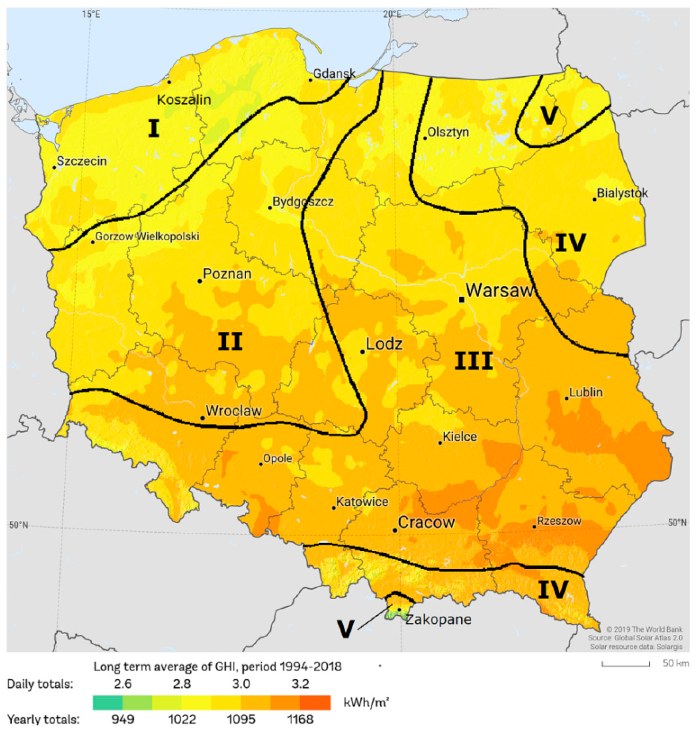
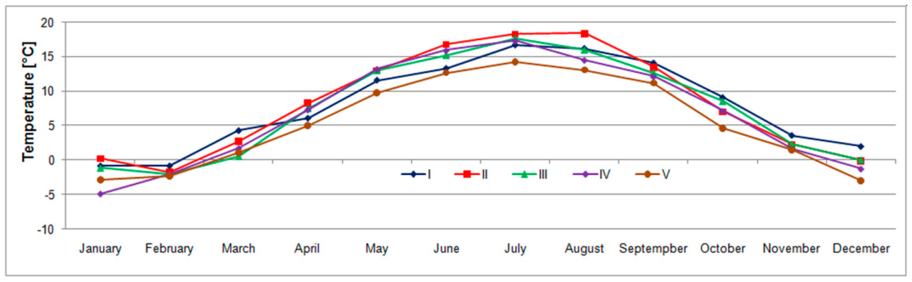
3. Polish Typical Meteorological Years
4. Modelling of Solar Irradiance on Sloped Surfaces
4.1. Introduction
teq = 5.2 + 9.0·cos[(nday − 43)·0.0357·180/π] if 20 ≤ nday < 136,
teq = 1.4 − 5.0·cos[(nday − 135)·0.0449·180/π] if 136 ≤ nday < 241,
teq = −6.3 − 10.0·cos[(nday − 306)·0.036·180/π] if 241 ≤ nday < 336,
teq = 0.45·(nday − 359) if nday ≥ 336,
cos(δ)·cos(φw)·cos(β)·cos(ω) + cos(δ)·sin(φw)·sin(β)·cos(γ)·cos(ω) +
cos(δ)·sin(β)·sin(γ)·sin(ω)].
4.2. Global Irradiance on a Sloped Surface
4.3. Transposition Models
4.3.1. TMY
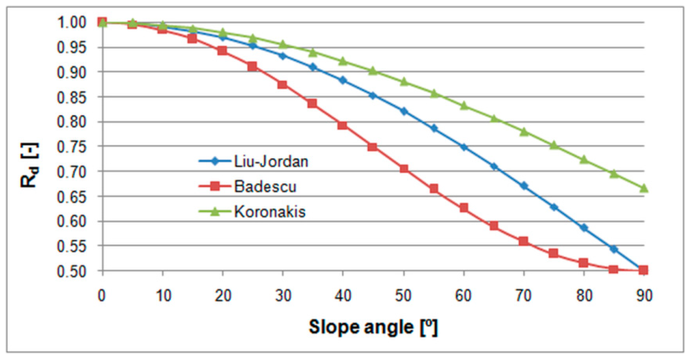
4.3.2. Liu-Jordan
4.3.3. Badescu
4.3.4. Koronakis
4.3.5. Circumsolar
4.3.6. Bugler
4.3.7. Klucher
4.3.8. Hay
4.3.9. Willmott
4.3.10. Ma and Iqbal
4.3.11. Skartveit and Olseth
4.3.12. Reindl
4.3.13. Gueymard
4.3.14. Muneer
4.3.15. Perez
4.3.16. EN ISO 52010
5. Materials and Methods
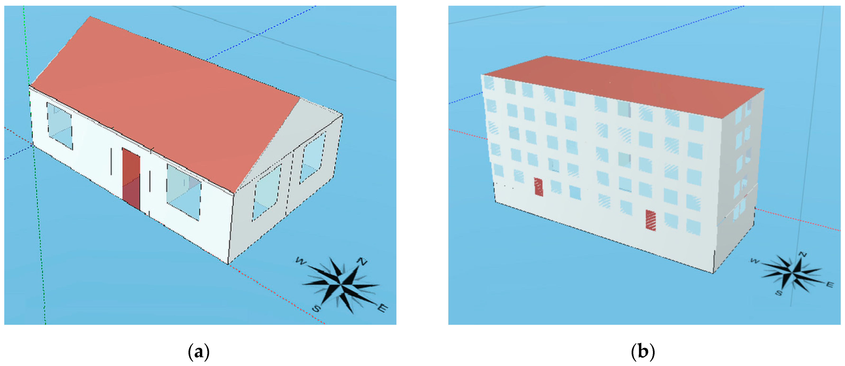
5.1. Test Buildings
5.2. Calculation of Solar Gains
5.3. Energy Performance Indicators
- The value of the annual demand for nonrenewable primary energy EP (kWh/m2) is lower or equal to the maximum value specified in the regulations (Table 6).
- The partitions and technical equipment of a building meet at least the thermal insulation requirements specified in Annex 2 of this Regulation (Table 7).
6. Results and Discussion
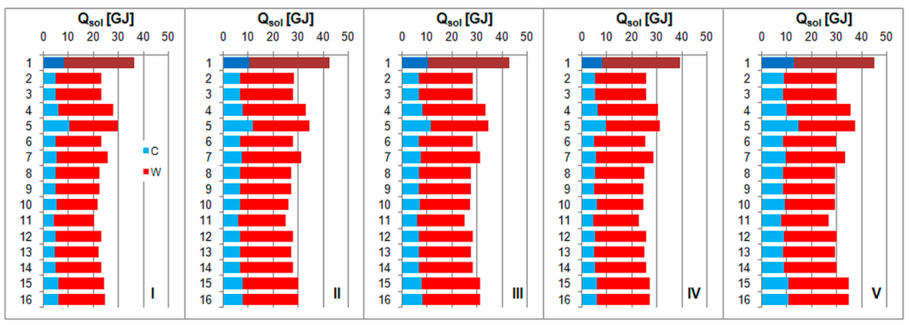
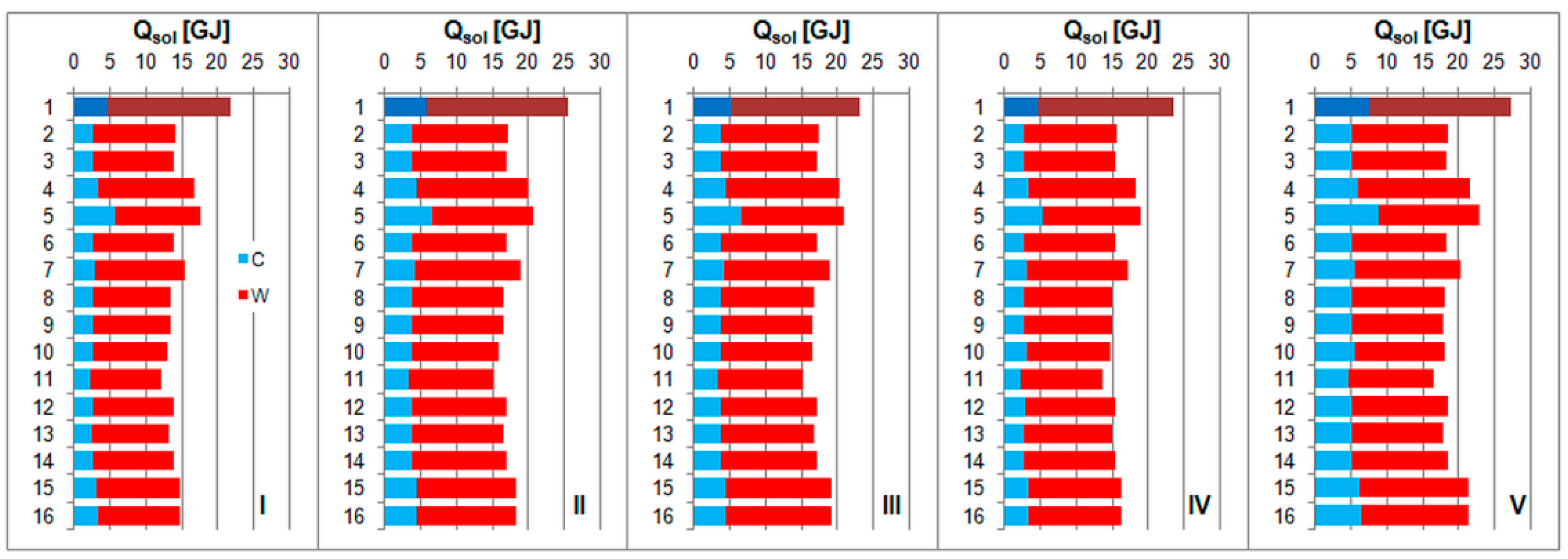
6.1. Solar Gains in the Single Family Building
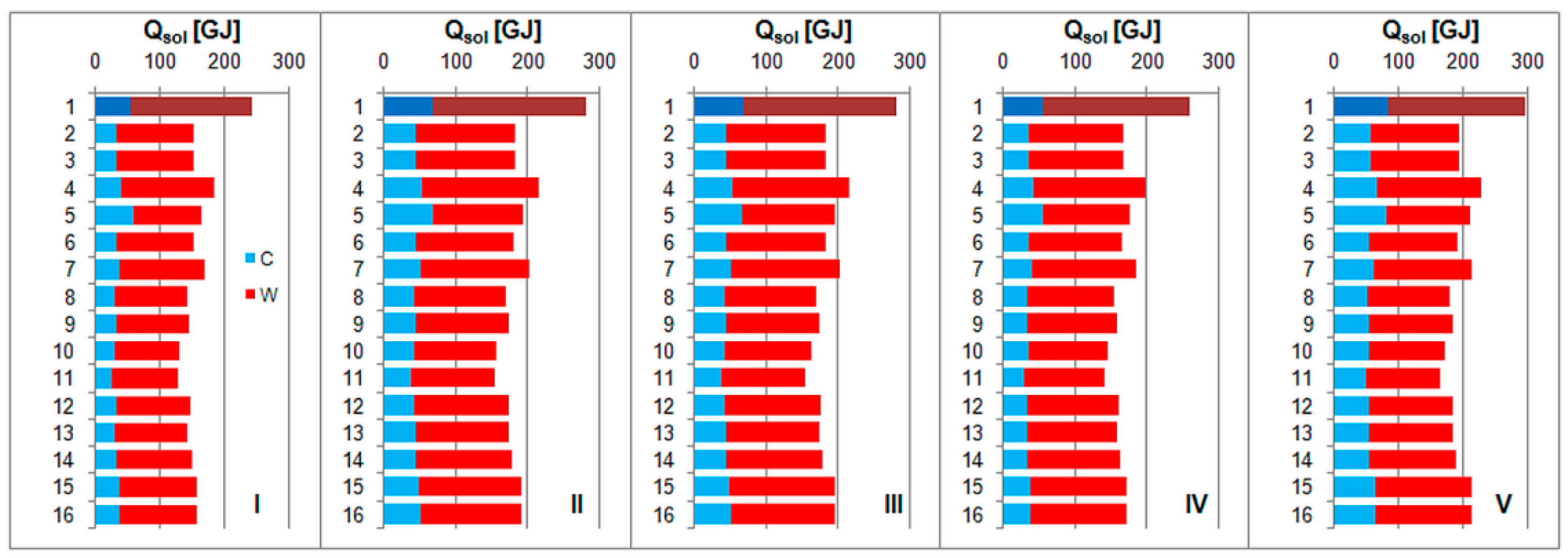
6.2. Solar Gains in the Multifamily Building
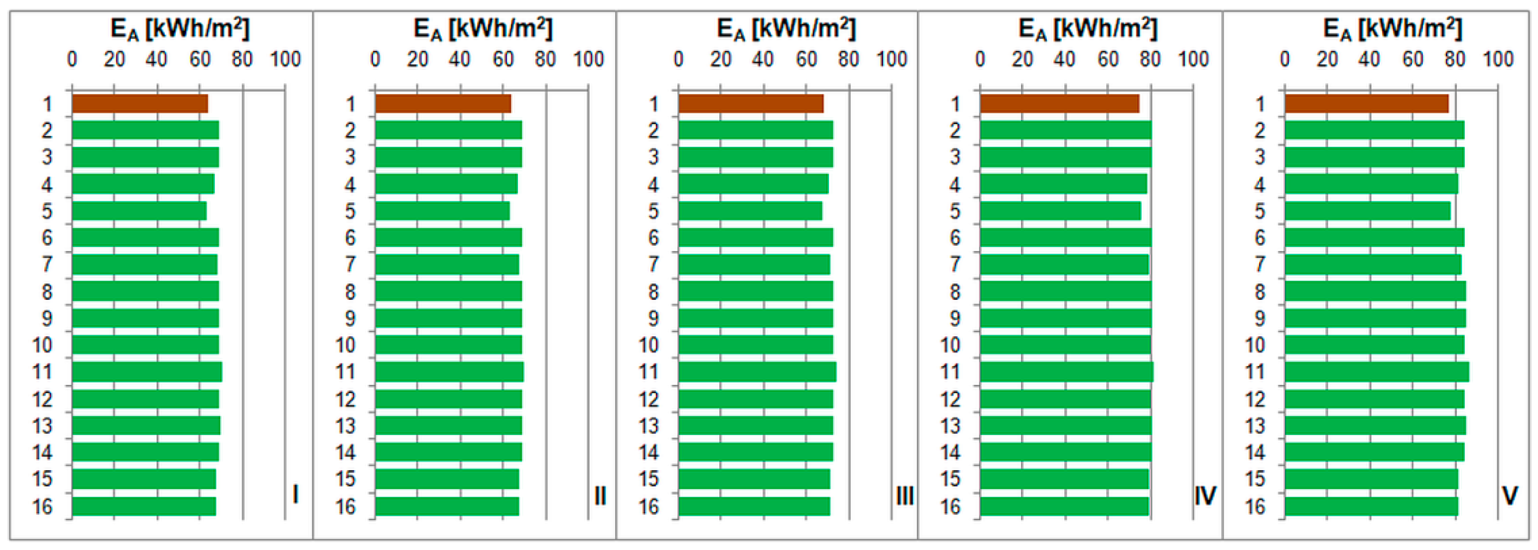
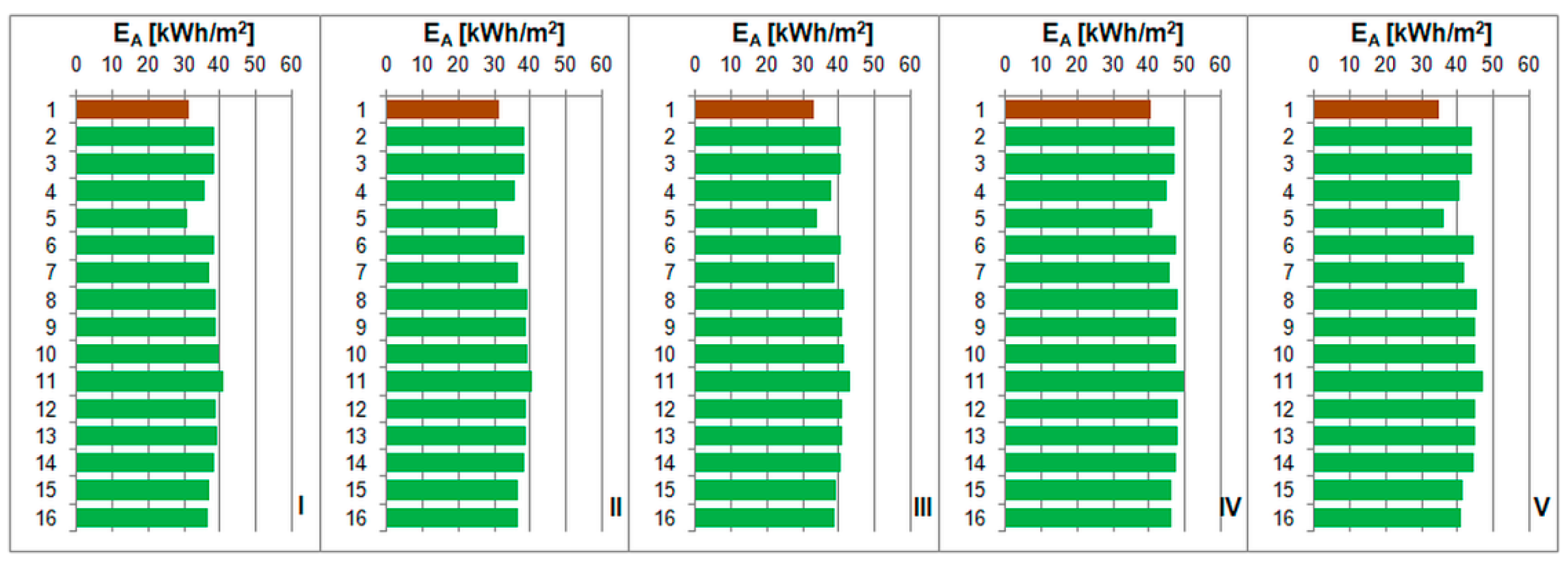
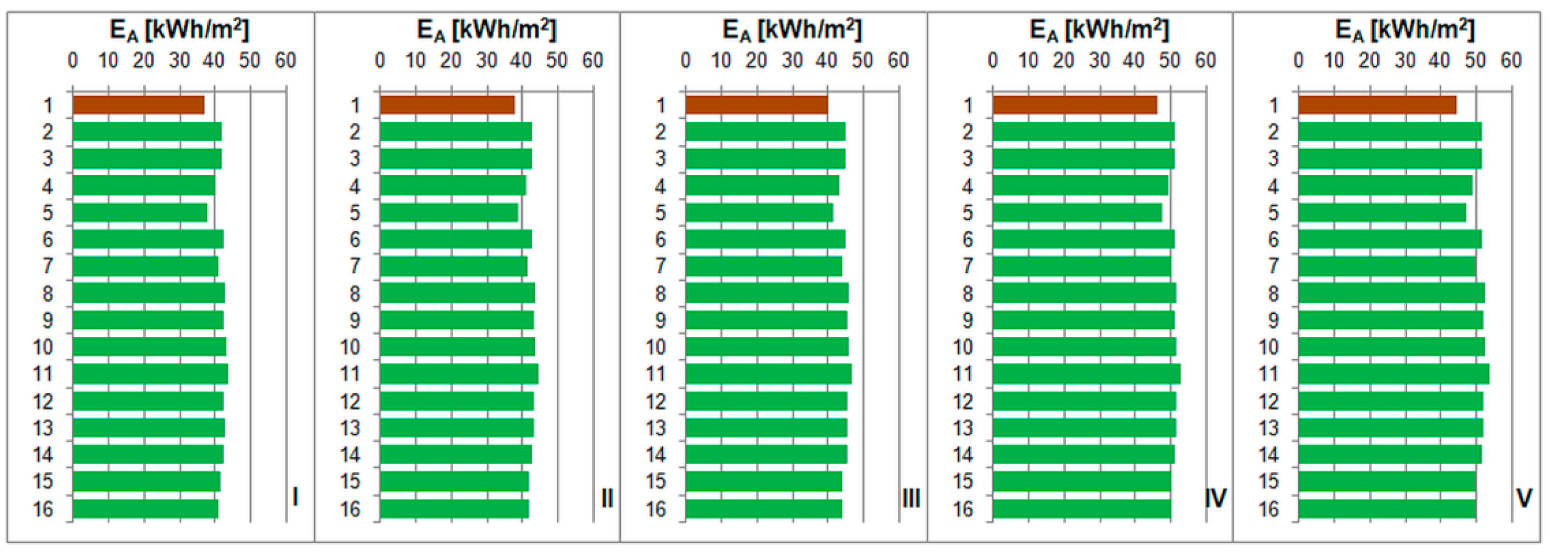
6.3. Annual Heating Energy Demand
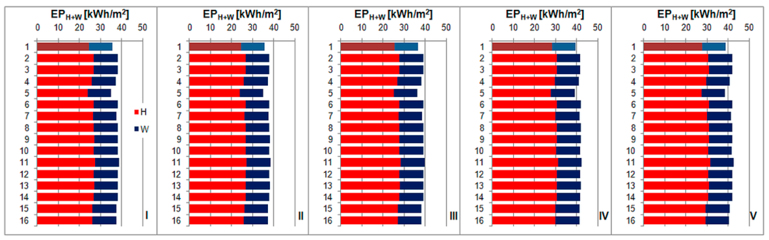
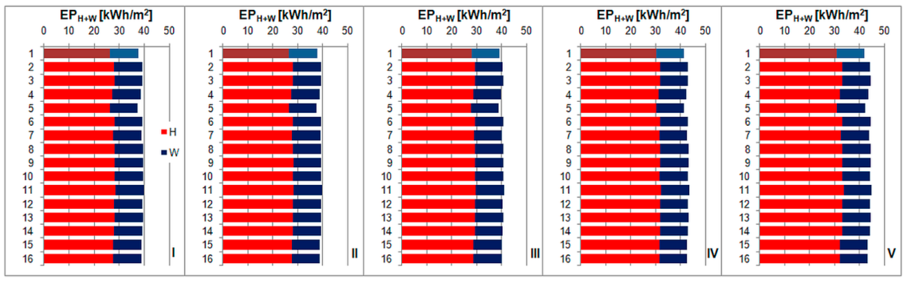
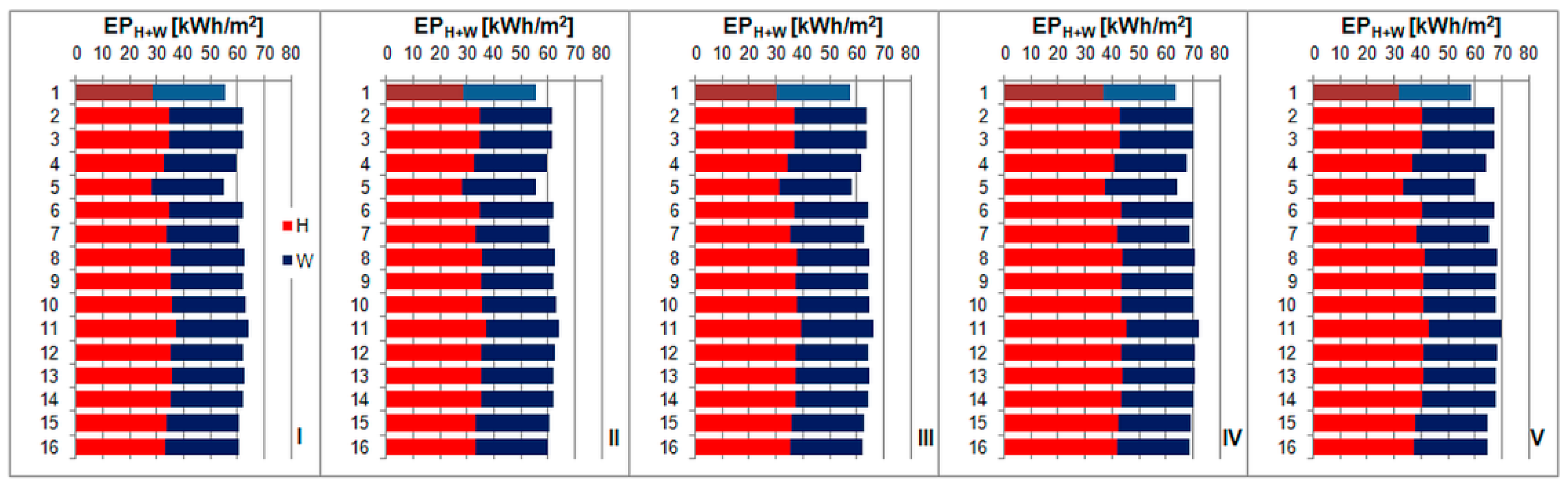
6.4. Energy Performance Indicators
7. Conclusions
Supplementary Materials
Funding
Institutional Review Board Statement
Informed Consent Statement
Data Availability Statement
Conflicts of Interest
Nomenclature
| Ac | —projected area of an envelope element, m2 |
| Asol | —effective collecting area of an envelope element, m2 |
| Af | —total conditioned (heated and/or cooled) floor area, m2 |
| Af,c | —total cooled floor area, m2 |
| Ac | —projected area of an envelope element, m2 |
| Asol | —effective collecting area of an envelope element, m2 |
| B | —Earth orbit deviation, ° |
| Cm | —internal thermal capacity of the considered building (or zone), J/K |
| EA | —annual heating energy demand per unit floor area of a building, kWh/m2 |
| EPH+W | —partial maximum value of the EP index for heating, ventilation and domestic hot water, kWh/m2 |
| EP | —index of the annual demand for nonrenewable primary energy, kWh/m2 |
| EU | —usable energy indicator, kWh/m2 |
| FF | —frame and divider area fraction of the glazed element |
| Fsky | —view factor between the element and the sky |
| Fsh,ob | —shading reduction factor for external obstacles |
| Fsh,gl | —shading reduction factor for movable shading provisions |
| F1 | —circumsolar brightness coefficient |
| F2 | —horizontal brightness coefficient |
| Gsol,c | —solar constant, 1370 W/m2 |
| H | —solar irradiation, kWh/m2 |
| Htr | —heat transfer coefficient by transmission, W/K |
| Hve | —heat transfer coefficient by ventilation, W/K |
| Ib,h | —direct (beam) solar irradiance on a horizontal surface, W/m2 |
| Ib,s | —direct (beam) solar irradiance on a sloped surface, W/m2 |
| Id,h | —diffuse solar irradiance on a horizontal surface, W/m2 |
| Id,s | —diffuse solar irradiance on a sloped surface, W/m2 |
| Iext | —extra-terrestrial irradiance, W/m2 |
| Iext,h | —extra-terrestrial irradiance on a horizontal surface, W/m2 |
| Ig,h | —global solar irradiance on a horizontal surface, W/m2 |
| Ig,s | —global solar irradiance on a sloped surface, W/m2 |
| Ir,s | —solar irradiance due to ground reflection on a sloped surface, W/m2 |
| Itot | —calculated total solar irradiance, W/m2 |
| Rb | —beam (direct) transposition factor |
| Qsol | —solar heat gain, J |
| Rd | —diffuse transposition factor |
| Rr | —reflected transposition factor |
| Rse | —external surface heat resistance of an element, m2·K/W |
| Tshift | —time shift, h |
| TZ | —time zone, h |
| U | —thermal transmittance, W/(m2·K) |
| Uc | — thermal transmittance of an envelope element of the area Ac, W/(m2·K) |
| f | —brightness coefficient (Perez model) |
| ggl | —monthly mean effective total solar energy transmittance |
| i | —month number |
| hr,e | —external radiative heat transfer coefficient, W/(m2·K) |
| kH | —anisotropy index (Hay model) |
| kR | —modulating factor (Reindl model) |
| kT | —clearness index of the atmosphere |
| m | —air mass |
| nday | —day of the year |
| nhour | —actual (clock) hour for the location (counting number of the hour in the day) |
| teq | —equation of time, min |
| ts | —solar time, h |
| ti | —internal air temperature, °C |
| Δ | —sky brightness parameter |
| ΔEPC | —partial value of the EP index for cooling, kWh/m2 |
| ΔEPL | —partial value of the EP index for lighting, kWh/m2 |
| Δθsky | — average difference between the external air temperature and the apparent sky temperature, K |
| Δτm | —length of the m-th month, s |
| Φr | —heat flow due to thermal radiation to the sky, W |
| Φsol | —heat flow by solar gains through a building element, W |
| αop | —absorption coefficient for solar radiation of the opaque element |
| αsol | —solar altitude angle, ° |
| β | —slope angle of inclined surface, ° |
| γ | —azimuth angle, ° |
| δ | —solar declination, ° |
| ε | —clearness parameter (Perez model) |
| θ | —angle of incidence of beam irradiance, ° |
| θz | —zenith angle, ° |
| λw | —longitude of a weather station, ° |
| ρ | —solar reflectivity of the ground and building’s surroundings |
| φw | —latitude of a weather station, ° |
| ω | —solar hour angle, ° |
References
- Energy Consumption in Households in 2018; Central Statistical Office: Warsaw, Poland, 2019. Available online: https://stat.gov.pl/en/topics/environment-energy/energy/energy-consumption-in-households-in-2018,2,5.html (accessed on 14 April 2021).
- Kozik, R.; Karasińska-Jaśkowiec, I. Green public procurement-legal base and instruments supporting sustainable development in the construction industry in Poland. E3S Web Conf. 2016, 10, 00044. [Google Scholar] [CrossRef] [Green Version]
- Ramczyk, M. Legal bases and economic conditions of applying renewable energy resources in construction industry. MATEC Web Conf. 2018, 174, 04004. [Google Scholar] [CrossRef]
- European Parliament and Council. Directive 2010/31/EU of the European Parliament and of the Council of 19 May 2010 on the energy performance of buildings (recast). Off. J. Eur. Union 2010, 13–35. Available online: http://eur-lex.europa.eu/LexUriServ/LexUriServ.do?uri=OJ:L:2010:153:0013:0035:EN:PDF (accessed on 14 April 2021).
- Gonzalez Caceres, A.; Diaz, M. Usability of the EPC tools for the profitability calculation of a retrofitting in a residential building. Sustainability 2018, 10, 3159. [Google Scholar] [CrossRef] [Green Version]
- Firląg, S. How to Meet the Minimum Energy Performance Requirements of Technical Conditions in Year 2021? Procedia Eng. 2015, 111, 202–208. [Google Scholar] [CrossRef] [Green Version]
- Szul, T. The consumption of final energy for heating educational facilities located in rural areas. J. Res. Appl. Agric. Eng. 2017, 62, 171–175. Available online: https://www.pimr.eu/wp-content/uploads/2019/05/2017_1_TS.pdf (accessed on 14 April 2021).
- Fedorczak-Cisak, M.; Kowalska-Koczwara, A.; Kozak, E.; Pachla, F.; Szuminski, J.; Tatara, T. Energy and Cost Analysis of Adapting a New Building to the Standard of the NZEB. IOP Conf. Ser. Mater. Sci. Eng. 2019, 471, 112076. [Google Scholar] [CrossRef] [Green Version]
- Ordinance of the Minister of Infrastructure and Development of 17 July 2015 Amending the Regulation on Technical Conditions to Be Met by Buildings and Their Location. Available online: http://isap.sejm.gov.pl/isap.nsf/download.xsp/WDU20190001065/O/D20191065.pdf (accessed on 14 April 2021). (In Polish)
- Regulation of the Minister of Infrastructure and Development of 27 February 2015 on the Methodology to Determine the Energy Performance of a Building or Part of a Building, and Energy Performance Certificates. Available online: http://isap.sejm.gov.pl/isap.nsf/DocDetails.xsp?id=WDU20150000376 (accessed on 14 April 2021). (In Polish)
- de Ayala, A.; Galarraga, I.; Spadaro, J.V. The price of energy efficiency in the Spanish housing market. Energy Policy 2016, 94, 16–24. [Google Scholar] [CrossRef] [Green Version]
- Fokaides, P.A.; Polycarpou, K.; Kalogirou, S. The impact of the implementation of the European Energy Performance of Buildings Directive on the European building stock: The case of the Cyprus Land Development Corporation. Energy Policy 2017, 11, 1–8. [Google Scholar] [CrossRef]
- Typical Meteorological Years. The Ministry of Infrastructure and Development. Available online: https://archiwum.miir.gov.pl/strony/zadania/budownictwo/charakterystyka-energetyczna-budynkow/dane-do-obliczen-energetycznych-budynkow-1/ (accessed on 14 April 2021).
- Narowski, P. Methods for determining typical meteorological years TMY2, WYEC2 and according to EN ISO 15927-4. Dist. Heat. Heat. Vent. 2014, 45, 479–485. Available online: https://sigma-not.pl/publikacja-88288-metody-wyznaczania-typowych-lat-meteorologicznych-tmy2,-wyec2-oraz-według-normy-en-iso-15927-4-cieplownictwo-ogrzewnictwo-wentylacja-2014-12.html (accessed on 14 April 2021). (In Polish).
- EN ISO 52010-1:2017. Energy Performance of Buildings-External Climatic Conditions—Part 1: Conversion of Climatic Data for Energy Calculations; ISO: Geneva, Switzerland, 2017. [Google Scholar]
- Horvat, I.; Dović, D. Dynamic modeling approach for determining buildings technical system energy performance. Energy Convers. Manag. 2016, 125, 154–165. [Google Scholar] [CrossRef]
- Raptis, P.I.; Kazadzis, S.; Psiloglou, B.; Kouremeti, N.; Kosmopoulos, P.; Kazantzidis, A. Measurements and model simulations of solar radiation at tilted planes, towards the maximization of energy capture. Energy 2017, 130, 570–580. [Google Scholar] [CrossRef]
- Khalil, S.A.; Shaffie, A.M. A comparative study of total, direct and diffuse solar irradiance by using different models on horizontal and inclined surfaces for Cairo, Egypt. Renew. Sustain. Energy Rev. 2013, 27, 853–863. [Google Scholar] [CrossRef]
- Chwieduk, D.A. Recommendation on modelling of solar energy incident on a building envelope. Renew. Energy 2009, 34, 736–741. [Google Scholar] [CrossRef]
- Włodarczyk, D.; Nowak, H. Statistical analysis of solar radiation models onto inclined planes for climatic conditions of Lower Silesia in Poland. Arch. Civ. Mech. Eng. 2009, 9, 127–144. [Google Scholar] [CrossRef]
- Kulesza, K. Comparison of typical meteorological year and multi-year time series of solar conditions for Belsk, central Poland. Renew. Energy 2017, 113, 1135–1140. [Google Scholar] [CrossRef]
- Frydrychowicz-Jastrzębska, G.; Bugała, A. Modeling the Distribution of Solar Radiation on a Two-Axis Tracking Plane for Photovoltaic Conversion. Energies 2015, 8, 1025–1041. [Google Scholar] [CrossRef]
- Chwieduk, D.; Chwieduk, M. Determination of the Energy Performance of a Solar Low Energy House with Regard to Aspects of Energy Efficiency and Smartness of the House. Energies 2020, 13, 3232. [Google Scholar] [CrossRef]
- Trząski, A.; Panek, A.; Rucińska, J. Impact of windows parameters on the thermal performance of a multi-family building. Tech. Trans. Civ. Eng. 2014, 3-B, 473–480. Available online: https://repozytorium.biblos.pk.edu.pl/resources/30509 (accessed on 14 April 2021).
- Ferdyn-Grygierek, J.; Grygierek, K. Optimization of window size design for detached house using TRNSYS simulations and genetic algorithm. Archit. Civ. Eng. Environ. 2017, 10, 133. Available online: http://acee-journal.pl/1,7,45,Issues.html (accessed on 14 April 2021). [CrossRef] [Green Version]
- Kwiatkowski, J.; Rucińska, J.; Panek, A. Analysis of different shading strategies on energy demand and operating cost of office building. In Proceedings of the World Sustainable Building Conference SB14, Barcelona, Spain, 28–30 October 2014; pp. 512–521. Available online: http://wsb14barcelona.org/programme/pdf_poster/P-101.pdf (accessed on 14 April 2021).
- Błaszkiewicz, Z.; Kneblewski, P. The identification of selected window energy parameters in winter and summer periods in the Greater Poland region. J. Res. Appl. Agric. Engngy 2018, 63, 8–12. Available online: https://www.pimr.eu/wp-content/uploads/2019/05/2018_1_BK.pdf (accessed on 14 April 2021).
- Chwieduk, D.A. Some aspects of modelling the energy balance of a room in regard to the impact of solar energy. Sol. Energy 2008, 82, 870–884. [Google Scholar] [CrossRef]
- Chwieduk, D. Impact of solar energy on the energy balance of attic rooms in high latitude countries. Appl. Therm. Eng. 2018, 136, 548–559. [Google Scholar] [CrossRef]
- Shaeri, J.; Habibi, A.; Yaghoubi, M.; Chokhachian, A. The Optimum Window-to-Wall Ratio in Office Buildings for Hot‒Humid, Hot‒Dry, and Cold Climates in Iran. Environments 2019, 6, 45. [Google Scholar] [CrossRef] [Green Version]
- Premrov, M.; Žigart, M.; Žegarac Leskovar, V. Influence of the building shape on the energy performance of timber-glass buildings located in warm climatic regions. Energy 2018, 149, 496–504. [Google Scholar] [CrossRef]
- Michalak, P. Modelling of global solar irradiance on sloped surfaces in climatic conditions of Kraków. New Trends Prod. Eng. 2019, 2, 505–514. [Google Scholar] [CrossRef] [Green Version]
- Prada, A.; Pernigotto, G.; Baggio, P.; Gasparella, A.; Mahdavi, A. Effect of Solar Radiation Model on the Predicted Energy Performance of Buildings. International High Performance Buildings Conference 2014. p. 130. Available online: http://docs.lib.purdue.edu/ihpbc/130 (accessed on 1 July 2021).
- Pernigotto, G.; Prada, A.; Baggio, P.; Gasparella, A.; Mahdavi, A. Solar Irradiance Modelling and Uncertainty on Building Hourly Profiles of Heating and Cooling Energy Needs. In Proceedings of the International High Performance Buildings Conference, West Lafayette, IN, USA, 11–14 July 2016; p. 191. Available online: http://docs.lib.purdue.edu/ihpbc/191 (accessed on 6 July 2021).
- Błażejczyk, K. Natural and human environment of Poland. A geographical overview. In Climate and Bioclimate of Poland; Degórski, M., Ed.; Polish Academy of Sciences Institute of Geography and Spatial Organization, Polish Geographical Society: Warsaw, Poland, 2006; pp. 31–48. Available online: http://rcin.org.pl/Content/36223/WA51_45533_r2006_Natural-human-enviro.pdf (accessed on 14 April 2021).
- Igliński, B.; Kujawski, W.; Buczkowski, R.; Cichosz, M. Renewable energy in the Kujawsko-Pomorskie Voivodeship (Poland). Renew. Sustain. Energy Rev. 2010, 14, 1336–1341. [Google Scholar] [CrossRef]
- Igliński, B.; Buczkowski, R.; Cichosz, M.; Piechota, G.; Kujawski, W.; Plaskacz, M. Renewable energy production in the Zachodniopomorskie Voivodeship (Poland). Renew. Sustain. Energy Rev. 2013, 27, 768–777. [Google Scholar] [CrossRef]
- Igliński, B.; Iglińska, A.; Cichosz, M.; Kujawski, W.; Buczkowski, R. Renewable energy production in the Łódzkie Voivodeship. The PEST analysis of the RES in the voivodeship and in Poland. Renew. Sustain. Energy Rev. 2016, 58, 737–750. [Google Scholar] [CrossRef]
- Kleniewska, M.; Chojnicki, B.H.; Acosta, M. Long-term total solar radiation variability at the Polish Baltic coast in Kołobrzeg within the period 1964–2013. Meteorol. Hydrol. Water Manag. 2016, 4, 35–40. [Google Scholar] [CrossRef]
- Prvulovic, S.; Tolmac, D.; Matic, M.; Radovanovic, L.; Lambic, M. Some aspects of the use of solar energy in Serbia. Energy Sources Part B Econ. Plan. Policy 2018, 13, 237–245. [Google Scholar] [CrossRef]
- Igliński, B.; Cichosz, M.; Kujawski, W.; Plaskacz-Dziuba, M.; Buczkowski, R. Helioenergy in Poland—Current state, surveys and prospects. Renew. Sustain. Energy Rev. 2016, 58, 862–870. [Google Scholar] [CrossRef]
- Magiera, J.; Pater, S. Bivalent heating installation with a heat pump and solar collectors for a residential building. Environ. Prot. Eng. 2012, 38, 127–140. [Google Scholar] [CrossRef]
- Pater, S. Field measurements and energy performance analysis of renewable energy source devices in a heating and cooling system in a residential building in southern Poland. Energy Build. 2019, 199, 115–125. [Google Scholar] [CrossRef]
- Wierciński, Z.; Skotnicka-Siepsiak, A. Energy and exergy flow balances for traditional and passive detached houses. Bull. Pol. Acad. Sci. Tech. Sci. 2012, 15, 15–33. Available online: http://www.uwm.edu.pl/wnt/technicalsc/tech_15_1/B02.pdf (accessed on 14 April 2021).
- Hurnik, M.; Specjał, A.; Popiołek, Z.; Kierat, W. Assessment of single-family house thermal renovation based on comprehensive on-site diagnostics. Energy Build. 2018, 58, 162–171. [Google Scholar] [CrossRef]
- Typical Meteorological Years and Statistical Climatic Data for the Area of Poland for Energy Calculations of Buildings. Ministry of Economic Development, Labour and Technology. Available online: https://dane.gov.pl/pl/dataset/797,typowe-lata-meteorologiczne-i-statystyczne-dane-klimatyczne-dla-obszaru-polski-do-obliczen-energetycznych-budynkow (accessed on 1 July 2021).
- Narowski, P. Climatic data for energy calculations of buildings. Energ. Budynek 2008, 9, 18–24. Available online: https://www.buildup.eu/pl/practices/publications/dane-klimatyczne-do-obliczen-energetycznych-budynkow (accessed on 1 July 2021). (In Polish).
- Narowski, P. Energy calculations for buildings. Typical meteorological years and statistical climatic data for the area of Poland. Rynek Instal. 2008, 16, 52–57. Available online: https://www.buildup.eu/en/node/5553 (accessed on 1 July 2021). (In Polish).
- Narowski, P.; Heim, D. Climatic data for modelling of hygrothermal processes in building elements. Build. Phys. Theory Pract. 2008, 3, 85–91. Available online: http://yadda.icm.edu.pl/baztech/element/bwmeta1.element.baztech-article-LOD6-0006-0015 (accessed on 1 July 2021). (In Polish).
- Narowski, P.; Janicki, M.; Heim, D. Weather year for energy calculation (WYEC2) for optimisation of double skin façade. Build. Phys. Theory Pract. 2011, 6, 67–76. Available online: http://yadda.icm.edu.pl/yadda/element/bwmeta1.element.baztech-bd2ed253-5230-44f2-a857-824bdb7684a9 (accessed on 24 June 2021). (In Polish).
- Lundström, L.; Akander, J.; Zambrano, J. Development of a Space Heating Model Suitable for the Automated Model Generation of Existing Multifamily Buildings—A Case Study in Nordic Climate. Energies 2019, 12, 485. [Google Scholar] [CrossRef] [Green Version]
- Demain, C.; Journée, M.; Bertrand, C. Evaluation of different models to estimate the global solar radiation on inclined surfaces. Renew. Energy 2013, 50, 710–721. [Google Scholar] [CrossRef]
- de Simón-Martín, M.; Alonso-Tristán, C.; Díez-Mediavilla, M. Diffuse solar irradiance estimation on building’s façades: Review, classification and benchmarking of 30 models under all sky conditions. Renew. Sustain. Energy Rev. 2017, 77, 783–802. [Google Scholar] [CrossRef]
- Danandeh, M.A.; Mousavi, G.S.M. Solar irradiance estimation models and optimum tilt angle approaches: A comparative study. Renew. Sustain. Energy Rev. 2018, 92, 319–330. [Google Scholar] [CrossRef]
- Khalil, S.A.; Shaffie, A.M. Evaluation of transposition models of solar irradiance over Egypt. Renew. Sustain. Energy Rev. 2016, 66, 105–119. [Google Scholar] [CrossRef]
- Yang, D. Solar radiation on inclined surfaces: Corrections and benchmarks. Sol. Energy 2016, 136, 288–302. [Google Scholar] [CrossRef]
- Gul, M.; Kotak, Y.; Muneer, T.; Ivanova, S. Enhancement of Albedo for Solar Energy Gain with Particular Emphasis on Overcast Skies. Energies 2018, 11, 2881. [Google Scholar] [CrossRef] [Green Version]
- Kondratyev, K.J.; Manolova, M.P. The Radiation Balance of Slopes. Sol. Energy 1960, 4, 14–19. [Google Scholar] [CrossRef]
- Liu, B.Y.H.; Jordan, R.C. A rational procedure for predicting the long-term average performance of flat-plate solar-energy collectors: With design data for the U.S., its outlying possessions and Canada. Sol. Energy 1963, 7, 53–74. [Google Scholar] [CrossRef]
- Badescu, V. 3D isotropic approximation for solar diffuse irradiance on tilted surfaces. Renew. Energy 2002, 26, 221–233. [Google Scholar] [CrossRef]
- Iqbal, M. An Introduction to Solar Radiation; Academic Press: Cambridge, MA, USA, 1983. [Google Scholar]
- Koronakis, P.S. On the choice of the angle of tilt for south facing solar collectors in the Athens basin area. Sol. Energy 1986, 36, 217–225. [Google Scholar] [CrossRef]
- Bugler, J.W. The determination of hourly insolation on an inclined plane using a diffuse irradiance model based on hourly measured global horizontal insolation. Sol. Energy 1977, 19, 477–491. [Google Scholar] [CrossRef]
- Klucher, T. Evaluation of models to predict insolation on tilted surfaces. Sol. Energy 1979, 23, 111–114. [Google Scholar] [CrossRef]
- Hay, J.E. Calculating solar radiation for inclined surfaces: Practical approaches. Renew. Energy 1993, 3, 373–380. [Google Scholar] [CrossRef]
- Willmott, C.J. On the climatic optimization of the tilt and azimuth of flatplate solar collectors. Sol. Energy 1982, 28, 205–216. [Google Scholar] [CrossRef]
- Ma, C.; Iqbal, M. Statistical comparison of models for estimating solar radiation on inclined surfaces. Sol. Energy 1983, 31, 313–317. [Google Scholar] [CrossRef]
- Skartveit, A.; Olseth, J.A. Modelling slope irradiance at high latitudes. Sol. Energy 1986, 36, 333–344. [Google Scholar] [CrossRef]
- Reindl, D.; Beckman, W.; Duffie, J. Evaluation of hourly tilted surface radiation models. Sol. Energy 1990, 45, 9–17. [Google Scholar] [CrossRef]
- Gueymard, C. An anisotropic solar irradiance model for tilted surfaces and its comparison with selected engineering algorithms. Sol. Energy 1987, 38, 367–386. [Google Scholar] [CrossRef]
- Muneer, T. Solar radiation model for Europe. Build. Serv. Eng. Res. Technol. 1990, 11, 153–163. [Google Scholar] [CrossRef]
- Perez, R.; Stewart, R.; Seals, R.; Guertin, T. The Development and Verification of the Perez Diffuse Radiation Model. Atmospheric Sciences Research Center SUNY at Albany; US Department of Energy Office of Scientific and Technical Information: Oak Ridge, TN, USA, 1988. Available online: https://www.osti.gov/biblio/7024029 (accessed on 14 April 2021).
- PN-EN 12831. Energy Performance of Buildings-Method for Calculation of the Design Heat Load-Part 1: Space Heating Load; ISO: Geneva, Switzerland, 2017. [Google Scholar]
- Nowak, S. Management of Heat Energy Consumption in Poland for The Purpose Of Buildings’ Heating and Preparation of Useable, Hot Water. Ann. Univ. Apulensis Ser. Oeconomica 2009, 11, 895–901. Available online: http://www.oeconomica.uab.ro/upload/lucrari/1120092/33.pdf (accessed on 14 April 2021).
- Dylewski, R.; Adamczyk, J. The environmental impacts of thermal insulation of buildings including the categories of damage: A Polish case study. J. Clean. Prod. 2016, 137, 878–887. [Google Scholar] [CrossRef]
- Solar Resource Maps of Poland; Global Horizontal Irradiation. 2019 The World Bank, Source: Global Solar Atlas 2.0, Solar Resource Data. Available online: https://solargis.com/maps-and-gis-data/download/poland (accessed on 14 April 2021).
- EnergyPlus Weather Database. Available online: https://energyplus.net/weather (accessed on 14 April 2021).
- Polish Building Typology—Scientific Report Composed within The Framework of the IEE Funded TABULA Project 2011/TEM/R/091763; Narodowa Agencja Poszanowania Energii SA: Warsaw, Poland, 2012; Available online: http://episcope.eu/fileadmin/tabula/public/docs/scientific/PL_TABULA_ScientificReport_NAPE.pdf (accessed on 14 April 2021).
- Beagon, P.; Boland, F.; Saffari, M. Closing the gap between simulation and measured energy use in home archetypes. Energy Build. 2020, 224, 110244. [Google Scholar] [CrossRef]
- Jędrzejuk, H.; Dybiński, O. The influence of a heating system control program and thermal mass of external walls on the internal comfort in the Polish climate. Energy Procedia 2015, 78, 1087–1092. [Google Scholar] [CrossRef] [Green Version]
- Firląg, S.; Piasecki, M. NZEB Renovation Definition in a Heating Dominated Climate: Case Study of Poland. Appl. Sci. 2018, 8, 1605. [Google Scholar] [CrossRef] [Green Version]
- Życzyńska, A.; Cholewa, T. The modifications to the requirements on energy savings and thermal insulation of buildings in Poland in the years 1974–2021. Bud. Archit. 2015, 14, 145–154. Available online: http://wbia.pollub.pl/files/85/attachment/vol14%281%29/145-154.pdf (accessed on 14 April 2021). [CrossRef]
- Krzeszowski, Ś. Evaluation of the usefulness of selected computer programs in the context of educating students of the environmental engineering. Chem. Didact. Ecol. Metrol. 2015, 20, 31–37. [Google Scholar] [CrossRef] [Green Version]
- Mindykowski, D. Optimization of Heating and Cooling System for a Passive House Equipped with Heat Pump and Heat Storage. Master’s Thesis, Norwegian University of Science and Technology, Trondheim, Norway, 2016. Available online: https://ntnuopen.ntnu.no/ntnu-xmlui/handle/11250/2405175 (accessed on 14 April 2021).
- Firląg, S. Cost-Optimal Plus Energy Building in a Cold Climate. Energies 2019, 12, 3841. [Google Scholar] [CrossRef] [Green Version]
- Wojdyga, K.; Chorzelski, M. Chances for Polish district heating systems. Energy Procedia 2017, 116, 106–118. [Google Scholar] [CrossRef]
- Drozd, W.; Kowalik, M. Analysis of renewable energy use in single-family housing. Open Eng. 2019, 9, 269–281. [Google Scholar] [CrossRef] [Green Version]
- Starakiewicz, A. Coverage of energy for the preparation of hot tap water by installing solar collectors in a single-family building. E3S Web Conf. 2018, 49, 00106. [Google Scholar] [CrossRef] [Green Version]
- Dudkiewicz, E.; Fidorów-Kaprawy, N. Hybrid Domestic Hot Water System Performance in Industrial Hall. Resources 2020, 9, 65. [Google Scholar] [CrossRef]
- Oliveira Panão, M.J.N.; Santos, C.A.P.; Mateus, N.M.; Carrilho da Graca, G. Validation of a lumped RC model for thermal simulation of a double skin natural and mechanical ventilated test cell. Energy Build. 2016, 121, 92–103. [Google Scholar] [CrossRef]
- EN ISO 13790: Energy Performance of Buildings—Calculation of Energy Use for Space Heating and Cooling; ISO: Geneva, Switzerland, 2008.
- Kowalski, P.; Szałański, P. Computational and the real energy performance of a single-family residential building in Poland—An attempt to compare: A case study. E3S Web Conf. 2017, 17, 00045. [Google Scholar] [CrossRef] [Green Version]
- Jędrzejuk, H.; Dojnikowska, J. On some aspects of modernisation of a wooden house with special cultural value. E3S Web Conf. 2018, 49, 00050. [Google Scholar] [CrossRef]
- Firląg, S.; Zawada, B. Impacts of airflows, internal heat and moisture gains on accuracy of modeling energy consumption and indoor parameters in passive building. Energy Build. 2013, 64, 372–383. [Google Scholar] [CrossRef]
- Górzeński, R.; Szymański, M.; Górka, A.; Mróz, T. Airtightness of Buildings in Poland. Int. J. Vent. 2014, 12, 391–400. [Google Scholar] [CrossRef]
- Basińska, M.; Koczyk, H. Analysis of the possibilities to achieve the low energy residential buildings standards. Technol. Econ. Dev. Econ. 2016, 22, 830–849. [Google Scholar] [CrossRef]
- Sikora, M.; Siwek, K. Energy audit of the residential building. J. Mech. Energy Eng. 2018, 2, 317–328. [Google Scholar] [CrossRef] [Green Version]
- Ordinance of the Minister of Infrastructure of 12 April 2002 (As Amended) on Technical Conditions to Be Met by Buildings and Their Location. Journal of Laws. No. 75, Item 690 (As Amended). Available online: https://isap.sejm.gov.pl/isap.nsf/DocDetails.xsp?id=WDU20020750690 (accessed on 14 April 2021).
- Krawczyk, D.A. Analysis of Energy Consumption for Heating in a Residential House in Poland. Energy Procedia 2016, 95, 216–222. [Google Scholar] [CrossRef] [Green Version]
- Piotrowska, E.; Borchert, A. Energy consumption of buildings depends on the daylight. E3S Web Conf. 2017, 14, 01029. [Google Scholar] [CrossRef] [Green Version]
- Hałacz, J.; Skotnicka-Siepsiak, A.; Neugebauer, M. Assessment of Reducing Pollutant Emissions in Selected Heating and Ventilation Systems in Single-Family Houses. Energies 2020, 13, 1224. [Google Scholar] [CrossRef] [Green Version]


| Field Number | Name (Symbol) | Unit | Format |
|---|---|---|---|
| 1 | Number of the hour (N) | — | I2 |
| 2 | Month (M) | — | I2 |
| 3 | Day (D) | — | I2 |
| 4 | UTC (GMT Greenwich Mean Time) (H) | — | I2 |
| 5 | Dry bulb temperature (DBT) | °C | I5.1 |
| 6 | Relative humidity (RH) | % | I2 |
| 7 | Moisture content (HR) | g/kg | F6.3 |
| 8 | Wind speed (WS) | m/s | F4.1 |
| 9 | Wind direction (WD) in 36 sectors: 0—silence, N—36, E—9, S—18, W—27, etc. 99—variable | I2 | |
| 10 | Global solar irradiance on a horizontal surface (ITH) | W/m2 | F5.1 |
| 11 | Direct solar irradiance on a horizontal surface (IDH) | W/m2 | F5.1 |
| 12 | Diffuse solar irradiance on a horizontal surface (ISH) | W/m2 | F5.1 |
| 13 | Sky temperature (TSKY) | °C | F5.2 |
| 14 | Total solar radiation intensity on the horizontal surface (direction N inclination 0°) (N_0) | W/m2 | F5.1 |
| 15–47 | Global solar irradiance on surfaces with N, NE, E, SE, S, SW, W, NW orientation and slope angle of 30°, 45°, 60°, 90° (N_30, NE_30, …) | W/m2 | F5.1 |
| ε | f11 | f12 | f13 | f21 | f22 | f23 |
|---|---|---|---|---|---|---|
| <1.065 | −0.008 | 0.588 | −0.062 | −0.060 | 0.072 | −0.022 |
| <1.23 | 0.130 | 0.683 | −0.151 | −0.019 | 0.066 | −0.029 |
| <1.5 | 0.330 | 0.487 | −0.221 | 0.055 | −0.064 | −0.026 |
| <1.95 | 0.568 | 0.187 | −0.295 | 0.109 | −0.152 | −0.014 |
| <2.8 | 0.873 | −0.392 | −0.362 | 0.226 | −0.462 | −0.001 |
| <4.5 | 1.132 | −1.237 | −0.412 | 0.288 | −0.823 | 0.056 |
| <6.2 | 1.060 | −1.600 | −0.359 | 0.264 | −1.127 | 0.131 |
| ≥6.2 | 0.678 | −0.327 | −0.250 | 0.156 | −1.377 | 0.251 |
| No. | 1 | 2 | 3 | 4 | 5 |
|---|---|---|---|---|---|
| Locations | Koszalin | Poznań | Kielce | Białystok | Zakopane |
| Climate zone | I | II | III | IV | V |
| Design outside temperature (°C) | −16 | −18 | −20 | −22 | −24 |
| Mean annual temperature (°C) | 8.0 | 8.2 | 7.5 | 6.9 | 5.4 |
| Altitude (m) | 0 | 92 | 261 | 151 | 857 |
| H (kWh/m2) | 827.4 | 960.8 | 981.1 | 897.1 | 1006.7 |
| CDD | 63 | 114 | 74 | 63 | 19 |
| HDD | 3716 | 3621 | 4002 | 4168 | 4585 |
| Latitude | 54°12′ N | 52°25′ N | 50°49′ N | 53°06′ N | 49°18′ N |
| Longitude | 16°09′ E | 16°51′ E | 20°42′ E | 23°10′ E | 19°58′ E |
| Parameter | Building 1 | Building 2 | Unit |
|---|---|---|---|
| Length | 10.5 | 29.5 | m |
| Width | 7.0 | 11.0 | m |
| Height above the ground | 2.7 | 14.7 | m |
| Total heated area | 71.4 | 1515.0 | m2 |
| Total heated volume | 357.0 | 3787.5 | m3 |
| Number of inhabitants | 5 | 120 | — |
| Heat transfer coefficient by ventilation (Hve) | 60.81 | 645.19 | W/K |
| Internal heat capacity Cm | 23.56 | 393.90 | MJ/K |
| Internal gains density per floor area | 6.8 | 5.9 | W/m2 |
| Ventilation airflow | 178.5 | 1894.0 | m3/h |
| External wall area—N | 38.9 | 433.6 | m2 |
| External wall area—S | 38.9 | 433.6 | m2 |
| External wall area—E | 32.9 | 161.7 | m2 |
| External wall area—W | 32.9 | 161.7 | m2 |
| Area of the roof | 86.0 | 324.5 | m2 |
| Thermal transmittance of external walls | 0.227 | 0.218 | W/m2K |
| Thermal transmittance of the roof | 0.165 | 0.155 | W/m2K |
| Thermal transmittance of the floor on the ground | 0.221 | 0.330 | W/m2K |
| Thermal transmittance of windows and glazed doors | 1.1 | 1.1 | W/m2K |
| Thermal transmittance of external doors | 1.5 | 1.5 | W/m2K |
| Heat source (heating) | Condensing gas boiler | Heating network | — |
| Heat source (hot water) | Condensing gas boiler + solar collectors | Heating network | — |
| Average annual total efficiency of the heating system, ηH,tot | 0.84 | 0.88 | — |
| Average annual total efficiency of the domestic hot water heating system, ηw,tot | 0.61 | 0.85 | — |
| Circulating pump power, heating | 50 | 1500 | W |
| Circulating pump power, hot water | 30 | 0 | W |
| Parameter | Building 1 | Building 2 | Unit | ||
|---|---|---|---|---|---|
| Variant 1 | Variant 2 | Variant 1 | Variant 2 | ||
| Heat transfer coefficient by transmission (Htr) | 111.47 | 107.80 | 756.0 | 704.8 | W/K |
| WWR—N | 6.2 | 4.9 | 23.9 | 20.8 | % |
| WWR—S | 17.4 | 13.9 | 20.1 | 16.1 | % |
| WWR—E | 24.6 | 21.9 | 25.0 | 17.1 | % |
| WWR—W | 14.1 | 11.3 | 25.0 | 17.1 | % |
| WWR—roof | 5.6 | 4.5 | 0.0 | 0.0 | % |
| Solar energy transmittance of windows and glazed doors (ggl) | 0.75 | 0.50 | 0.75 | 0.50 | — |
| Partition | U2017 (W/m2K) | U2021 (W/m2K) |
|---|---|---|
| External wall | 0.23 | 0.20 |
| Roof | 0.18 | 0.15 |
| Floor on the ground | 0.30 | 0.30 |
| External door | 1.50 | 1.30 |
| External window (except roof) | 1.10 | 0.90 |
| External window (roof) | 1.3 | 1.1 |
| Building | Part | EP2017 (kWh/m2) | EP2021 (kWh/m2) |
|---|---|---|---|
| Single family | EPH+W | 95 | 70 |
| ∆EPC | 10·Af,c/Af | 5·Af,c/Af | |
| ∆EPL | 0 | 0 | |
| Multifamily | EPH+W | 85 | 65 |
| ∆EPC | 10·Af,c/Af | 5·Af,c/Af | |
| ∆EPL | 0 | 0 |
Publisher’s Note: MDPI stays neutral with regard to jurisdictional claims in published maps and institutional affiliations. |
© 2021 by the author. Licensee MDPI, Basel, Switzerland. This article is an open access article distributed under the terms and conditions of the Creative Commons Attribution (CC BY) license (https://creativecommons.org/licenses/by/4.0/).
Share and Cite
Michalak, P. Modelling of Solar Irradiance Incident on Building Envelopes in Polish Climatic Conditions: The Impact on Energy Performance Indicators of Residential Buildings. Energies 2021, 14, 4371. https://doi.org/10.3390/en14144371
Michalak P. Modelling of Solar Irradiance Incident on Building Envelopes in Polish Climatic Conditions: The Impact on Energy Performance Indicators of Residential Buildings. Energies. 2021; 14(14):4371. https://doi.org/10.3390/en14144371
Chicago/Turabian StyleMichalak, Piotr. 2021. "Modelling of Solar Irradiance Incident on Building Envelopes in Polish Climatic Conditions: The Impact on Energy Performance Indicators of Residential Buildings" Energies 14, no. 14: 4371. https://doi.org/10.3390/en14144371
APA StyleMichalak, P. (2021). Modelling of Solar Irradiance Incident on Building Envelopes in Polish Climatic Conditions: The Impact on Energy Performance Indicators of Residential Buildings. Energies, 14(14), 4371. https://doi.org/10.3390/en14144371