Unsteady Coupled Moisture and Heat Energy Transport through an Exterior Wall Covered with Vegetation

Abstract

A mathematical model that governs unsteady coupled moisture and heat energy transport through an exterior wall covered with vegetation is described. The unknown temperature and moisture content of the plants and canopy air are represented by a system of nonlinear ordinary differential equations (ODEs). The transport of moisture and heat through the support structure, which includes insulation and soil layers, is defined in a series of nonlinear partial differential equations (PDEs). After setting out the model, this article presents and discusses a set of numerical applications. First, a simplified system consisting of a brick wall covered with climbing vegetation is used to study the role of individual variables (e.g., wind speed, minimum stomatal internal leaf resistance, leaf area index, and short-wave extinction coefficient) on the hygrothermal behaviour of the green wall. Thereafter, more complex green wall systems comprising a bare concrete wall, mortar, cork-based insulation (ICB), soil and vegetation are used to evaluate the influence of the thermal insulation and substrate layers on the heat flux distribution over time at the interior surface of the wall, and on the evolution of the relative humidity, water content, and temperature throughout the cross section of the green wall. The numerical experiments proved that vegetation can effectively reduce exterior facade surface temperatures, heat flux through the building envelope and daily temperature fluctuations.

1. Introduction

It is increasingly being acknowledged that urban sustainability requires a comfortable and healthy environment. In this context, vegetation plays an important part in meeting this expectation, dealing with many challenges related to biodiversity loss, air pollution, energy performance and climate change [1,2].

In addition, buildings are expected to be increasingly efficient, in particular with respect to heat exchange through the walls [3,4]. In recent years, designers have promoted the idea of incorporating plants into building envelopes to address ecological [5,6,7], aesthetic [8] and energy aspects [9,10,11]. Additional advantages of these solutions include their ability to reduce stormwater runoff [12,13,14], filter out harmful particulate matter and greenhouse gases [15,16], restore biodiversity [17,18], and mitigate the urban heat island effect [19,20,21]. Note, however, that whereas green roofs have been actively promoted from the standpoint of building engineering, green walls have received much less attention.

Green walls can involve a large variety of plants ranging from vines to shrubs, planted directly on the facade or supported on trellises and wires. Some green walls also have a layer of soil and are installed as an integral part of the building envelope [8,22]. There are two major categories of green wall technologies: Those where plants are rooted in the ground (indirect greening systems) and those where plants are rooted in artificial substrates or compost (direct greening systems). The indirect greening system uses the facade to train plants to grow upwards, while in the direct greening system, the plants are directly attached to the facade [23].

Although the thermal benefits provided by green walls are difficult to ascertain for certain, since many factors are involved in the phenomena that are involved in the overall behaviour (e.g., building design, plant species and local climate conditions), a green facade are more likely to affect the building envelope performance during relatively warm weather conditions, when the indoor temperature is lower than the facade’s surface temperature and the heat flux is channelled indoors. A number of authors have tried to show the efficacy of green walls for insulating building facades and blocking solar radiation. For example, Lee and Jim [24] studied the shading effect of a green facade in Hong Kong, estimating an average daily energy saving of 0.226 $\mathrm{kWh}/{\mathrm{m}}^2$. Perini et al. [25] and Coma et al. [26] also studied the thermal performance of green vertical systems in the Mediterranean climate; they found energy savings ranging from about 25% to almost 60% in the cooling season. Vox et al. [27] and Mazzali et al. [28] studied a number of living walls installed in Italy and found differences in the outer surface ranging from 9 ${}^{\circ }\mathrm{C}$ to 20 ${}^{\circ }\mathrm{C}$ between plant covered and bare walls. Arranz et al. [29] compared the thermal performance of south- and west-facing green walls in Madrid, concluding that the maximum temperature variation occurred for the south-facing wall, in both summer and winter.

The mechanisms underlying heat and mass transfer in green walls are complex. Broadly speaking, plants reflect and transmit long-wave radiation, while absorbing the short-wave radiation during photosynthesis. However, the capacity to absorb radiation depends on many variables (e.g., water content, plant properties, and radiation wavelengths). Plants also exchange heat with surrounding air by transpiration and convection, and with the substrate by conduction. Wind speed and moisture content of the air and plant species alike play an important role in these processes [11,30,31,32].

While many studies report on the hygrothermal behaviour of green walls, very few of them are carried out under environmental conditions that can be easily recreated, making rationalization of results very difficult. Thus, this paper sets out to present a numerical model that can simulate the dynamic heat and moisture transport behaviour of real-world green walls that consist of the canopy and the structural support. The numerical tool governing the transport phenomena in green roofs previously proposed by the authors [11] has been modified to be able to simulate the transport of heat and moisture in green vertical walls. The green wall model estimates the effects of plants/foliage on lowering the surface temperature of the facade and the heat/moisture flux through the outer walls of buildings. A canopy layer is a very complex physical–biological system involving heat and moisture transport; this means that it is extremely hard to develop a detailed mathematical model. We have taken a canopy to be a single homogeneous layer comprising a system of concentrated parameters with one value for leaf temperature and one value for the temperature and moisture content of the canopy air [11,23,33,34]. The canopy is therefore represented by a system of nonlinear ordinary differential equations (ODEs) where the temperature of the plants that is not known, and the temperature and moisture content of the canopy air where it is also not known.

The structural support, including the bare wall, insulation layer and soil, was regarded as an unsaturated homogeneous porous medium for which the heat and moisture transport are interlinked and coupled. It is governed quantitatively by a set of coupled nonlinear partial differential equations (PDEs). Many researchers have studied coupled heat and moisture transfer in a rigid porous medium under temperature and moisture gradients [35,36,37,38].

We used the finite difference model [39] to solve the ODEs and the PDEs were discretized using the boundary element model [40]. Numerical solutions of the green wall model are strongly related to the plant parameters that define the thermal energy transport, mass transport and storage behaviour, empirical relations involved in modelling heat and moisture fluxes, crop transpiration, choosing the relevant different stems of the plants, and characteristics of the canopy, etc. In general, the empiricism applied in this contribution was taken from [33,41,42,43]. The values of the parameters vary significantly and have a clear impact on the numerical solutions.

First, we set out the governing transport equations for the canopy and for the porous solid wall. It goes on to describe the finite difference and the boundary element methods used to solve the canopy and porous solid transport equations, respectively. Based on this model, three numerical examples of increasing complexity are discussed: a two-layer greenery system (canopy-brick wall), a four-layer greenery system (canopy-ICB-mortar-concrete wall), and a five-layer greenery system (canopy-substrate-ICB-mortar-concrete wall). Results are further discussed in terms of the effect of individual variables (e.g., wind speed, minimum stomatal internal leaf resistance, leaf area index, and short-wave extinction coefficient) on the hygrothermal behaviour of the green wall. The role of the thermal insulation and substrate in the heat flux distribution at the interior surface of the wall, as well as in the relative humidity, water content, and temperature throughout the cross section of the green wall is also discussed. The main conclusions are summarized at the end.

2. Mathematical Model for the Coupled Moisture and Heat Transport in a Canopy

The canopy layer (c) consists of the plants and their leaves (p) and the canopy air (ca) within the leaf cover. Defining the heat and mass transport phenomenon in the canopy layer is very difficult, making an exact mathematical physical description very nearly impossible. In general, the canopy is treated as a homogeneous layer of concentrated parameters. It is bounded on one side by the facade surface (sw) and on the other by an ideal air ambient surrounding (a).

The mathematical model governing the non-isothermal heat energy and moisture conservation in the canopy layer is given by a set of three coupled conservation ordinary–differential equations [32,33,34,41,42,44,45,46,47]. These are the heat energy conservation equation for the plant and the heat energy and moisture mass conservation equations for the canopy air, formulated for the temperature of the plant $T_p\left(t\right)$, temperature of the canopy air $T_{ca}\left(t\right)$ and the canopy air vapour pressure $p_{v,ca}\left(t\right)$ as the primitive driving potentials:

$$\begin{array}{ccc}\hfill c_p{\delta }_{p}LAI\frac{d{T}_p}{dt}& =& q_p^{rs}+q_{sky-p}^{rl}+q_{gro-p}^{rl}+q_{sw-p}^{rl}+q_{ca-p}^{conv}+q_{a-p}^{conv}-q_{p-ca}^{trans},\hfill \end{array}$$

(1)

$$\begin{array}{ccc}\hfill c_{ca}{\delta }_c\frac{d{T}_{ca}}{dt}& =& q_{sw-ca}^{conv}+q_{a-ca}^{conv}+q_{p-ca}^{conv},\hfill \end{array}$$

(2)

$$\begin{array}{ccc}\hfill {\rho }_{ca}{\delta }_c{\theta }_p\frac{d{p}_{v,ca}}{dt}& =& j_{v,p-ca}^{trans}+j_{v,sw-ca}^{conv}+j_{v,a-ca}^{conv}.\hfill \end{array}$$

(3)

These equations describe the heat energy accumulation within the plant, and the heat energy and moisture accumulation within the canopy air, respectively, due to physically different heat and mass fluxes, e.g., convective (conv), shortwave radiation (rs), longwave radiation (rl) and transpiration (trans), or basically due to different sources and sinks of heat energy and mass in the greenery system. The quantities $c_p={\left(\rho c_p\right)}_p$, ${\delta }_p$, and $LAI$ in the plant accumulation term indicate the effective specific heat per unit volume, the average leaf thickness, and the leaf area index, which is the ratio of the total leaf top surface area to the facade surface. The quantities $c_{ca}={\left(\rho c_p\right)}_{ca}$, ${\delta }_c$, ${\rho }_{ca}$, and ${\theta }_p$ are the specific heat per unit volume of the canopy air, the average canopy thickness, the canopy air mass density and ${\theta }_p=d{\omega }_{ca}/d{p}_{v,ca}$, respectively, where ${\omega }_{ca}$ stands for the specific humidity of the canopy air. The subscripts of the heat energy and mass fluxes refer to heat or mass exchange between two spatial positions, e.g., the subscript $(ca-p)$ in the convective flux expression $q_{ca-p}^{conv}$ denotes the heat energy exchange between the canopy air $\left(ca\right)$ and the plant $\left(p\right)$, and the same applies to the other flux expressions in Equations (1)–(3).

A canopy is such a complex living, physical–biological system that it is not possible to make any kind of analytical prediction of the heat and mass fluxes involved in Equations (1)–(3). The characteristics of the greenery system are the intrinsic inhomogeneity of the foliage layer and the turbulent nature of the air stream within and around a canopy [34]. The only reasonable approach to estimate heat and mass fluxes inside the canopy layer, between the canopy layer and the ambient, and between the canopy layer and the facade surface, is to use empirical correlations based on the Newton constitutive heat and mass transfer model and linearized Stefan–Boltzmann radiation law.

The radiation heat flux terms in Equation (1), e.g., the short wave solar radiation absorbed by the plant $q_p^{rs}$, longwave radiation heat exchange with the sky $q_{sky-p}^{rl}$, with the ground/surrounding surfaces $q_{gro-p}^{rl}$, and with the facade surface $q_{sw-p}^{rl}$, such that $q_p^{rl}=q_{sky-p}^{rl}+q_{gro-p}^{rl}+q_{sw-p}^{rl}$, can be estimated by using empirical rheological models:

$$\begin{array}{ccc}\hfill q_p^{rs}& =& {\sigma }_f\left[(1-{\tau }_s-{\rho }_p^r)(1+{\tau }_s{\rho }_{sw}^r)q_{sol}\right]\mathrm{and}{\rho }_p^r=(1-{\tau }_s){\rho }_{\infty }^r,\hfill \end{array}$$

(4)

$$\begin{array}{ccc}\hfill q_p^{rl}& =& {\sigma }_f[{\alpha }_{sky-p}^{rl}(T_{sky}-T_p)+{\alpha }_{gro-p}^{rl}(T_{gro}-T_p)+{\alpha }_{sw-p}^{rl}(T_{sw}-T_p)],\hfill \end{array}$$

(5)

where $q_{sol}$ represents the solar radiation at the top of the canopy and the quantities ${\rho }_p^r$, ${\rho }_{\infty }^r$ and ${\rho }_{sw}^r$are, respectively, the shortwave reflectance of the leaves, a dense canopy, and a facade surface; ${\sigma }_f$ is a fractional vegetation coverage, whilst $T_{sky}$, $T_{gro}$ and $T_{sw}$ are the sky temperature, the temperature of the ground, assumed to be the same as the outside air temperature $T_a$, and the exterior facade surface temperature. The linearized longwave radiation heat transfer coefficients are given as [11,32,34,47]:

$$\begin{array}{ccc}\hfill {\alpha }_{sky-p}^{rl}& =& {\epsilon }_p(1-{\tau }_l)\sigma {\left(T_{sky}+T_p\right)}^3{\mathcal{F}}_{sky}/2,\hfill \end{array}$$

(6)

$$\begin{array}{ccc}\hfill {\alpha }_{gro-p}^{rl}& =& {\epsilon }_p(1-{\tau }_l)\sigma {\left(T_{gro}+T_p\right)}^3{\mathcal{F}}_{gro}/2,\hfill \end{array}$$

(7)

$$\begin{array}{ccc}\hfill {\alpha }_{sw-p}^{rl}& =& {\epsilon }_{sw-p}(1-{\tau }_l)\sigma {\left(T_{sw}+T_p\right)}^3/2.\hfill \end{array}$$

(8)

The quantities ${\tau }_s$ and ${\tau }_l$ are the shortwave and longwave transmission coefficients of the greenery system calculated from $LAI$ via an extinction law in a turbid medium, characterized by a shortwave $k_s$ and longwave $k_l$ radiation extinction coefficients, $k_s\approx 0.74k_l$, depending on the geometric characteristics of the foliage [32]:

$$\begin{array}{c}\hfill {\tau }_s=exp(-k_{s}LAI)\mathrm{and}{\tau }_l=exp(-k_{l}LAI).\end{array}$$

(9)

The shortwave extinction coefficient $k_s$ indicates a drop in the absorbed solar radiation in the canopy. It ranges between $k_s$ = 0–1, where lower values, $k_s$ = 0.3–0.5, relate to leaves with leaf angles less than ${45}^{\circ }$ and higher values, $k_s$ = 0.7–1, relate to leaves with leaf angles greater than${45}^{\circ }$[34]. When the leaves are perpendicular to the wall, $k_s\approx 0$, and when they are parallel to the wall, $k_s\approx 1$. The effective emissivity ${\epsilon }_{sw-p}$ between the plant and the exterior facade surface is expressed as:

$$\begin{array}{c}\hfill {\displaystyle {\epsilon }_{sw-p}=\frac{{\epsilon }_p{\epsilon }_{sw}}{{\epsilon }_p+{\epsilon }_{sw}-{\epsilon }_p{\epsilon }_{sw}},}\end{array}$$

(10)

where the quantities ${\epsilon }_p$ and ${\epsilon }_{sw}$ are the leaves and exterior facade surface emissivity, respectively, and $\sigma$ is the Stefan–Boltzmann constant. The geometric relationships for longwave radiative exchange between radiation sources and radiation receivers are described by the view factor $\mathcal{F}$ (0–1). In general, the view factor indicates what proportion of the longwave radiation leaving an object with a particular shape is intercepted by an object with a similar or different shape. So the view factors to the sky ${\mathcal{F}}_{sky}$ and to the ground ${\mathcal{F}}_{gro}$ can be expressed as:

$$\begin{array}{c}\hfill {\mathcal{F}}_{sky}=[1+cos\left(\theta \right)]/2\mathrm{and}{\mathcal{F}}_{gro}=[1-cos\left(\theta \right)]/2,\end{array}$$

(11)

where $\theta$ is the tilt angle of the facade surface in relation to the ground, e.g., $\theta ={90}^{\circ }$ for a vertical wall and $\theta =0^{\circ }$ for a roof. For the vertical green wall, with a tilt angle $\theta ={90}^{\circ }$, the view factors are equal ${\mathcal{F}}_{sky}={\mathcal{F}}_{gro}=1/2$ [34].

The convective and transpiration heat and mass flux terms in Equations (1)–(3), e.g., the sum of the heat fluxes for the plant $q_p=q_{ca-p}^{conv}+q_{a-p}^{conv}-q_{p-ca}^{trans}$, the sum of the heat fluxes for the canopy air $q_{ca}=q_{sw-ca}^{conv}+q_{a-ca}^{conv}+q_{p-ca}^{conv}$, and the sum of the moisture mass fluxes for the canopy air $j_{v,ca}=j_{v,p-ca}^{trans}+j_{v,sw-ca}^{conv}+j_{v,a-ca}^{conv}$, can be estimated using an empirical constitutive Newton type transfer model:

$$\begin{array}{ccc}\hfill q_p& =& 2{\alpha }_{ca-p}(T_{ca}-T_p)+{\sigma }_f{\alpha }_{a-p}(T_a-T_p)-2{\alpha }_{p-ca}^{trans}(p_{v,p}-p_{v,ca}),\hfill \end{array}$$

(12)

$$\begin{array}{ccc}\hfill q_{ca}& =& 2{\alpha }_{ca-p}(T_p-T_{ca})+{\alpha }_{sw-ca}(T_{sw}-T_{ca})+{\alpha }_{a-ca}(T_a-T_{ca}),\hfill \end{array}$$

(13)

$$\begin{array}{ccc}\hfill j_{v,ca}& =& 2{\beta }_{p-ca}^{trans}(p_{v,p}-p_{v,ca})+{\beta }_{sw-ca}(p_{v,sw}-p_{v,ca})+{\beta }_{a-ca}(p_{v,a}-p_{v,ca}),\hfill \end{array}$$

(14)

where $p_{v,p}$ is the vapour pressure at the leaf tissues equal to saturated vapour pressure $p_{v,p}=p_v\left(T_p\right)$. The constant (2) in the equations accounts for the lower and upper leaf surfaces. The heat transfer coefficients ${\alpha }_{ca-p}$, ${\alpha }_{a-p}={\alpha }_{a-ca}$, ${\alpha }_{sw-ca}$ and ${\alpha }_{p-ca}^{trans}$ can be formulated as follows:

$$\begin{array}{c}\hfill {\alpha }_{ca-p}=\frac{c_{ca}LAI}{r_e},{\alpha }_{a-p}=\frac{c_a}{r_{ea}},{\alpha }_{sw-ca}=\frac{c_{ca}}{r_{sw-ca}+r_s},{\alpha }_{p-ca}^{trans}=\frac{c_{ca}LAI}{\gamma (r_e+r_i)},\end{array}$$

(15)

where the quantities $r_e$, $r_i$, $r_{ea}$, $r_{sw-ca}$ and $r_s$ express heat transfer aerodynamic resistances, e.g., the external single leaf resistance, internal/stomatal single leaf resistance, resistance to the surrounding environment, the facade surface to canopy air resistance, and additional moisture-dependent soil surface resistance, respectively, whilst $c_a={\left(\rho c_p\right)}_a$ and $\gamma$ refer to the specific heat per unit volume of the ambient air and thermodynamic psychometric constant. The vapour mass transfer coefficients ${\beta }_{sw-ca}$, ${\beta }_{a-ca}$ and ${\beta }_{p-ca}^{trans}$ can be formulated as:

$$\begin{array}{c}\hfill {\beta }_{sw-ca}=\frac{{\alpha }_{sw-ca}}{\gamma h_e},{\beta }_{a-ca}=\frac{{\alpha }_{a-ca}}{\gamma h_e}\mathrm{and}{\beta }_{p-ca}^{trans}=\frac{{\alpha }_{p-ca}^{trans}}{h_e},\end{array}$$

(16)

where the quantity $h_e\left(T\right)$ is the specific latent enthalpy of water evaporation.

Empirical Correlations for Heat/Mass Transfer

The transport phenomena in the greenery system can be estimated in terms of non-dimensional criterion numbers, e.g., Reynolds number $Re$, Grashoff number $Gr$ and Prandtl number $Pr$, based on some kind of similarity between the fluid flow along the leaf surfaces in the greenery system and the simplified geometrical cases of developed external forced and free flow along the flat plates and vertical walls. Empirical corelations for estimating the magnitude order of resistance to heat and mass transfer were found in the literature [33,34,41,43,47,48] and are given by the expressions indicated below.

In general, according to the ratio of non-dimensional criterion numbers $Gr/R{e}^2$ the heat/mass transfer regime can be determined. For example, the forced convection occurs for $Gr/R{e}^2<<1$, mixed convection for $Gr/R{e}^2\approx 1$, and the free convection occurs for $Gr/R{e}^2>>1$, where both non-dimensional Reynolds $Re$ and Grashoff $Gr$ numbers are based on the characteristic length of the leaf $L_{ch}={(L_{leaf}·W_{leaf})}^{0.5}$, where the quantities $L_{leaf}$ and $W_{leaf}$ stand for the leaf length and width. The wind speed v is an average for the height of the plant usually estimated from the wind profile. Transport properties of the air, e.g., heat conductivity $\lambda$, mass density $\rho$, specific heat $c_p$ and kinematic viscosity $\nu$, should all be based on the mean boundary layer temperature, e.g., $T_m=(T_p+T_a)/2$.

Heat transfer coefficients between the ambient air and the foliage/plant ${\alpha }_{a-p}=c_a/r_{ea}$ and between ambient air and the canopy air ${\alpha }_{a-ca}=c_a/r_{ea}$ can be estimated according to the following empirical correlations, e.g., for the natural convection

$$\begin{array}{c}\hfill Nu=C{\left(PrGr\right)}^n\mathrm{for}Gr/R{e}^2>>1,\end{array}$$

(17)

with the values ($C=0.63$, $n=1/4$) for the laminar boundary layer ($1\times {10}^4<PrGr<1\times {10}^9$), while in the case of turbulent boundary layer ($1\times {10}^9<PrGr<1\times {10}^{13}$) the values for the constants are ($C=0.15$, $n=1/3$). When the forced convection is dominant over the heat exchange the following empirical relation can be used:

$$\begin{array}{c}\hfill Nu=CP{r}^{m}R{e}^n\mathrm{for}Gr/R{e}^2<<1,\end{array}$$

(18)

where the values for the constants C, m and n are valid in the case of the laminar flow ($C=0.664$, $m=1/3$, $n=1/2$), while the values ($C=0.037$, $m=0.43$, $n=0.8$) are valid for the turbulent flow regime $Re>1\times {10}^5$ [33,49]. Mixed convection occurs when the forced and natural convection overlap, in which case the heat transfer coefficient can be estimated by using formula [50]:

$$\begin{array}{c}\hfill Nu=|N{u}_{fc}^n+N{u}_{nc}^n{|}^{1/n},\end{array}$$

(19)

where $N{u}_{fc}$ is the Nusselt number of the forced convection and $N{u}_{nc}$ is that of the natural convection, while the exponent n is generally $n=3$.

The heat/mass exchange between the leaves and the canopy air through the boundary layer formed on the leaf surface is expressed through the aerodynamic resistance $r_e$, which depends on wind speed and surface roughness. The aerodynamic resistance of a single leaf surface (one side) $r_e$ is defined as:

$$\begin{array}{c}\hfill r_e=c_a{L}_{ch}/\left({\lambda }_{a}Nu\right),\end{array}$$

(20)

where the Nusselt number is estimated from Equations (17) and (18). Transpiration defines the mass vapour flux or latent heat flux from a plant to the canopy air. Some leaves transpire through both sides, while some leaves transpire through only one side. An acceptable phenomenological model predicting the canopy single leaf stomatal resistance of a fully-vegetated green wall $r_i$ can be adopted:

$$\begin{array}{c}\hfill r_i=\frac{2}{LAI}{r}_{i,min}{F}_i\left(q_{sol}\right)F_i\left(T_p\right)F_i\left(p_v\right)F_i\left(C{O}_2\right),\end{array}$$

(21)

where $r_{i,min}$ is the plant’s characteristic minimum stomatal resistance for the particular crop. $F_i$ represents functions greater than unity, which describe the relative increase of stomatal resistance if any of the applicable variables of the surrounding environment (shortwave irradiation $q_{sol}$, leaf temperature $T_p$, leaf-to-air vapour pressure $p_{v,p}-p_{v,ca}$, carbon dioxide of the ambient air $C{O}_2$) is affecting the vapour transfer rate. These functions are chosen:

$$\begin{array}{c}\hfill F_i\left(q_{sol}\right)=\frac{{\overline{q}}_{sol}+C_1}{{\overline{q}}_{sol}+C_2},{\overline{q}}_{sol}=\frac{q_{sol}}{2·LAI},F_i\left(T_p\right)=1+C_3{(T_p-T_m)}^2,\end{array}$$

$$\begin{array}{c}\hfill F_i\left(C{O}_2\right)=1+C_4{(C{O}_2-200)}^2,F_i\left(p_v\right)=1+C_5{(p_{v,p}-p_{v,ca})}^2,\end{array}$$

(22)

where ${\overline{q}}_{sol}$ is the mean flux density per unit leaf area, $T_m$ = 24.5 ${}^{\circ }$C is the temperature at which resistance is minimal, $C{O}_2=200$ vpm is the volume concentration for which resistance is minimal, and the empirical coefficients are $C_1=4.3,C_2=0.54$, $C_3=2.3\times {10}^{-2}$, $C_4=6.1\times {10}^{-7}$, $C_5=4.3\times {10}^{-9}$. Typical minimum stomatal resistance values ranges from 80 to 160 s/m [34]. It is evident that the estimation of the stomatal resistance $r_i$ is very complex. At night, $r_i$ dramatically increases, e.g., described by Equation (22), thus transpiration is reduced to a minimum value (5–15% of daytime values) [47]. The wall surface to canopy air aerodynamic resistance $r_{sw-ca}$ is defined as Equation (20):

$$\begin{array}{c}\hfill r_{sw-ca}=c_a{L}_{ch}/\left({\lambda }_{a}Nu\right),\end{array}$$

(23)

where the Nusselt number is estimated from Equations (17) and (18). Additional soil surface resistance $r_s$ to water vapour flow can be given as:

$$\begin{array}{c}\hfill r_s=\left\{\begin{array}{ccc}{r}_{s1}exp\left[{\alpha }_s({\Theta }_{min}-\Theta )\right]& \mathrm{for}& \Theta \le {\Theta }_{min}\\ r_{s1}& \mathrm{for}& \Theta >{\Theta }_{min},\end{array}\right.\end{array}$$

(24)

where the minimum surface resistance $r_{s1}=10$ sm${}^{-1}$, the minimum soil volume moisture content ${\Theta }_{min}=0.15$, while the diffusion coefficient ${\alpha }_s=35.63$.

3. Mathematical Model for the Coupled Moisture and Heat Transport through an Unsaturated Porous Solid Wall

A system of two coupled partial-differential equations governing the general case of non-isothermal moisture and heat energy transport through an unsaturated porous solid wall can be formulated as [11,35,36], i.e., written for the continuous field functions relative humidity $\phi (r_j,t)$ and temperature $T(r_j,t)$ as the primitive diffusion driving potentials

$$\begin{array}{ccc}\hfill \theta \frac{\partial \phi }{\partial t}& =& \overrightarrow{\nabla }·\left(D_{\phi }\overrightarrow{\nabla }\phi +D_T\overrightarrow{\nabla }T-D_l{\rho }_l\overrightarrow{g}\right)-{\dot{m}}_{RU},\hfill \end{array}$$

(25)

$$\begin{array}{ccc}\hfill c_{eff}\frac{\partial T}{\partial t}& =& \overrightarrow{\nabla }·\left({\lambda }_{eff}\overrightarrow{\nabla }T+h_{lat}{\delta }_p\overrightarrow{\nabla }{p}_v\right),\hfill \end{array}$$

(26)

where $\theta =dW/d\phi$ is the slope of the sorption isotherm $W=W\left(\phi \right)$, and the quantities W, $p_v$, ${\rho }_l$ and $\overrightarrow{g}$ represent the mass moisture content, vapour pressure, liquid water mass density and the gravity acceleration. The sink term ${\dot{m}}_{RU}$ defines the mass of water removed from a unit volume of soil per unit of time by plant water uptake [51,52,53,54]. The transport coefficients $D_{\phi }$ and $D_T$ are given as

$$\begin{array}{c}\hfill D_{\phi }={\delta }_p{p}_s+D_l{R}_w{\rho }_l\frac{T}{\phi }\mathrm{and}{D}_T={\delta }_p\frac{d{p}_s}{dT}\phi +D_l{R}_w{\rho }_{l}ln\left(\phi \right),\end{array}$$

(27)

where the transport coefficients ${\delta }_p$ and $D_l$ stand for the vapour and liquid permeability of the porous solid, respectively, whilst the quantities $p_s\left(T\right)$ and $R_w$ are the saturation pressure and the water vapour gas constant.

The quantity $h_{lat}=[h_e+(c_{pv}-c_{pl})T]$ in Equation (26) denotes specific latent enthalpy, $h_e$ is the specific latent enthalpy of evaporation or condensation and the amounts$c_{pv}$, $c_{pl}$ denote the specific heat per unit mass of water vapour and of liquid water, respectively. The effective transport coefficients of the porous solid, e.g., the effective specific capacity per unit volume $c_{eff}={\left(\rho c_p\right)}_{eff}$ and the effective thermal conductivity ${\lambda }_{eff}$ are moisture content dependent variables.

Canopy-Facade Surface Mathematical Closure Model

The canopy-facade surface mathematical closure model represents the coupling of the mathematical models governing the heat and moisture transport in the greenery system and in the porous solid wall, appearing in the form of mixed or Cauchy type boundary conditions on the facade surface.

The heat and vapour mass balances on the facade surface or the continuity requirements of the heat and vapour fluxes at the canopy-facade interface can be formulated as [11]:

$$\begin{array}{ccc}\hfill q_{sw}& =& (-{\lambda }_{eff}\frac{\partial T}{\partial n}+h_{lat}{j}_v){|}_{sw}=-q_{ca-sw}^{conv}+h_{lat,ca}{j}_v-q_{sw}^{rl}-q_{sw}^{rs},\hfill \end{array}$$

(28)

$$\begin{array}{ccc}\hfill j_{v,sw}& =& -{\delta }_p\frac{\partial p_v}{\partial n}{|}_{sw}={\beta }_{sw-ca}(p_{v,sw}-p_{v,ca}),\hfill \end{array}$$

(29)

where the normal total heat flux $q_{sw}={(\overrightarrow{q}·\overrightarrow{n})}_{sw}={[({\overrightarrow{q}}_{sens}+{\overrightarrow{q}}_{lat})·\overrightarrow{n}]}_{sw}$ and moisture flux $j_{v,sw}={({\overrightarrow{j}}_v·\overrightarrow{n})}_{sw}$ at the facade surface, defined with the unit normal vector ${\overrightarrow{n}}_{sw}$, flowing into the porous solid wall must be equal to the total heat and mass inflow from the surroundings, e.g., canopy, sky, and ground or canopy air, respectively, to the facade surface. The continuity requirements of the driving potentials at the canopy-facade surface interface imply: $T_{sw}\left(t\right)=T(t,sw)$ and $p_{v,sw}\left(t\right)=p_v(t,sw)$.

The convective heat flux $q_{ca-sw}^{conv}$, shortwave radiation heat flux received at the facade surface $q_{sw}^{rs}$, e.g., the fraction which is transmitted through the greenery system minus the part reflected from the facade surface, and longwave radiation flux term $q_{sw}^{rl}$, can be formulated as:

$$\begin{array}{ccc}\hfill q_{ca-sw}^{conv}& =& {\alpha }_{ca-sw}(T_{ca}-T_{sw}),\hfill \end{array}$$

(30)

$$\begin{array}{ccc}\hfill q_{sw}^{rs}& =& (1-{\rho }_{sw}^r)({\Sigma }_f+{\sigma }_f{\tau }_s)q_{sol},\hfill \end{array}$$

(31)

$$\begin{array}{ccc}\hfill q_{sw}^{rl}& =& {\Sigma }_f{\alpha }_{sky-sw}^{rl}(T_{sky}-T_{sw})+{\Sigma }_f{\alpha }_{gro-sw}^{rl}(T_{gro}-T_{sw})\hfill \end{array}$$

$$\begin{array}{ccc}& +& {\sigma }_f{\alpha }_{p-sw}^{rl}(T_p-T_{sw}),\hfill \end{array}$$

(32)

where the heat transfer coefficient ${\alpha }_{ca-sw}={\alpha }_{sw-ca}$ and ${\Sigma }_f=1-{\sigma }_f$, whilst the linearized longwave radiation heat transfer coefficients can be given as

$$\begin{array}{c}\hfill {\alpha }_{sky-sw}^{rl}={\epsilon }_{sw}{\tau }_l\sigma {\left(T_{sky}+T_{sw}\right)}^3{\mathcal{F}}_{sky}/2,\end{array}$$

$$\begin{array}{c}\hfill {\alpha }_{gro-sw}^{rl}={\epsilon }_{sw}{\tau }_l\sigma {\left(T_{gro}+T_{sw}\right)}^3{\mathcal{F}}_{gro}/2\end{array}$$

(33)

and the following equality is valid, ${\alpha }_{p-sw}^{rl}={\alpha }_{sw-p}^{rl}$.

4. Computational Solution Numerical Models

The analytical solution of systems of coupled nonlinear ordinary differential equations (ODEs) and partial differential equations (PDEs) given by Equations (1)–(3) and Equations (25) and (26), respectively, governing the heat and moisture transport through the green wall, is not foreseen, therefore, it is necessary to use approximate numerical methods to estimate heat fluxes through the green wall, e.g., finite difference method (FDM), finite volume model (FVM), finite element method (FEM) and boundary element method (BEM).

The concept of coupling the finite difference method (FDM) to solve the set of ordinary differential equations (ODEs) governing the transport phenomena through the greenery system and the boundary element method (BEM) to solve the set of partial differential equations (PDEs) modelling the transport phenomena through the porous solid, was successfully developed and applied in a simulation of heat and moisture circumstances through the green roofs [11]. Therefore, this solution approach is briefly summarized with some modification due to additional flux terms.

In order to generalize the finite difference solution approach, the set of ordinary differential equations (ODEs) formulated for the primitive variables, e.g., temperature and vapour pressure for the canopy, can be formulated generally in a form of conservation ordinary differential equation written for the field function $u\left(t\right)$:

$$cL\frac{du}{dt}+\sum _i^n\alpha (u-u_a){|}_i=0,$$

(34)

where the first term denotes the accretion of an extensive property available per unit surface area, such as heat energy, moisture content, whilst the second term takes into account (n) flux terms in Equations (1)–(3) of the appropriate extensive property, where the amounts $\alpha \left(u\right)$ and $u_a$ denote a nonlinear transfer coefficient and respective surrounding ambient potential. The Euler first order two-time level scheme or three-time level second order asymmetric difference formula can be applied on a time-axis (v) [39], such as:

$$\frac{du}{dt}{|}^{v+1}\approx \frac{u^{v+1}-u^v}{\mathsf{\Delta }t}\mathrm{and}\frac{du}{dt}{|}^{v+1}\approx \frac{3u^{v+1}-4u^v+u^{v-1}}{2\mathsf{\Delta }t},$$

(35)

where $\mathsf{\Delta }t=t^{v+1}-t^v$ being the time increment, yielding the following explicit finite difference approximation for the potential corresponding to Equation (38)

$$u^{v+1}=\frac{[cL(B{u}^v-C{u}^{v-1})+{\sum }_i\alpha u_a{|}_i^{v+1}]}{(cLA+{\sum }_i\alpha {|}_i^{v+1})}.$$

(36)

where, for instance, $A=1/\mathsf{\Delta }t$ and $A=3/2\mathsf{\Delta }t$ for the first and second finite difference scheme, respectively. Note that the FDM is used only to solve the ODEs governing the transport phenomena through the canopy, using an explicit finite difference approximation. Although the canopy physics is very complex with a lot of empiricism, the solution of the final discretized equations does not represent more significant difficulties than the numerical solution of the porous media. In fact, both problems are coupled through the Cauchy-type boundary conditions. This approach of coupling the two models proved to be stable and accurate.

The system of partial differential equations (PDEs) governing the heat energy and moisture transport through the porous solid Equations (25) and (26) can be unified as a single generic transport equation for the field function $u\left(r_j,t\right)$:

$$L\left[u\right]+\frac{\partial b_j}{\partial x_j}+b=a_o\frac{\partial u^2}{\partial x_j\partial x_j}-\frac{\partial u}{\partial t}+\frac{\partial b_j}{\partial x_j}+b=0,$$

(37)

where the notation $L\left[·\right]$ represents the parabolic diffusion linear operator, and the terms $b_j\left(r_j,t\right)$ and $b\left(r_j,t\right)$ represent sources due to the material nonlinearity and production of the conservative field function, respectively, with the following corresponding integral representation written for a time increment $\mathsf{\Delta }t=t_2-t_1$ [11,40,55]:

$$\begin{array}{c}\hfill c\left(\xi \right)u\left(\xi ,t_2\right)+a_o\underset{\Gamma }{\int }\underset{t_1}{\overset{t_2}{\int }}u{q}^{☆}dtd\Gamma =\underset{\Gamma }{\int }\underset{t_1}{\overset{t_2}{\int }}\left(a_o{q}_j+b_j\right)n_j{u}^{☆}dtd\Gamma \\ \hfill -\underset{\mathsf{\Omega }}{\int }\underset{t_1}{\overset{t_2}{\int }}{b}_j{q}_j^{☆}dtd\mathsf{\Omega }+\underset{\mathsf{\Omega }}{\int }\underset{t_1}{\overset{t_2}{\int }}b{u}^{☆}dtd\mathsf{\Omega }+\underset{\mathsf{\Omega }}{\int }{u}_1{u}_1^{☆}d\mathsf{\Omega },\end{array}$$

(38)

where $q=q_j{n}_j=\partial T/\partial n$ is the field function normal flux, and the notation $u^{☆}$ stands for the parabolic diffusion fundamental solution. Following the basic concept of boundary element solution strategy, the boundary $\mathsf{\Gamma }$ and the domain $\mathsf{\Omega }$ in Equation (38) are discretized into a series of boundary elements and internal cells. Furthermore, the variation of all functions depends on interpolation functions over space and time [11], e.g., high order elements were applied with quadratic variation over space and the linear variation over time of all functions. When dealing with nonlinear transport problems, and to cut the storage and CPU time requirements, the subdomain technique/macro element model should be used [55], which results in sparse and diagonal block-banded influence matrices.

5. Numerical Examples

5.1. Two-Layer Greenery System (Canopy-Brick Wall Model)

This example represents a single brick wall without thermal insulation, where the vegetation climbs along its surface, with the roots on the ground. This is the case of several old buildings built without hygrothermal care.

This green wall example, presented in Figure 1, considers the heat and moisture transport in a coupled brick wall-canopy structure $0.45$ m thick ($\delta ={\delta }_b+{\delta }_c$, with ${\delta }_b=0.2$ m and ${\delta }_c=0.25$ m) and $2.2$ m in height ($L_w$). The system was exposed to periodic fluctuations of the prevailing ambient parameters, such as the solar heat flux $Q_{sol}\left(t\right)$ and the temperature $T_a\left(t\right)$, given by Equations (40) and (41), while the ambient vapour pressure $p_{v,a}=p_{v,a}(T_{a,o},{\phi }_{a,o})$ was kept constant.

The initial conditions of the green wall were related to the values: the canopy plant temperature $T_{p,o}$, the canopy air temperature $T_{ca,o}$, ambient air temperature $T_{a,o}$, and the facade surface temperature $T_{sw,o}$; these were equated to the value $T_{p,o}=T_{ca,o}=T_{a,o}=T_{sw}=22$${}^{\circ }$C, while the following values for the relative humidity were prescribed ${\phi }_{ca,o}={\phi }_{a,o}=0.6$ and ${\phi }_{sw,o}={\phi }_{b,o}=0.66$. The boundary conditions of the Cauchy type were prescribed on the left boundary/indoor side at $x=0$ m and $0\le y\le L_w$,

$$\begin{array}{c}\hfill T_{a,i}=22.0{}^{\circ }\mathrm{C},{\phi }_{a,i}=0.66,{\alpha }_i=7.7\frac{W}{m^{2}K},{\beta }_{p,i}=0.2\times {10}^{-7}\frac{s}{m},\end{array}$$

(39)

while on the right/outdoor side the boundary conditions are estimated by the empirical correlations given by Equations (17)–(24).

The time-dependent analysis involved running the simulation from the initial state with a time-step value $\mathsf{\Delta }t=1800$ s. The solar heat flux was assumed to be zero at night and to increase gradually during the day, as represented by this sinusoidal expression:

$$\begin{array}{c}\hfill q_{sol}=\left\{\begin{array}{ccc}{q}_{o}sin\left(\omega t\right)& \mathrm{if}& 0\le t\le \tau /2,\\ 0& \mathrm{if}& \tau /2\le t\le \tau ,\end{array}\right.\end{array}$$

(40)

where $\omega =2\pi /\tau$, $\tau =24$ h, $q_o=600$ W/m${}^2$, whilst the external ambient temperature $T_a$ variation is given by the relation:

$$\begin{array}{c}\hfill T_a\left(t\right)=\left\{\begin{array}{ccc}{T}_{a,o}+\mathsf{\Delta }{T}_{1}sin\left(\omega t\right)& \mathrm{if}& 0\le t\le \tau /2,\\ T_{a,o}+\mathsf{\Delta }{T}_{2}sin\left(\omega t\right)& \mathrm{if}& \tau /2\le t\le \tau ,\end{array}\right.\end{array}$$

(41)

with the values $T_{a,o}=22{}^{\circ }$C, $\mathsf{\Delta }{T}_1=11{}^{\circ }$C, $\mathsf{\Delta }{T}_2=4{}^{\circ }$C.

The solid porous brick wall was reasonably thick, ${\delta }_b=0.2$ m, to enable study of the sensitivity of different canopy parameters with an influence on the hygrothermal behaviour of a green wall, with special emphasis on the facade surface temperature and indoor heat flux. The sensitivity of the presented greenery system/canopy was analysed by changing the values of one influential parameter at a time while keeping other influential parameters constant. The effect of the following influential parameters was studied: wind speed, v (0.0 m/s, 0.5 m/s, 1.5 m/s, 2.5 m/s, 3.5 m/s, and 4.5 m/s); minimum stomatal internal leaf resistance, $r_{i,min}$ (80 s/m, 120 s/m, 160 s/m, 200 s/m, 240 s/m, and 280 s/m; leaf area index, $LAI$ (1.5, 2.5, 3.5, and 4.5); shortwave radiation extinction coefficient, $k_s$ (0.3, 0.5, 0.7, 0.9).

The objective was to calculate the moisture and temperature distribution in the greenery system and in the brick wall over time sequence of $t=240$ h (the results are only plotted from $t=120$ h to $t=240$ h to allow an easy interpretation of the graphics). A uniform dense mesh of $M=100\times 1$ macro-elements was used to model the coupled heat and moisture transport phenomenon through the brick layer. The convergence tests concern the space and time discretization of the solution domain, to check the validity of the proposed BEM numerical model to solve PDEs. They were conducted rigorously and are presented in previous works on the transport phenomena through multilayer porous walls [11,36,37]. The model was tested on several well documented benchmark examples to demonstrate its accuracy and stability.

The required data defining the reference greenery system are summarised in

Table 1. Required input data defining the reference greenery system/canopy model.

Symbol	Quantity/Short Explanation	SI Units	Value
$LAI$	Leaf area index	$[-]$	3
${\sigma }_f$	Fraction of vegetation coverage	$[-]$	$1.0$
${\delta }_c$	Canopy thickness	[m]	$0.25$
$W_{leaf}$	Plant leaf width	[m]	$0.12$
$L_{leaf}$	Plant leaf length	[m]	$0.12$
${\delta }_{leaf}$	Plant leaf thickness	[m]	$0.0003$
$L_r$	Root zone depth	[m]	$0.1$
${\rho }_p$	Leaf mass density	[kg/m${}^3$]	$820.0$
$c_p$	Leaf specific thermal capacity	[J/kg K]	$3500.0$
$T_p$	Plant leaf temperature	[${}^{\circ }$C]	$22.0$
$T_{sw}$	Facade surface temperature	[${}^{\circ }$C]	$22.0$
$T_{ca}$	Canopy air temperature	[${}^{\circ }$C]	$22.0$
$T_a$	Ambient air temperature	[${}^{\circ }$C]	$22.0$
${\phi }_{sw}$	Facade surface relative humidity	$[-]$	$0.66$
${\phi }_a$	Ambient air relative humidity	$[-]$	$0.6$
${\phi }_{ca}$	Canopy air relative humidity	$[-]$	$0.6$
$q_{sol,o}$	Solar radiation heat flux	[W/m${}^2$]	$600.0$
$p_a$	Total ambient pressure	[Pa]	$1.013\times {10}^5$
$C{O}_2$	Volume concentration of $C{O}_2$ in air	$[\%]$	$300.0$
$vs.$	Wind velocity	[m/s]	$4.0$
$r_{i,min}$	Minimum stomatal resistance	[s/m]	$120.0$
${\rho }_{ca}^r$	Canopy bulk reflectance	$[-]$	$0.30$
${\rho }_{sw}^r$	Facade surface reflectance	$[-]$	$0.25$
${\epsilon }_p$	Emissivity of leaves	$[-]$	$0.97$
${\epsilon }_{sw}$	Emissivity of facade surface	$[-]$	$0.96$
$k_l$	Longwave extinction coefficient	$[-]$	$0.8$
$k_s$	Shortwave extinction coefficient	$[-]$	$0.6$
$L_w$	Reference wall height	[m]	$2.2$

, while the hygrothermal properties for the porous solid brick layer are taken from the literature [37,52].

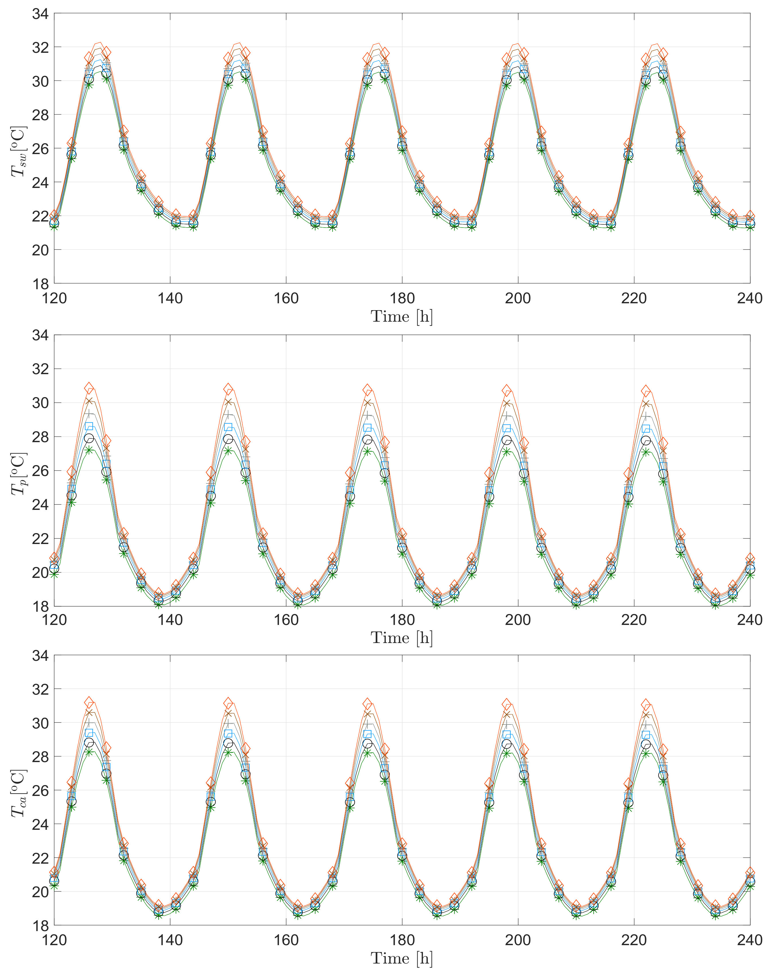
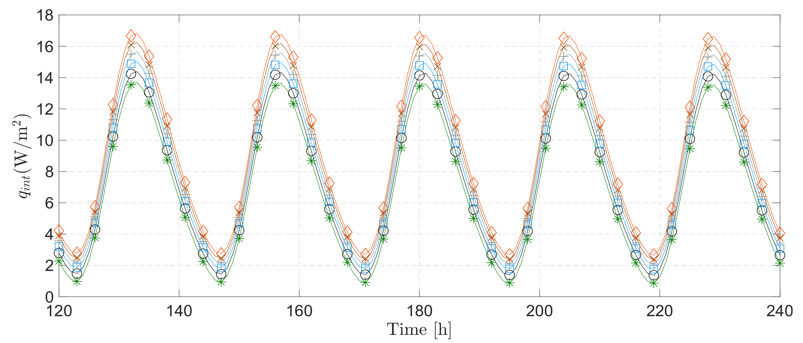
Using the presented numerical model, the sensitivity of natural, mixed and forced convection heat exchange from the bare brick and vegetated brick wall surface and the ambient to different wind velocities, v (0.0 m/s, 0.5 m/s, 1.5 m/s, 2.5 m/s, 3.5 m/s, and 4.5 m/s), was analysed first, whilst all other model parameters were kept constant. Increasing the wind speed on the bare facade during the day had a dominant impact on reducing the exterior facade temperature $T_{sw}$ and indoor heat flux $q_{int}$ through the porous brick wall. During the night, the impact is less noticeable and can be ignored, as shown in Figure 2 and Figure 3.

For the tested modelled range in wind velocities, the maximum bare facade surface temperatures, $T_{sw}$, were $56.0{}^{\circ }$C, $55.9{}^{\circ }$C, $52.6{}^{\circ }$C, $49.8{}^{\circ }$C, $47.6{}^{\circ }$C, and $45.9{}^{\circ }$C, whilst the corresponding indoor heat flux values were in the range from $q_{int}=54.9$ W/m${}^2$ to $q_{int}=36.8$ W/m${}^2$(see

Table 2. Maximum indoor heat fluxes $q_{int}$ (W/m${}^2$) through the porous brick wall without and with vegetation.

Wind Speed (m/s)	Bare Facade	Vegetated Facade
0.0	54.9	21.6
0.5	54.6	16.6
1.5	48.4	14.9
2.5	43.3	14.5
3.5	39.6	14.3
4.5	36.8	14.2

). The numerical simulation results for the vegetated facade are depicted in Figure 4 and Figure 5. It is evident that the foliage had beneficial effects on the hygrothermal behaviour of the facade by lowering the maximum temperatures, $T_{sw}$ ($35.7{}^{\circ }$C, $32.5{}^{\circ }$C, $31.5{}^{\circ }$C, $31.2{}^{\circ }$C, $31.1{}^{\circ }$C, $31.0{}^{\circ }$C), and consequently the corresponding heat load values on the indoor wall were significantly reduced in the range from $q_{int}=21.6$ W/m${}^2$ to $q_{int}=14.2$ W/m${}^2$ (see Table 2).

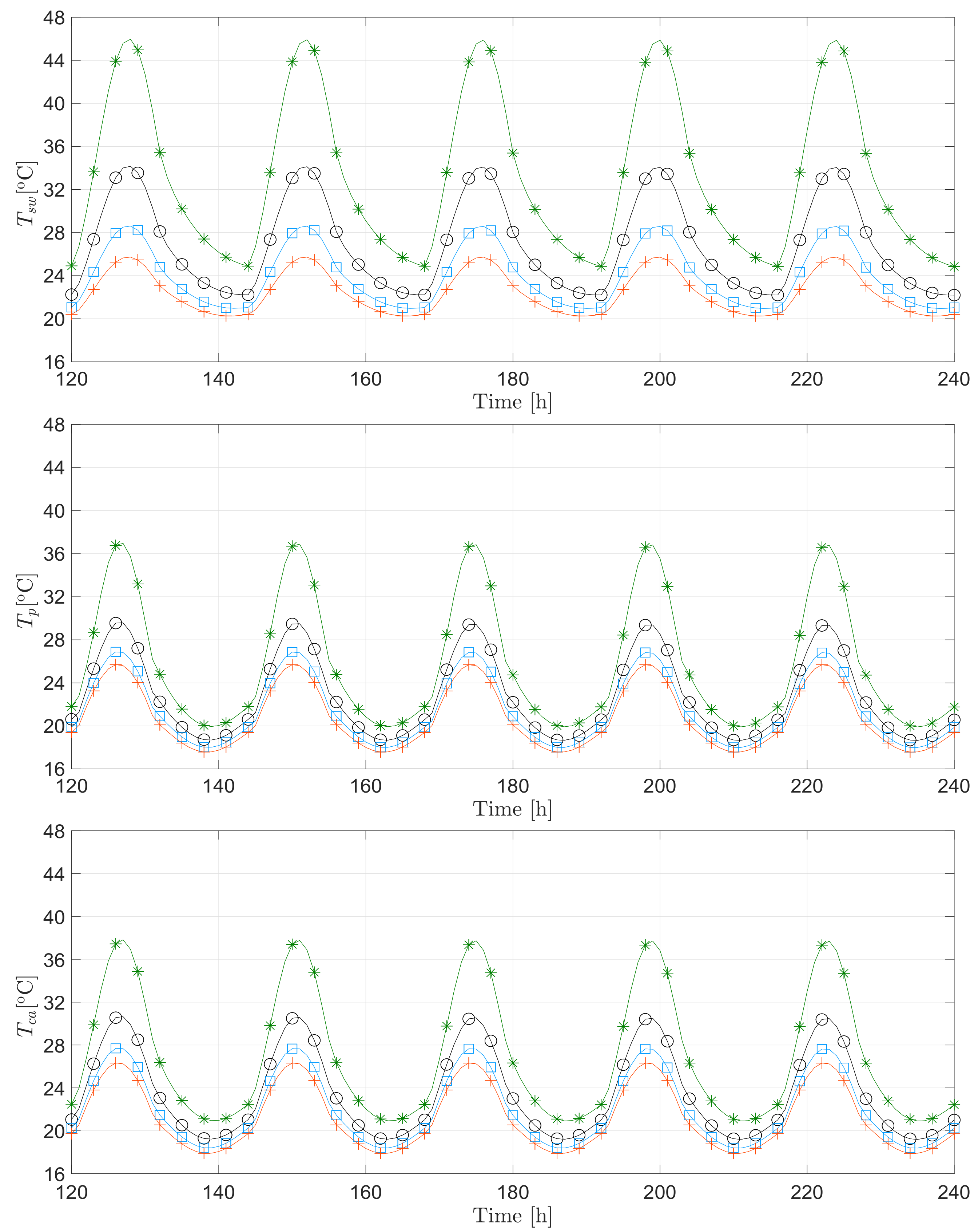
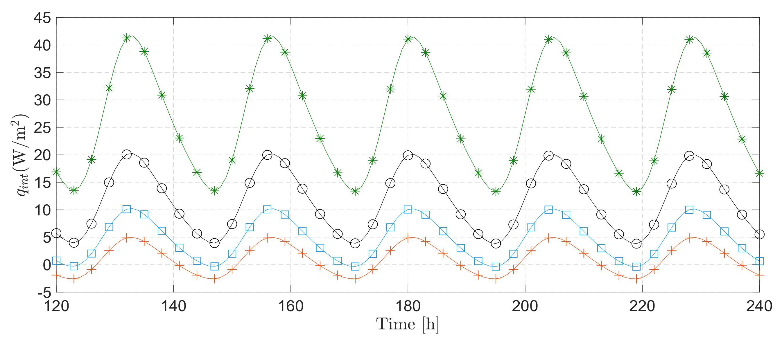
Numerous canopy parameters have significant impacts on the hydrothermal performance of the vegetated facades, including minimum stomatal resistance ($r_{i,min}$), leaf area index ($LAI$), shortwave extinction coefficient ($k_s$), etc.

The cooling effect of the transpiration heat flux from the leaves was evaluated by changing the values of a minimum stomatal resistance $r_{i,min}$ in the range (80 s/m, 120 s/m, 160 s/m, 200 s/m, 240 s/m, 280 s/m), shown in Figure 6 and Figure 7. The biggest difference in facade surface temperature for the maximum and minimum resistance, $r_{i,min}$, is approximately $\mathsf{\Delta }{T}_{sw}\approx 1.8{}^{\circ }$C, with the corresponding approximate difference in indoor heat flux $\mathsf{\Delta }{q}_{int}\approx 3.2$ W/m${}^2$.

Besides the wind velocity and the ambient temperature, shortwave solar radiation is one of the most crucial weather parameters that affects the behaviour of green walls. A canopy absorbs a fraction of incident solar radiation and transmits the rest through the greenery system. The transmittance of the solar radiation through the canopy exponentially decreases with foliage density, given by Equation (9), where the attenuating effect is expressed through an extinction/attenuation coefficient, $k_s$, and a leaf area index, $LAI$. Figure 8, Figure 9, Figure 10 and Figure 11 show the impact of various $LAI$ and $k_s$ values on the hygrothermal behaviour of the vegetated wall. Increasing the leaf area index $LAI$ values and the extinction coefficient $k_s$ values, the facade surface temperature and the heat flux through the structure porous wall decrease significantly. A dense canopy with a $LAI>3$ and with $k_s>0.7$ (leaves parallel to the wall) is particularly effective in reducing the facade surface temperature $T_{sw}$ and heat flux load $q_{int}$.

5.2. Four-Layer Greenery System (Canopy-ICB-Mortar-Concrete Wall Model)

This example represents a single concrete wall, initially built without thermal insulation, but later coated with a layer of insulation after the interposition of a mortar water-proofing layer. As can be seen in the example above, the vegetation climbs along it with the roots on the ground.

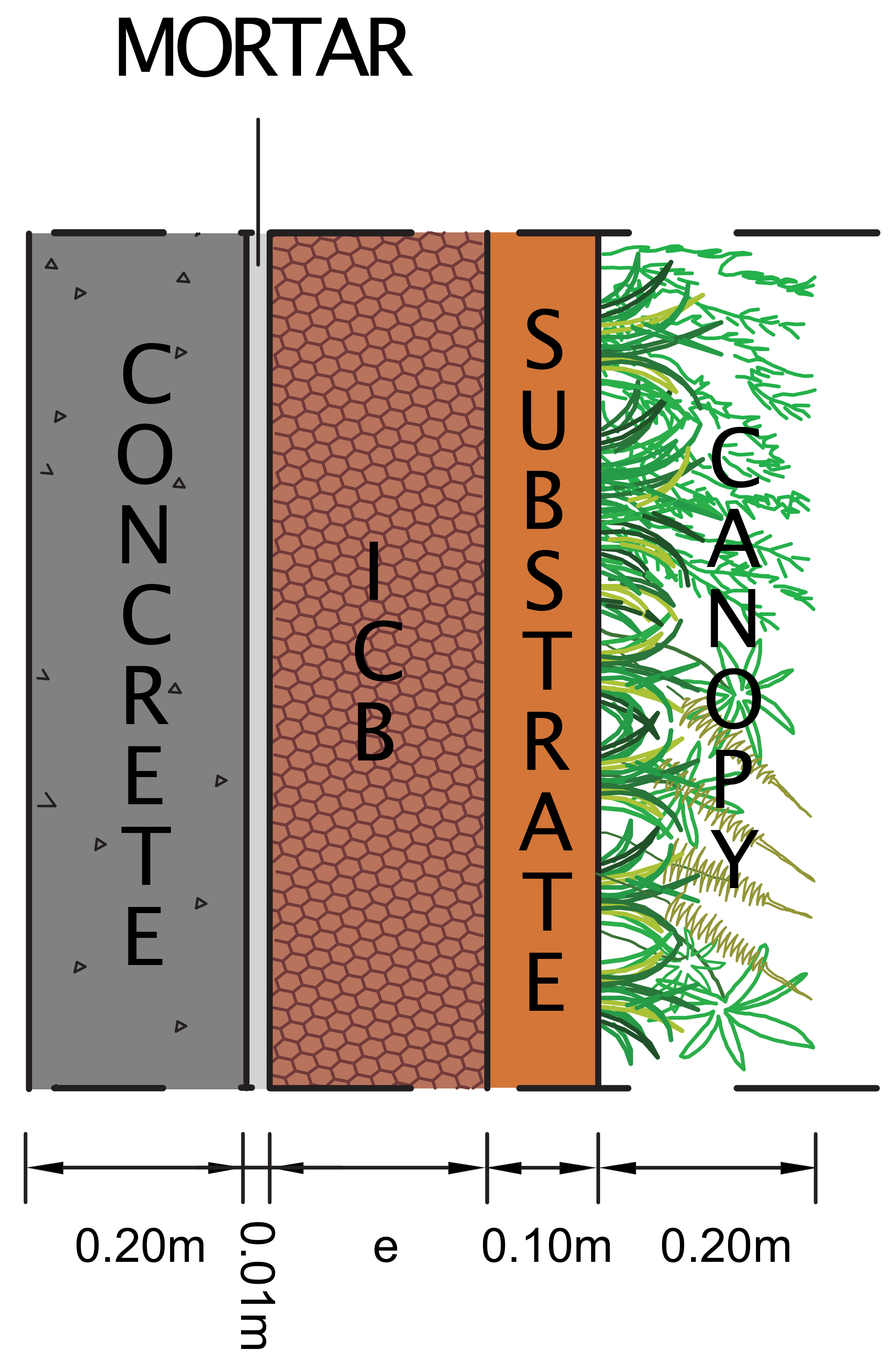
The realistic direct green wall system, a schematic representation of which is depicted in Figure 12, considers the heat and moisture transport in a four-layer canopy–ICB–mortar–concrete structure, where the thickness of the individual layers are: canopy, ${\delta }_c$ (0.20 m); ICB, ${\delta }_{ICB}$ (0.00 m, 0.05 m, 0.10 m, 0.15 m, and 0.20 m); mortar, ${\delta }_m$ (0.01 m); and concrete, ${\delta }_{co}$ (0.20 m). This system was exposed to the periodic fluctuation of the prevailing weather conditions given by Equations (40) and (41).

The time-dependent simulation was performed by running the computation from the initial thermodynamic state with a time-step value $\mathsf{\Delta }t=1800$ s. The simulation time was 240 h (however, the results are only plotted from $t=120$ h to $t=240$ h to allow an easy interpretation of the plots). Two non-uniform density macro-element meshes of M = $45\times 1$ and M = $75\times 1$ were applied to numerically solve a highly nonlinear coupled transport of heat and moisture through the multilayered system. The first (coarser) one adequately captured the transport phenomena in the systems with the canopy, while for the cases without the canopy, only the finer mesh was good enough, since the nonlinearity in moisture transport became more severe.

The influence of the canopy on the multilayered system with two different thicknesses of the medium density expanded cork (ICB), namely ${\delta }_{ICB}=0.10$ m and ${\delta }_{ICB}=0.15$ m, is depicted in Figure 13. It is evident that the canopy reduces the heat load on the interior side in both cases of insulation thickness, although the increasing thickness of the ICB insulation material has a greater impact. We can say that in the multilayer greenery system the influence of the insulation as well as the canopy on reducing the thermal load of the interior is significant. However, it is also clearly shown that the canopy acts mainly as the solar radiation barrier, namely by increasing the shortwave radiation extinction coefficient from the value $k_s=0.6$ to the value $k_s=0.9$, such that the reduction of heat load on the interior is most noticeable.

Figure 14 illustrates how the driving potentials, such as relative humidity $\phi (t,x)$, water content $W(t,x)$, and temperature $T(t,x)$, change with time (t = 216, 222, 228 and 234 h) throughout the multilayer wall cross section. The bare and the vegetated facades were analysed for the ${\delta }_{ICB}$ = 0.10 m thick ICB insulation layer. During sun exposure, the bare facade exterior surface temperature rose as high as T $\approx 54{}^{\circ }$C, whilst the maximum ambient temperature was T $=33{}^{\circ }$C; the solar heat radiation is absorbed and stored by the exterior ICB surface. Due to very low heat diffusivity of the ICB material, the propagation of heat from the surface to the interior is very slow, resulting in a high surface temperature. Large surface temperature fluctuations result at the same time in large fluctuations of surface relative humidity. The slow moisture diffusion process means the fluctuations are limited to the wall surface. In fact, the exterior surface temperature of the vegetated facade is much lower, T $\approx 45{}^{\circ }$C for $K_s=0.6$ and T $\approx 34{}^{\circ }$C for $K_s=0.9$, suggesting that the choice of suitable plants for the canopy is of crucial importance. It can be also noted that the computed difference in the surface night temperature between the bare and vegetated facade is negligible. Heat convection is the dominant heat transfer mechanism and the ambient temperature controlled the facade surface temperature. The longwave heat radiation from the bare facade is slightly more intense, which resulted in a lower night surface temperature.

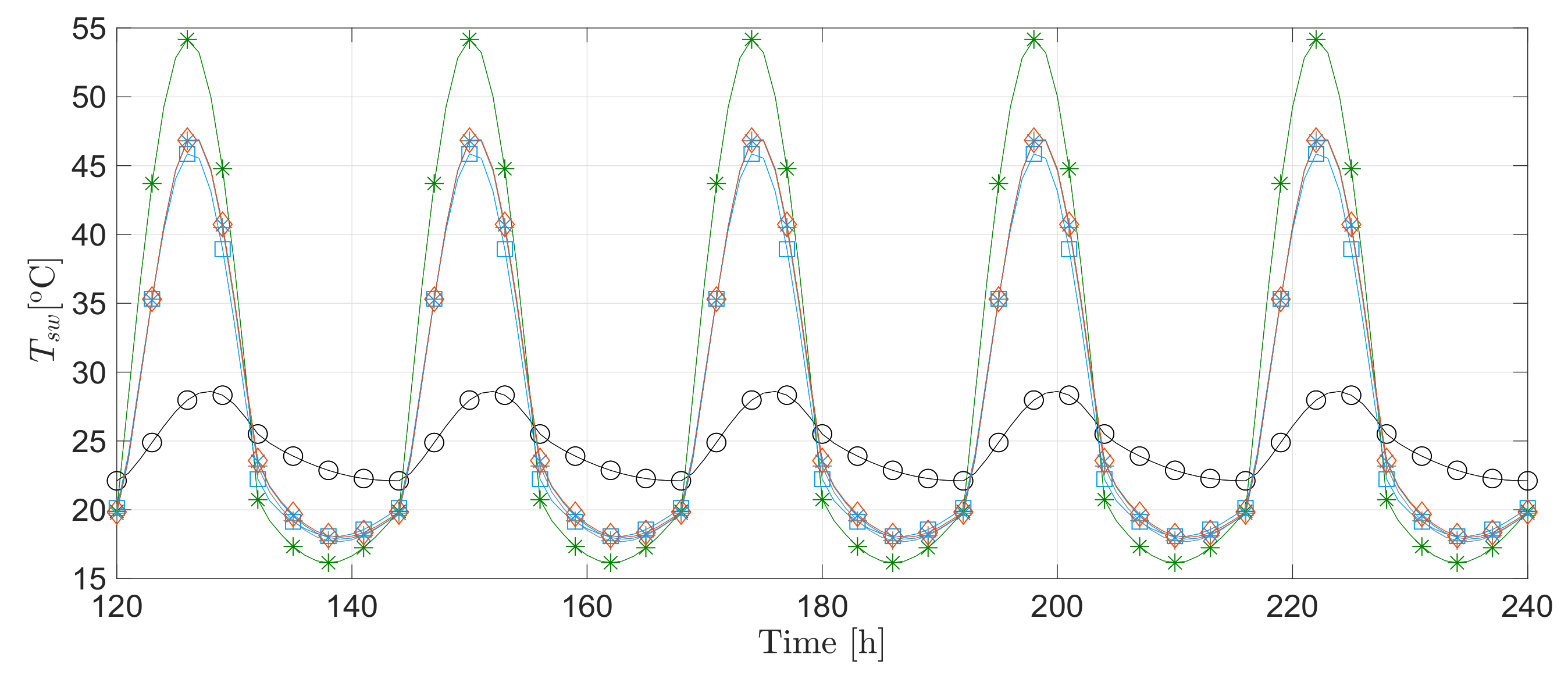
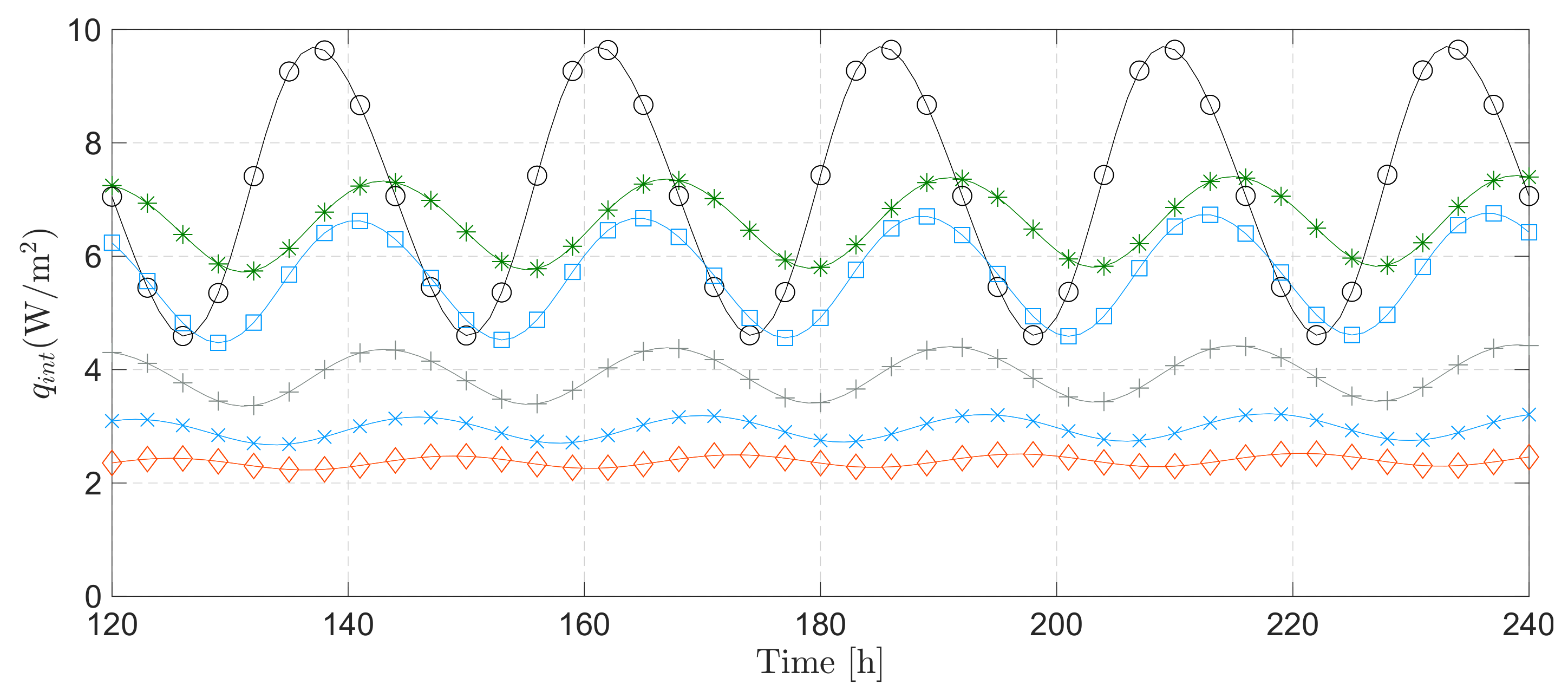
Figure 15 and Figure 16 give the time variations of the heat load at the inner surface of the wall and temperature at the external surface. It is evident that the system without the ICB layer leads to the highest heat load of the interior. Simultaneously, the daytime external surface temperature is the lowest due to the high heat diffusivity coefficients of mortar and concrete.

5.3. Five-Layer Greenery System (Canopy–Substrate–ICB–Mortar–Concrete System)

As before, this example represents a single concrete wall, initially built without thermal insulation, but later given an insulating layer, after the placement of a mortar water-proofing layer. However, the vegetation now grows on a substrate layer superimposed to the insulating layer.

This green wall, represented inFigure 17, considers the heat and moisture transport in a five-layer system composed of canopy–substrate–ICB–mortar–concrete: canopy, ${\delta }_c$ (0.20 m); substrate, ${\delta }_s$ (0.10 m); ICB, ${\delta }_{ICB}$ (0.00 m, 0.05 m, 0.10 m, 0.15 m, and 0.20 m); mortar, ${\delta }_m$ (0.01 m); and concrete, ${\delta }_{co}$ (0.20 m). The system was exposed to the periodic fluctuation of the prevailing ambient parameters. Boundary and initial conditions were taken to be the same as those previously prescribed by Equations (39)–(41), with the exception that the initial conditions for the substrate relative humidity were equated to value $\phi =0.95$. The substrate/clay loam soil thermohydraulic properties were taken from the literature [33].

Numerous time-dependent analyses of transport phenomena in a multilayer structure were performed by running the simulations from the initial state with a time-step value $\mathsf{\Delta }t=1800$ s; the simulation time was 240 h (as before, the results are only plotted from $t=120$ h to $t=240$ h to allow an easy interpretation of the plots). Non-uniform density macro-element meshes of M = $75\times 1$, M = $100\times 1$ and M = $115\times 1$ were applied to numerically model a highly nonlinear coupled transport of heat and moisture through the canopy, substrate, ICB, mortar and concrete layer; to cope with the severe nonlinearity of the outer layer/substrate 50 macro-elements were used.

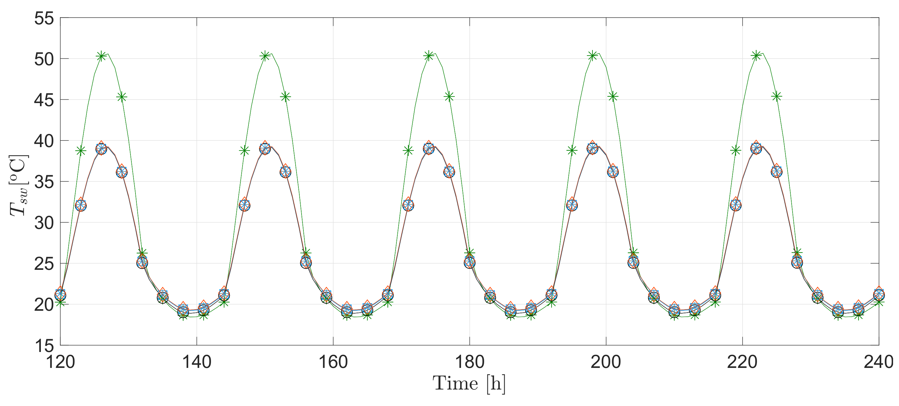
Figure 18 and Figure 19 present the time variations of the heat flux at the interior surface of the wall and temperature at the external surface as a function of ICB thickness; the thickness of the substrate layer was kept constant at ${\delta }_s=0.10$ m. Comparing these results with those shown in Figure 15 and Figure 16, it can be concluded that a substrate layer considerably reduces heat flux through the multilayer wall and the facade surface temperature. Overall, the maximum surface temperature of the vegetated facade is $T_{sw}\approx 38{}^{\circ }$C, regardless of ICB insulation layer thickness. This is because of the favourable thermohydraulic properties of the soil in terms of heat diffusion when compared to ICB.

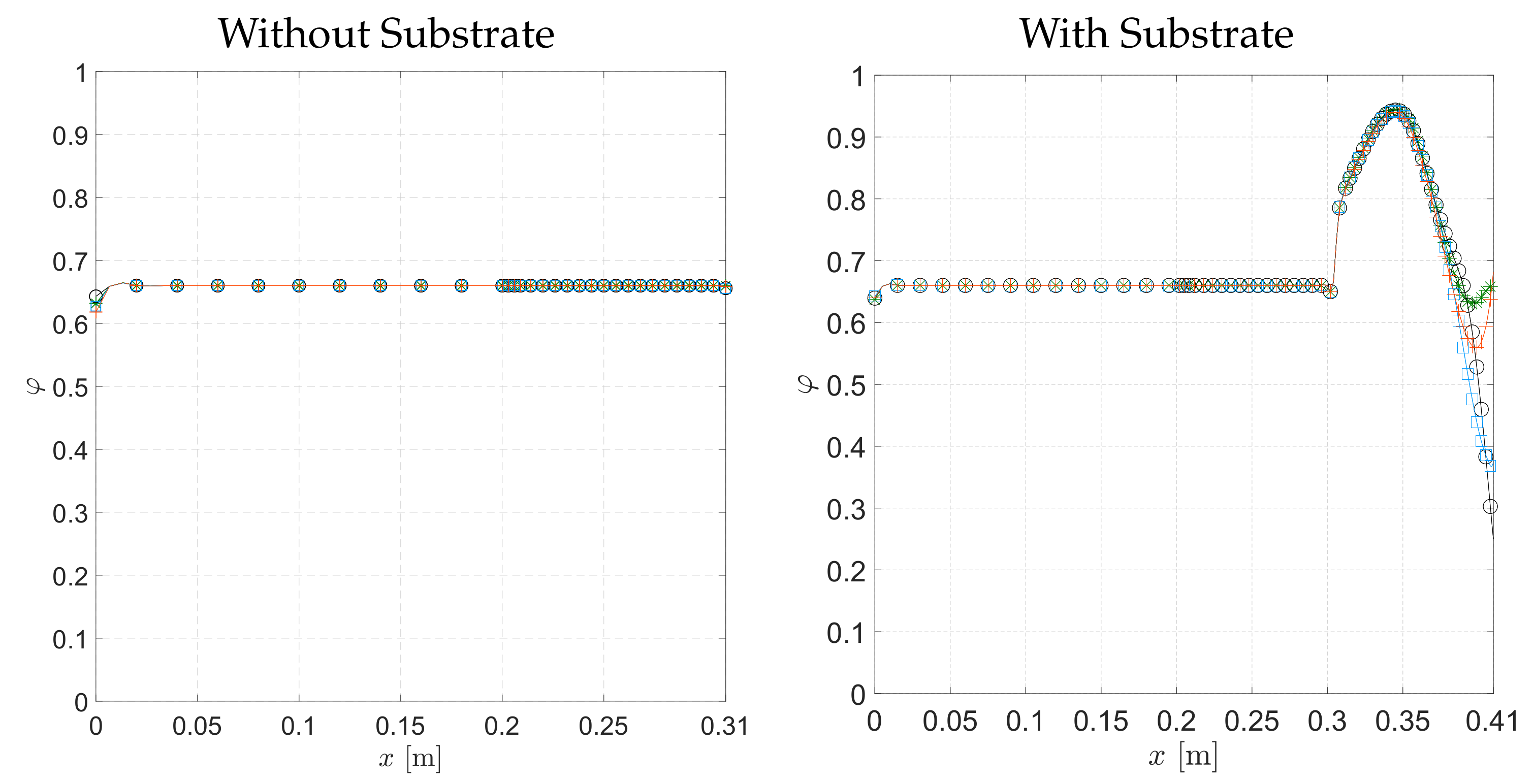
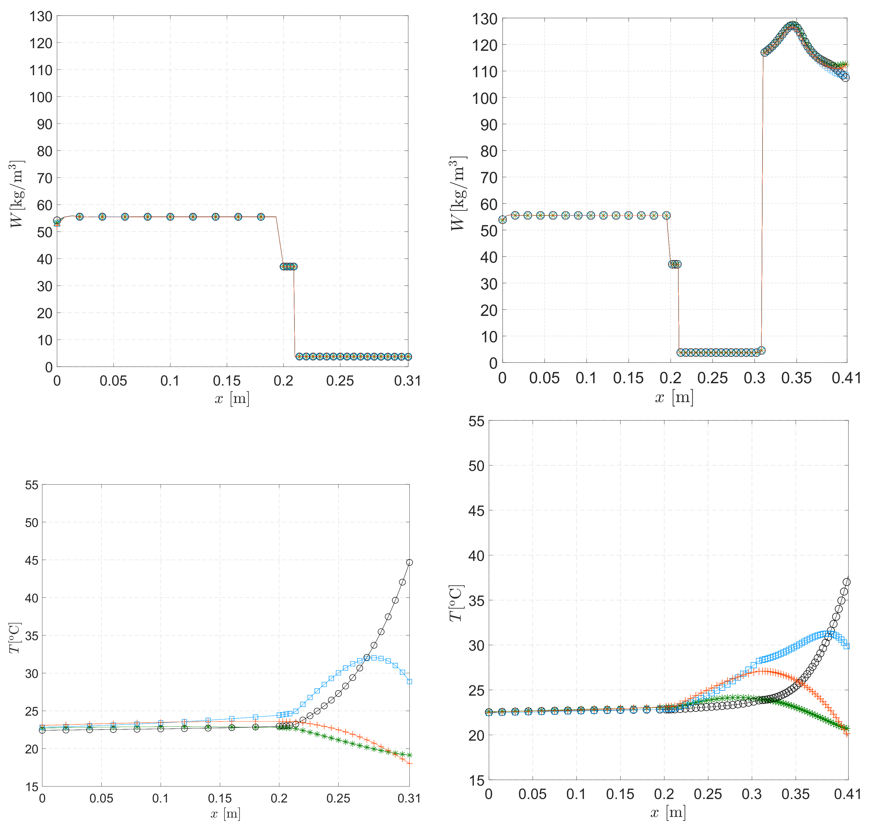
Figure 20 illustrates the time dependence of the driving potentials (t = 216, 222, 228 and 234 h), such as the relative humidity $\phi (t,x)$, water content $W(t,x)$, and temperature $T(t,x)$ throughout the multilayer wall cross section with and without substrate.

6. Conclusions

In this contribution, the numerical simulation tool governing the transport phenomena in green roofs [11] was modified in such a way as to be able to estimate the transport of heat and moisture in vegetated vertical walls. The proposed numerical solution procedure deals with the highly nonlinear coupled heat and moisture transport through a multilayer structure composed of a canopy and a support structure. The relevant physical–mathematical models governing the transfer of heat and moisture through the canopy and porous solid media have been discussed. The required empiricism to close the mathematical models has been considered, too. The respective boundary and interface conditions, and the coupling between the canopy and the facade surface were then formulated.

A standard first and second order finite difference FDM scheme was used to numerically solve the ODEs governing the transport phenomenon through the canopy layer, whilst the PDEs that govern the transport phenomenon through the porous solid material layers are solved with the boundary element numerical model (BEM). The finite difference and singular integral representations of the respective ODEs and PDEs were considered. The basic idea of transforming the integral equations to the boundary element numerical model has also been presented briefly. We have considered a very accurate numerical scheme based on quadratic approximations of all relevant field functions over the space domain, and linear over time.

The presented numerical simulation tool can be used to quantify the dependence of the heat load on various influential parameters of the vegetated systems, such as the parameters defined for the canopy and the structural parameters of the multilayer wall. Several test multilayer wall cases were analysed to prove the capability and the sensitivity of the developed model.

Based on the analysis of the simulation results presented in this contribution and results taken from the literature, some conclusions can be established. The local environmental conditions, i.e., wind velocity, temperature and shortwave solar radiation, are the most critical influential parameters. The density of the canopy (LAI) and the orientation of the leaves also have a dominant influence on the transmittance of solar radiation, and thus on the facade surface temperature and heat flux load. The cooling effect of transpiration, governed by the stomatal internal leaf resistance, is noticeable as well. Additionally, the influence of different parameters is more pronounced during the day than at night.

Ultimately, the developed model is a compromise engineering tool to assess very complex transport phenomena through the greenery system based on the extended empiricism, which should be further tested and improved.