
On the Evaluation of Interfacial Tension (IFT) of CO2–Paraffin System for Enhanced Oil Recovery Process: Comparison of Empirical Correlations, Soft Computing Approaches, and Parachor Model

 ,
,  , and
, and 
Abstract

1. Introduction
2. Data Collection
3. Model Development
3.1. Multilayer Perceptron (MLP) Neural Networks
3.2. Radial Basis Function (RBF) Neural Networks
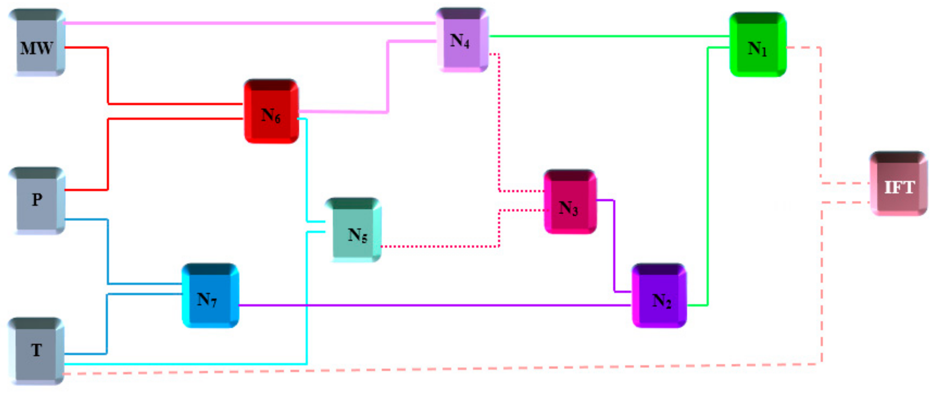
3.3. Group Method of Data Handling (GMDH)
4. Results and Discussion
4.1. Accuracy and Validity of the Models

| Model | APRE, % | AAPRE, % | RMSE, mN/m | R2 | SD | |
|---|---|---|---|---|---|---|
| RBF-ICA | Train | −1.49 | 4.43 | 0.53 | 0.99 | 0.02 |
| Test | −1.40 | 4.35 | 0.57 | 0.99 | 0.01 | |
| Total | −1.47 | 4.42 | 0.54 | 0.99 | 0.02 | |
| Train | −0.62 | 5.07 | 0.57 | 0.99 | 0.01 | |
| RBF-GA | Test | −2.51 | 5.35 | 0.44 | 0.99 | 0.03 |
| Total | −1.00 | 5.12 | 0.55 | 0.99 | 0.02 | |
| RBF-GSA | Train | −1.37 | 5.65 | 0.64 | 0.99 | 0.03 |
| Test | −1.65 | 5.95 | 0.66 | 0.98 | 0.02 | |
| Total | −1.43 | 5.71 | 0.64 | 0.99 | 0.03 | |
| Train | −0.95 | 5.43 | 0.50 | 0.99 | 0.02 | |
| RBF-ACO | Test | −1.38 | 7.52 | 0.78 | 0.98 | 0.02 |
| Total | −1.02 | 5.85 | 0.57 | 0.99 | 0.02 | |
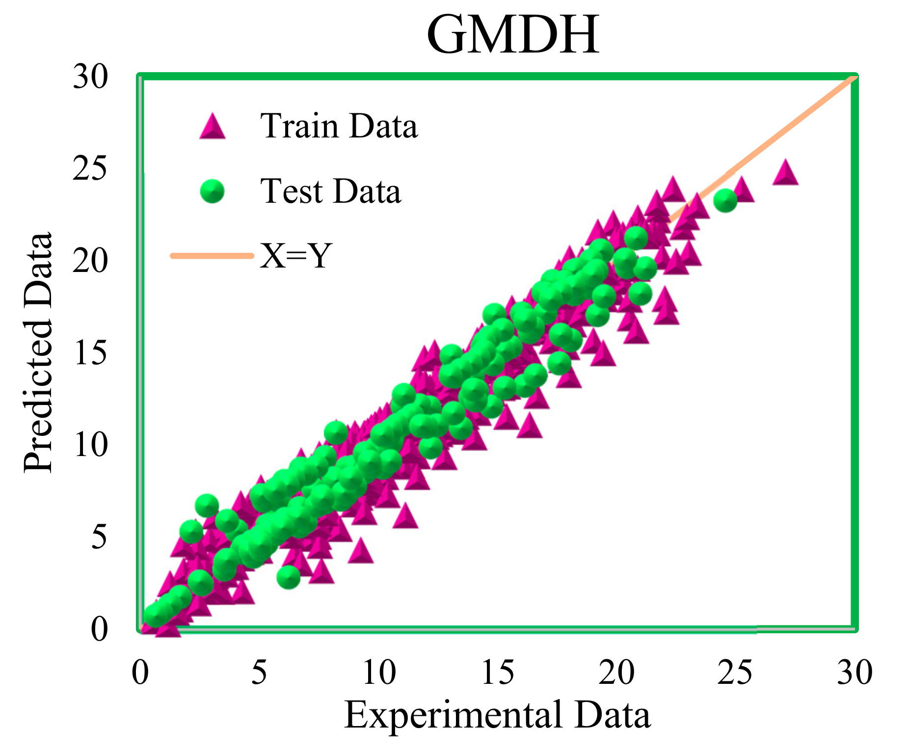
| Train | −1.62 | 9.65 | 1.05 | 0.95 | 0.05 | |
| GMDH | Test | −3.49 | 10.52 | 0.99 | 0.96 | 0.03 |
| Total | −2.00 | 9.81 | 1.03 | 0.95 | 0.02 | |
| Train | −2.06 | 9.87 | 0.80 | 0.98 | 0.05 | |
| RBF-PSO | Test | −3.19 | 12.36 | 1.15 | 0.95 | 0.05 |
| Total | −2.28 | 10.37 | 0.88 | 0.97 | 0.05 | |
| Train | −3.08 | 11.97 | 1.18 | 0.95 | 0.05 | |
| MLP-LM | Test | −2.19 | 13.88 | 1.31 | 0.94 | 0.07 |
| Total | −2.93 | 12.49 | 1.23 | 0.95 | 0.07 |
4.2. Analyzing Trend of RBF-ICA Outcomes
4.3. Sensitivity Analysis
4.4. Outlier Detection
4.5. Comparison between Proposed and Pre-Existing Models
5. Conclusions
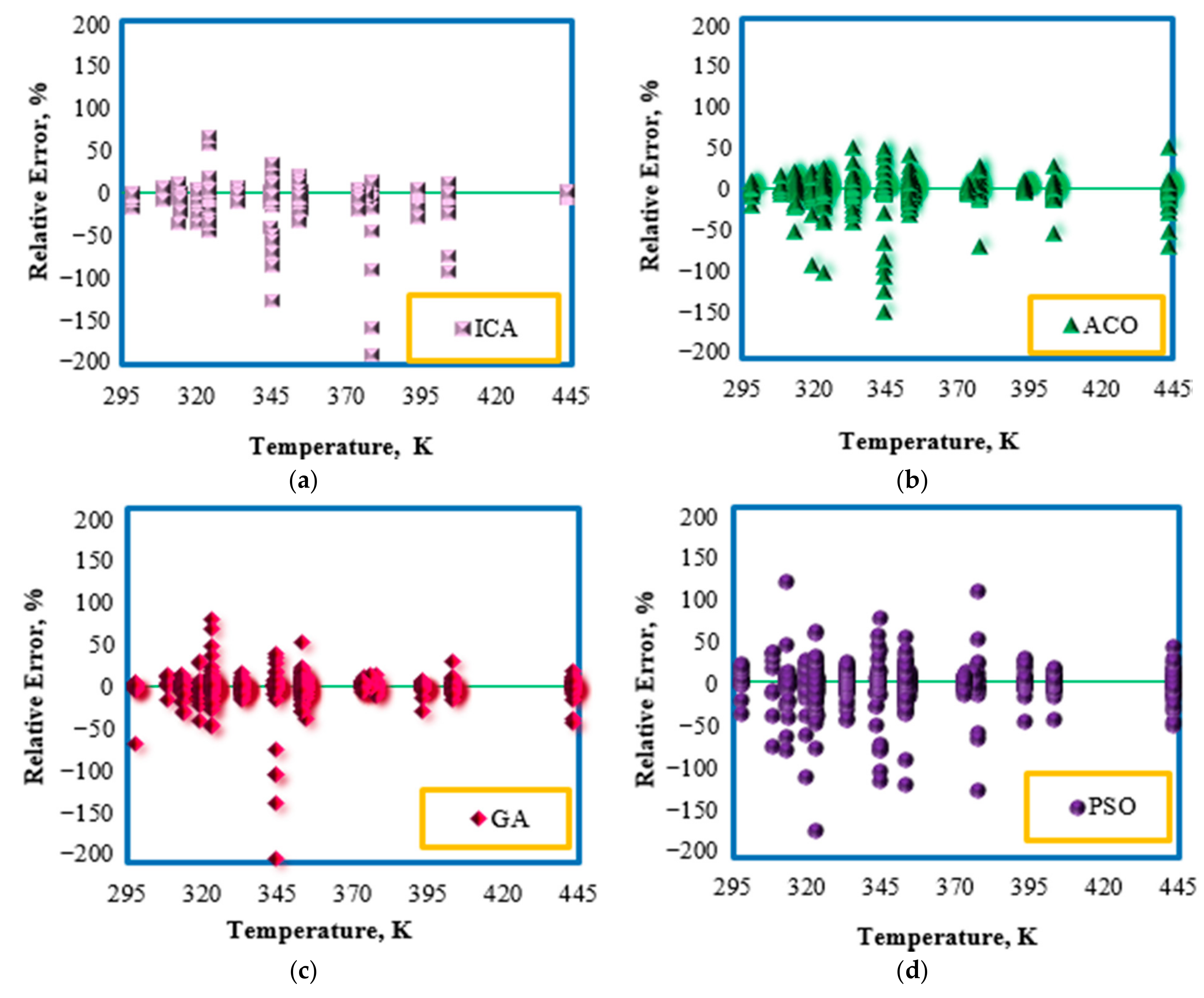
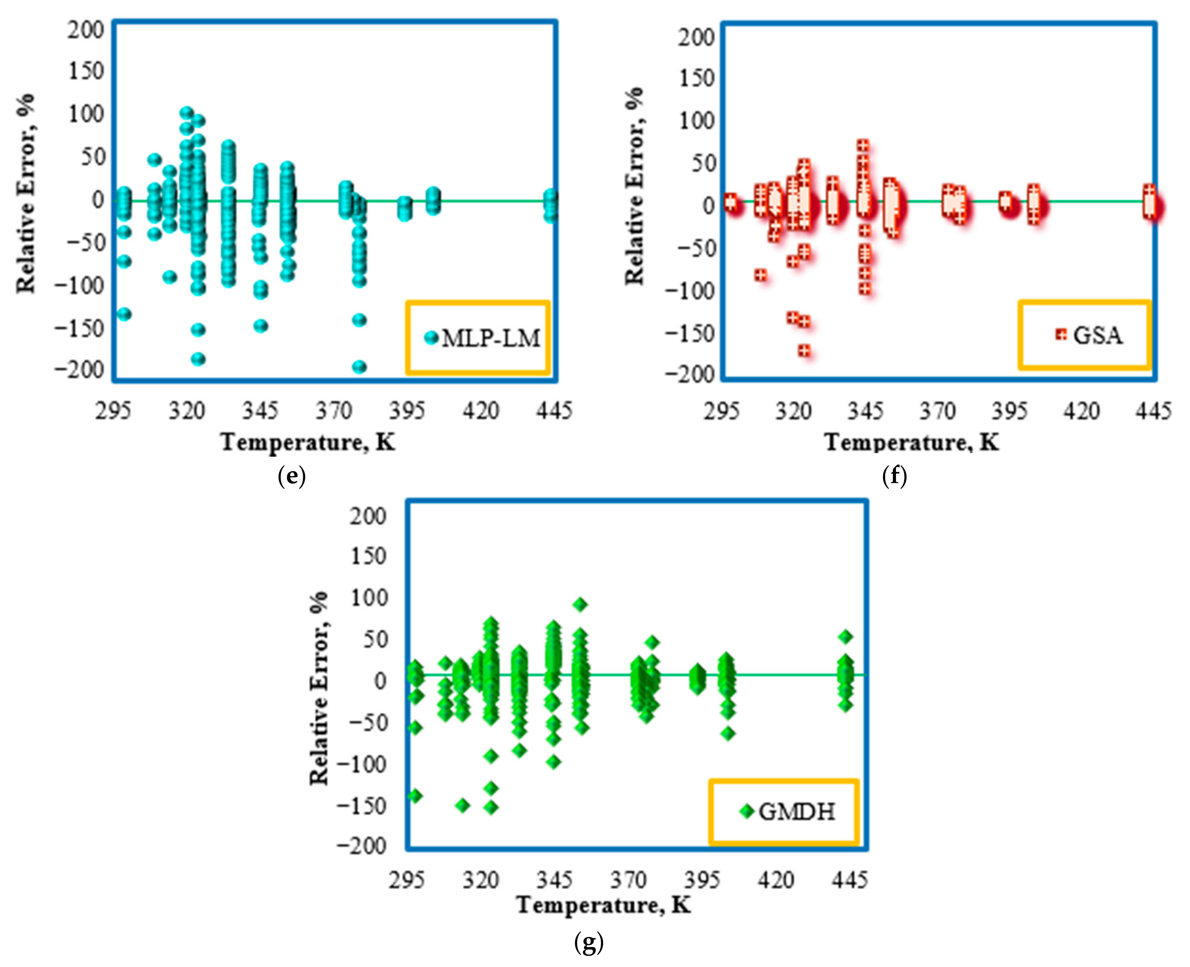
- All the developed models for IFT prediction of the CO2–n-alkane systems yielded accurate results both for the training stage and the testing stage. The proposed techniques could be sorted in decreasing order of accuracy as follows:
- RBF-ICA > RBF-GA > RBF-GSA > RBF-ACO > GMDH > RBF-PSO > MLP-LM.
- The expected physical trends for the CO2–n-alkane systems were successfully followed, and the effects of pressure, temperature, and MW of n-alkanes on IFT behavior of the targeted systems were thoroughly studied.
- The higher value of the relevancy factor for pressure, in comparison with the values for temperature and MW of n-alkane, implied the significant impact of the pressure on the IFT of the CO2–n-alkane.
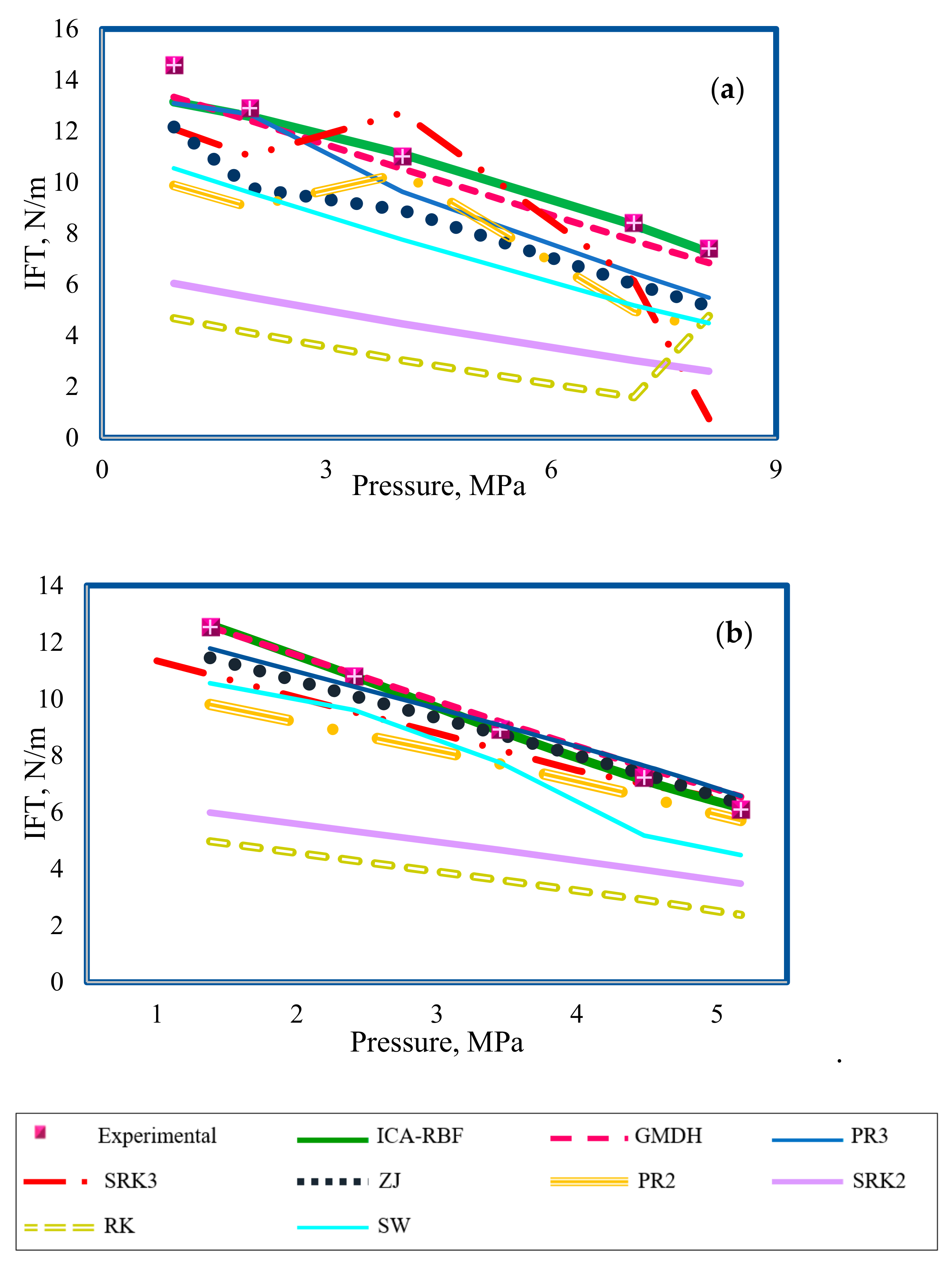
- By comparing the performance of the RBF-ICA, GMDH, and Parachor models in IFT estimation of the CO2–n-heptane and CO2–n-decane systems, the superiority of the RBF-ICA model over the other models was obvious. After that, the GMDH model, followed by the Parachor equation () combined with the PR3, SRK3, and ZJ EOSs, showed an excellent match with the experimental data for the aforementioned binary systems.
- From a statistical viewpoint, both the used laboratory data and the developed models were valid. Only 1.9% of the used data were out of the applicability domain of the suggested RBF-ICA model, proving the high accuracy of the model.
Supplementary Materials
Author Contributions
Funding
Institutional Review Board Statement
Informed Consent Statement
Data Availability Statement
Conflicts of Interest
References
- Moeini, F.; Hemmati-Sarapardeh, A.; Ghazanfari, M.-H.; Masihi, M.; Ayatollahi, S. Toward mechanistic understanding of heavy crude oil/brine interfacial tension: The roles of salinity, temperature and pressure. Fluid Phase Equilibria 2014, 375, 191–200. [Google Scholar] [CrossRef]
- Derikvand, Z.; Rezaei, A.; Parsaei, R.; Riazi, M.; Torabi, F. A mechanistic experimental study on the combined effect of Mg2+, Ca2+, and SO42− ions and a cationic surfactant in improving the surface properties of oil/water/rock system. Colloids Surf. A Phys. Eng. Asp. 2020, 587, 124327. [Google Scholar] [CrossRef]
- Rezaei, A.; Riazi, M.; Escrochi, M. Investment Opportunities in Iranian EOR Projects; European Association of Geoscientists & Engineers. St. Petersburg 2018 2018. [Google Scholar] [CrossRef]
- Rezaei, A.; Riazi, M.; Escrochi, M.; Elhaei, R. Integrating surfactant, alkali and nano-fluid flooding for enhanced oil recovery: A mechanistic experimental study of novel chemical combinations. J. Mol. Liq. 2020, 308, 113106. [Google Scholar] [CrossRef]
- Yazdanpanah, A.; Rezaei, A.; Mahdiyar, H.; Kalantariasl, A. Development of an efficient hybrid GA-PSO approach applicable for well placement optimization. Adv. Geo Energy Res. 2019, 3, 365–374. [Google Scholar] [CrossRef]
- Lake, L.W.; Johns, R.T.; Rossen, W.R.; Pope, G.A. Fundamentals of Enhanced Oil Recovery; Society of Petroleum Engineers: Richardson, TX, USA, 2014. [Google Scholar]
- Green, D.W.; Willhite, G.P. Enhanced Oil Recovery; Henry L. Doherty Memorial Fund of AIME, Society of Petroleum Engineers: Richardson, TX, USA, 1998; Volume 6. [Google Scholar]
- Belhaj, H.; Abukhalifeh, H.; Javid, K. Miscible oil recovery utilizing N2 and/or HC gases in CO2 injection. J. Pet. Sci. Eng. 2013, 111, 144–152. [Google Scholar] [CrossRef]
- Fazlali, A.; Nikookar, M.; Mohammadi, A.H. Computational procedure for determination of minimum miscibility pressure of reservoir oil. Fuel 2013, 106, 707–711. [Google Scholar] [CrossRef]
- Hemmati-Sarapardeh, A.; Mohagheghian, E. Modeling interfacial tension and minimum miscibility pressure in paraffin-nitrogen systems: Application to gas injection processes. Fuel 2017, 205, 80–89. [Google Scholar] [CrossRef]
- Khelifa, T.; Maini, B.B. Evaluation of CO2 Based Vapex Process for the Recovery of Bitumen from Tar Sand Reservoirs. In All Days; Society of Petroleum Engineers (SPE): Richardson, TX, USA, 2003. [Google Scholar]
- Aycaguer, A.-C.; Lev-On, A.M.; Winer, A.M. Reducing Carbon Dioxide Emissions with Enhanced Oil Recovery Projects: A Life Cycle Assessment Approach. Energy Fuels 2001, 15, 303–308. [Google Scholar] [CrossRef]
- Soltanian, M.R.; Amooie, M.A.; Cole, D.R.; Graham, D.E.; Hosseini, S.A.; Hovorka, S.; Pfiffner, S.M.; Phelps, T.J.; Moortgat, J. Simulating the Cranfield geological carbon sequestration project with high-resolution static models and an accurate equation of state. Int. J. Greenh. Gas Control 2016, 54, 282–296. [Google Scholar] [CrossRef]
- Ampomah, W.; Balch, R.; Cather, M.; Rose-Coss, D.; Dai, Z.; Heath, J.; Dewers, T.; Mozley, P. Evaluation of CO2 Storage Mechanisms in CO2 Enhanced Oil Recovery Sites: Application to Morrow Sandstone Reservoir. Energy Fuels 2016, 30, 8545–8555. [Google Scholar] [CrossRef]
- Gershenzon, N.I.; Soltanian, M.; Ritzi, R.W.; Dominic, D.F. Understanding the impact of open-framework conglomerates on water–oil displacements: The Victor interval of the Ivishak Reservoir, Prudhoe Bay Field, Alaska. Pet. Geosci. 2014, 21, 43–54. [Google Scholar] [CrossRef]
- Hemmati-Sarapardeh, A.; Ayatollahi, S.; Ghazanfari, M.-H.; Masihi, M. Experimental Determination of Interfacial Tension and Miscibility of the CO2–Crude Oil System; Temperature, Pressure, and Composition Effects. J. Chem. Eng. Data 2014, 59, 61–69. [Google Scholar] [CrossRef]
- Cronin, M.; Emami-Meybodi, H.; Johns, R. Multicomponent Diffusion Modeling of Cyclic Solvent Injection in Ultratight Reservoirs. In SPE Annual Technical Conference and Exhibition; Society of Petroleum Engineers: Richardson, TX, USA, 2019. [Google Scholar]
- Ghasemi, M.; Astutik, W.; Alavian, S.A.; Whitson, C.H.; Sigalas, L.; Olsen, D.; Suicmez, V.S. Determining Diffusion Coefficients for Carbon Dioxide Injection in Oil-Saturated Chalk by Use of a Constant-Volume-Diffusion Method. SPE J. 2017, 22, 505–520. [Google Scholar] [CrossRef]
- Guo, P.; Wang, Z.; Shen, P.; Du, J. Molecular diffusion coefficients of the multicomponent gas− crude oil systems under high tem-perature and pressure. Ind. Eng. Chem. Res. 2009, 48, 9023–9027. [Google Scholar] [CrossRef]
- Hoteit, H. Modeling diffusion and gas–oil mass transfer in fractured reservoirs. J. Pet. Sci. Eng. 2013, 105, 1–17. [Google Scholar] [CrossRef]
- Hoteit, H.; Firoozabadi, A. Numerical Modeling of Diffusion in Fractured Media for Gas-Injection and -Recycling Schemes. SPE J. 2009, 14, 323–337. [Google Scholar] [CrossRef]
- Shang, Q.; Xia, S.; Cui, G.; Tang, B.; Ma, P. Measurement and correlation of the interfacial tension for paraffin + CO2 and (CO2 +N2) mixture gas at elevated temperatures and pressures. Fluid Phase Equilibria 2017, 439, 18–23. [Google Scholar] [CrossRef]
- Karkevandi-Talkhooncheh, A.; Hajirezaie, S.; Hemmati-Sarapardeh, A.; Husein, M.M.; Karan, K.; Sharifi, M. Application of adaptive neuro fuzzy interface system optimized with evolutionary algorithms for modeling CO2 -crude oil minimum miscibility pressure. Fuel 2017, 205, 34–45. [Google Scholar] [CrossRef]
- Barati-Harooni, A.; Najafi-Marghmaleki, A.; Hoseinpour, S.-A.; Tatar, A.; Karkevandi-Talkhooncheh, A.; Hemmati-Sarapardeh, A.; Mohammadi, A.H. Estimation of minimum miscibility pressure (MMP) in enhanced oil recovery (EOR) process by N2 flooding using different computational schemes. Fuel 2019, 235, 1455–1474. [Google Scholar] [CrossRef]
- Rezaei, A.; Khodabakhshi, A.; Esmaeili, A.; Razavifar, M. Effects of initial wettability and different surfactant-silica nanoparticles flooding scenarios on oil-recovery from carbonate rocks. Petroleum 2021. [Google Scholar] [CrossRef]
- Yang, D.; Gu, Y. Interfacial Interactions between Crude Oil and CO2 Under Reservoir Conditions. Pet. Sci. Technol. 2005, 23, 1099–1112. [Google Scholar] [CrossRef]
- Li, H.; Zheng, S.; Yang, D.T. Enhanced swelling effect and viscosity reduction of solvent (s)/CO2/heavy-oil systems. SPE J. 2013, 18, 695–707. [Google Scholar] [CrossRef]
- Hassan, M.E.; Nielsen, R.F.; Calhoun, J.C. Effect of pressure and temperature on oil-water interfacial tensions for a series of hy-drocarbons. J. Pet. Technol. 1953, 5, 299–306. [Google Scholar] [CrossRef]
- Rezaei, A.; Derikvand, Z.; Parsaei, R.; Imanivarnosfaderani, M. Surfactant-silica nanoparticle stabilized N2-foam flooding: A mechanistic study on the effect of surfactant type and temperature. J. Mol. Liq. 2021, 325, 115091. [Google Scholar] [CrossRef]
- Ling, K.; He, J. A New Correlation to Calculate Oil-Water Interfacial Tension. In SPE Kuwait International Petroleum Conference and Exhibition; Society of Petroleum Engineers: Richardson, TX, USA, 2012. [Google Scholar] [CrossRef]
- Adamson, A.W.; Gast, A.P. Physical Chemistry of Surfaces; Interscience: New York, NY, USA, 1967; Volume 15. [Google Scholar]
- Manning, C.D. Measurement of Interfacial Tension: Topical Report; Bartlesville Energy Technology Center: Bartlesville, OK, USA, 1983. [Google Scholar]
- Soori, T.; Rassoulinejad-Mousavi, S.M.; Zhang, L.; Rokoni, A.; Sun, Y. A machine learning approach for estimating surface tension based on pendant drop images. Fluid Phase Equilibria 2021, 538, 113012. [Google Scholar] [CrossRef]
- Dehdari, B.; Parsaei, R.; Riazi, M.; Rezaei, N.; Zendehboudi, S. New insight into foam stability enhancement mechanism, using polyvinyl alcohol (PVA) and nanoparticles. J. Mol. Liq. 2020, 307, 112755. [Google Scholar] [CrossRef]
- Rotenberg, Y.; Boruvka, L.; Neumann, A. Determination of surface tension and contact angle from the shapes of axisymmetric fluid interfaces. J. Colloid Interface Sci. 1983, 93, 169–183. [Google Scholar] [CrossRef]
- Gasem, K.A.M.; Dickson, K.B.; Shaver, R.D.; Robinson, R.L., Jr. Experimental phase densities and interfacial tensions for a CO2/synthetic-oil and a CO2/reservoir-oil system. SPE Reserv. Eng. 1993, 8, 170–174. [Google Scholar] [CrossRef]
- Rao, D.N. A new technique of vanishing interfacial tension for miscibility determination. Fluid Phase Equilibria 1997, 139, 311–324. [Google Scholar] [CrossRef]
- Gasem, K.A.M.; Dickson, K.B.; Dulcamara, P.B.; Nagarajan, N.; Robinson, R.L., Jr. Equilibrium phase compositions, phase densities, and interfacial tensions for carbon dioxide+ hydrocarbon systems. 5. Carbon dioxide+ n-tetradecane. J. Chem. Eng. Data 1989, 34, 191–195. [Google Scholar] [CrossRef]
- Shaver, R.D.; Robinson, R.L., Jr.; Gasem, K.A.M. An automated apparatus for equilibrium phase compositions, densities, and inter-facial tensions: Data for carbon dioxide+ decane. Fluid Phase Equilibria 2001, 179, 43–66. [Google Scholar] [CrossRef]
- Roush, K.V. Automated Phase Densities and Interfacial Tension Measurements. Ph.D. Thesis, Oklahoma State University, Stillwater, OK, USA, 1991. [Google Scholar]
- Jennings, J.W., Jr.; Pallas, N.R. An efficient method for the determination of interfacial tensions from drop profiles. Langmuir 1988, 4, 959–967. [Google Scholar] [CrossRef]
- Carey, B.S. The gradient theory of fluid interfaces. Ph.D. Thesis, Minnesota University, Minneapolis, MN, USA, 1979. [Google Scholar]
- Clever, H.L.; Chase, W.E., Jr. Thermodynamics of Liquid Surfaces. J. Chem. Eng. Data 1963, 8, 291–292. [Google Scholar] [CrossRef]
- Brock, J.R.; Bird, R.B. Surface tension and the principle of corresponding states. AIChE J. 1955, 1, 174–177. [Google Scholar] [CrossRef]
- Sugden, S. VI.—The variation of surface tension with temperature and some related functions. J. Chem. Soc. Trans. 1924, 125, 32–41. [Google Scholar] [CrossRef]
- Weinaug, C.F.; Katz, D.L. Surface Tensions of Methane-Propane Mixtures. Ind. Eng. Chem. 1943, 35, 239–246. [Google Scholar] [CrossRef]
- MacLeod, D.B. On a relation between surface tension and density. Trans. Faraday Soc. 1923, 19, 38–41. [Google Scholar] [CrossRef]
- Firoozabadi, A.; Katz, D.L. Surface Tension of Reservoir CrudeOil/Gas Systems Recognizing the Asphalt in the Heavy Fraction. SPE Reserv. Eng. 1988, 3, 265–272. [Google Scholar] [CrossRef]
- Fanchi, J.R. Calculation of parachors for compositional simulation. J. Pet. Technol. 1985, 37, 2–49. [Google Scholar] [CrossRef]
- Hough, E.W.; Stegemeier, G.L. Correlation of Surface and Interfacial Tension of Light Hydrocarbons in the Critical Region. Soc. Pet. Eng. J. 1961, 1, 259–263. [Google Scholar] [CrossRef]
- Lee, S.-T.; Chien, M.C.H. A new multicomponent surface tension correlation based on scaling theory. In SPE Enhanced Oil Recovery Symposium; Society of Petroleum Engineers: Richardson, TX, USA, 1984. [Google Scholar]
- Fawcett, M.J. Evaluation of correlations and parachors to predict low interfacial tensions in condensate systems. In SPE Annual Technical Conference and Exhibition; Society of Petroleum Engineers: Richardson, TX, USA, 1994. [Google Scholar]
- Liu, B.; Shi, J.; Wang, M.; Zhang, J.; Sun, B.; Shen, Y.; Sun, X. Reduction in interfacial tension of water–oil interface by supercritical CO2 in enhanced oil recovery processes studied with molecular dynamics simulation. J. Supercrit. Fluids 2016, 111, 171–178. [Google Scholar] [CrossRef]
- Nourozieh, H.; Bayestehparvin, B.; Kariznovi, M.; Abedi, J. Equilibrium Properties of (Carbon Dioxide + n-Decane + n-Octadecane) Systems: Experiments and Thermodynamic Modeling. J. Chem. Eng. Data 2013, 58, 1236–1243. [Google Scholar] [CrossRef]
- Ayatollahi, S.; Hemmati-Sarapardeh, A.; Roham, M.; Hajirezaie, S. A rigorous approach for determining interfacial tension and minimum miscibility pressure in paraffin-CO2 systems: Application to gas injection processes. J. Taiwan Inst. Chem. Eng. 2016, 63, 107–115. [Google Scholar] [CrossRef]
- Ameli, F.; Hemmati-Sarapardeh, A.; Tatar, A.; Zanganeh, A.; Ayatollahi, S. Modeling interfacial tension of normal al-kane-supercritical CO2 systems: Application to gas injection processes. Fuel 2019, 253, 1436–1445. [Google Scholar] [CrossRef]
- Yang, Z.; Li, M.; Peng, B.; Lin, M.; Dong, Z.; Ling, Y. Interfacial tension of CO2 and organic liquid under high pressure and temper-ature. Chin. J. Chem. Eng. 2014, 22, 1302–1306. [Google Scholar] [CrossRef]
- Amézquita, O.N.; Enders, S.; Jaeger, P.; Eggers, R. Interfacial properties of mixtures containing supercritical gases. J. Supercrit. Fluids 2010, 55, 724–734. [Google Scholar] [CrossRef]
- Zolghadr, A.; Escrochi, M.; Ayatollahi, S. Temperature and composition effect on CO2 miscibility by interfacial tension meas-urement. J. Chem. Eng. Data 2013, 58, 1168–1175. [Google Scholar] [CrossRef]
- Georgiadis, A.; Llovell, F.; Bismarck, A.; Blas, F.J.; Galindo, A.; Maitland, G.C.; Trusler, J.; Jackson, G. Interfacial tension measurements and modelling of (carbon dioxide+n-alkane) and (carbon dioxide+water) binary mixtures at elevated pressures and temperatures. J. Supercrit. Fluids 2010, 55, 743–754. [Google Scholar] [CrossRef]
- Li, N.; Zhang, C.-W.; Ma, Q.-L.; Jiang, L.-Y.; Xu, Y.-X.; Chen, G.-J.; Sun, C.-Y.; Yang, L.-Y. Interfacial Tension Measurement and Calculation of (Carbon Dioxide + n-Alkane) Binary Mixtures. J. Chem. Eng. Data 2017, 62, 2861–2871. [Google Scholar] [CrossRef]
- Satherley, J.; Schiffrin, D.J. Density and intefacial tension of nitrogen-hydrocarbon systems at elevated pressures. Chin. J. Chem. Eng. 1993, 1, 223–231. [Google Scholar]
- Cumicheo, C.; Cartes, M.; Segura, H.; Müller, E.A.; Mejía, A. High-pressure densities and interfacial tensions of binary systems containing carbon dioxide+n-alkanes: (n-Dodecane, n-tridecane, n-tetradecane). Fluid Phase Equilibria 2014, 380, 82–92. [Google Scholar] [CrossRef]
- Mejía, A.; Cartes, M.; Segura, H.; Müller, E.A. Use of Equations of State and Coarse Grained Simulations to Complement Experiments: Describing the Interfacial Properties of Carbon Dioxide + Decane and Carbon Dioxide + Eicosane Mixtures. J. Chem. Eng. Data 2014, 59, 2928–2941. [Google Scholar] [CrossRef]
- Maren, A.J.; Harston, C.T.; Pap, R.M. Handbook of Neural Computing Applications; Academic Press: Cambridge, MA, USA, 1990. [Google Scholar]
- Mohaghegh, S. Virtual-Intelligence Applications in Petroleum Engineering: Part 1—Artificial Neural Networks. J. Pet. Technol. 2000, 52, 64–73. [Google Scholar] [CrossRef]
- Mohagheghian, E.; Zafarian-Rigaki, H.; Motamedi-Ghahfarrokhi, Y.; Hemmati-Sarapardeh, A. Using an artificial neural network to predict carbon dioxide compressibility factor at high pressure and temperature. Korean J. Chem. Eng. 2015, 32, 2087–2096. [Google Scholar] [CrossRef]
- Lashkarbolooki, M.; Hezave, A.Z.; Ayatollahi, S. Artificial neural network as an applicable tool to predict the binary heat capacity of mixtures containing ionic liquids. Fluid Phase Equilibria 2012, 324, 102–107. [Google Scholar] [CrossRef]
- Zendehboudi, A.; Tatar, A.; Li, X. A comparative study and prediction of the liquid desiccant dehumidifiers using intelligent models. Renew. Energy 2017, 114, 1023–1035. [Google Scholar] [CrossRef]
- Hemmati-Sarapardeh, A.; Varamesh, A.; Husein, M.M.; Karan, K. On the evaluation of the viscosity of nanofluid systems: Modeling and data assessment. Renew. Sustain. Energy Rev. 2018, 81, 313–329. [Google Scholar] [CrossRef]
- Zendehboudi, S.; Shafiei, A.; Bahadori, A.; James, L.A.; Elkamel, A.; Lohi, A. Asphaltene precipitation and deposition in oil reservoirs—Technical aspects, experimental and hybrid neural network predictive tools. Chem. Eng. Res. Des. 2014, 92, 857–875. [Google Scholar] [CrossRef]
- Zendehboudi, S.; Rezaei, N.; Lohi, A. Applications of hybrid models in chemical, petroleum, and energy systems: A systematic review. Appl. Energy 2018, 228, 2539–2566. [Google Scholar] [CrossRef]
- Zendehboudi, S.; Rajabzadeh, A.R.; Bahadori, A.; Chatzis, I.; Dusseault, M.B.; Elkamel, A.; Lohi, A.; Fowler, M. Connectionist model to estimate performance of steam-assisted gravity drainage in fractured and unfractured petroleum reservoirs: Enhanced oil re-covery implications. Ind. Eng. Chem. Res. 2014, 53, 1645–1662. [Google Scholar] [CrossRef]
- Ghiasi, M.M.; Bahadori, A.; Zendehboudi, S.; Chatzis, I. Rigorous models to optimise stripping gas rate in natural gas dehydration units. Fuel 2015, 140, 421–428. [Google Scholar] [CrossRef]
- Mazloom, M.S.; Rezaei, F.; Hemmati-Sarapardeh, A.; Husein, M.M.; Zendehboudi, S.; Bemani, A. Artificial Intelligence Based Methods for Asphaltenes Adsorption by Nanocomposites: Application of Group Method of Data Handling, Least Squares Support Vector Machine, and Artificial Neural Networks. Nanomaterials 2020, 10, 890. [Google Scholar] [CrossRef] [PubMed]
- Broomhead, D.S.; Lowe, D. Radial Basis Functions, Multi-Variable Functional Interpolation and Adaptive Networks; Royal Signals and Radar Establishment Malvern: Malvern, UK, 1988. [Google Scholar]
- Najafi-Marghmaleki, A.; Barati-Harooni, A.; Tatar, A.; Mohebbi, A.; Mohammadi, A.H. On the prediction of Watson characteriza-tion factor of hydrocarbons. J. Mol. Liq. 2017, 231, 419–429. [Google Scholar] [CrossRef]
- Naseri, S.; Tatar, A.; Shokrollahi, A. Development of an accurate method to prognosticate choke flow coefficients for natural gas flow through nozzle and orifice type chokes. Flow Meas. Instrum. 2016, 48, 1–7. [Google Scholar] [CrossRef]
- Zhao, N.; Wen, X.; Yang, J.; Li, S.; Wang, Z. Modeling and prediction of viscosity of water-based nanofluids by radial basis function neural networks. Powder Technol. 2015, 281, 173–183. [Google Scholar] [CrossRef]
- Yu, L.; Lai, K.K.; Wang, S. Multistage RBF neural network ensemble learning for exchange rates forecasting. Neurocomputing 2008, 71, 3295–3302. [Google Scholar] [CrossRef]
- Panda, S.; Chakraborty, D.; Pal, S. Flank wear prediction in drilling using back propagation neural network and radial basis function network. Appl. Soft Comput. 2008, 8, 858–871. [Google Scholar] [CrossRef]
- Abdi-Khanghah, M.; Bemani, A.; Naserzadeh, Z.; Zhang, Z. Prediction of solubility of N-alkanes in supercritical CO2 using RBF-ANN and MLP-ANN. J. CO2 Util. 2018, 25, 108–119. [Google Scholar] [CrossRef]
- Zapotecas Martínez, S.; Coello Coello, C.A. MOEA/D assisted by RBF networks for expensive multi-objective optimization problems. In Proceedings of the 15th Annual Conference on Genetic and Evolutionary Computation, Amsterdam, The Netherlands, 6 June 2013; pp. 1405–1412. [Google Scholar]
- Dargahi-Zarandi, A.; Hemmati-Sarapardeh, A.; Hajirezaie, S.; Dabir, B.; Atashrouz, S. Modeling gas/vapor viscosity of hydrocarbon fluids using a hybrid GMDH-type neural network system. J. Mol. Liq. 2017, 236, 162–171. [Google Scholar] [CrossRef]
- Shankar, R. The Group Method of Data Handling; University of Delaware: Newark, DE, USA, 1972. [Google Scholar]
- Sawaragi, Y.; Soeda, T.; Tamura, H.; Yoshimura, T.; Ohe, S.; Chujo, Y.; Ishihara, H. Statistical prediction of air pollution levels using non-physical models. Automatica 1979, 15, 441–451. [Google Scholar] [CrossRef]
- Ivakhnenko, A.G. Polynomial Theory of Complex Systems. IEEE Trans. Syst. Man Cybern. 1971, SMC-1, 364–378. [Google Scholar] [CrossRef]
- Ivakhnenko, A.G.; Yurachkovsky, J.P. Ивахненкo АГ, Юрачкoвский ЮП Мoделирoвание Слoжных Систем Пo Экспериментальным Данным М Радиo и Связь [Modeling of Complex Systems by Experimental Data]; Radio i Svyaz Publishing House: Moscow, Russian Federation, 1987; 120p. (In Russian) [Google Scholar]
- Tohidi-Hosseini, S.-M.; Hajirezaie, S.; Hashemi-Doulatabadi, M.; Hemmati-Sarapardeh, A.; Mohammadi, A.H. Toward prediction of petroleum reservoir fluids properties: A rigorous model for estimation of solution gas-oil ratio. J. Nat. Gas Sci. Eng. 2016, 29, 506–516. [Google Scholar] [CrossRef]
- Rousseeuw, P.J.; Leroy, A.M. Robust Regression and Outlier Detection; Wiley: Hoboken, NJ, USA, 1987; Volume 589. [Google Scholar]
- Mohammadi, A.H.; Eslamimanesh, A.; Gharagheizi, F.; Richon, D. A novel method for evaluation of asphaltene precipitation titration data. Chem. Eng. Sci. 2012, 78, 181–185. [Google Scholar] [CrossRef]
- Hemmati-Sarapardeh, A.; Ameli, F.; Dabir, B.; Ahmadi, M.; Mohammadi, A.H. On the evaluation of asphaltene precipitation titra-tion data: Modeling and data assessment. Fluid Phase Equilibria 2016, 415, 88–100. [Google Scholar] [CrossRef]
- Gramatica, P. Principles of QSAR models validation: Internal and external. QSAR Comb. Sci. 2007, 26, 694–701. [Google Scholar] [CrossRef]
- McCain, W.D., Jr. Properties of Petroleum Fluids; PennWell Corporation: Tulsa, OK, USA, 2017. [Google Scholar]
- Danesh, A. PVT and Phase Behaviour of Petroleum Reservoir Fluids; Elsevier: Amsterdam, The Netherlands, 1998. [Google Scholar]


| Alkane Type | Mw of n-Alkane, g·mol−1 | Ref., No. of Data Points | Temperature, K | Pressure, MPa | IFT, mN/m | |||
|---|---|---|---|---|---|---|---|---|
| Min | Max | Min | Max | Min | Max | |||
| n-butane | 58 | [38], 23 | 319.3 | 377.6 | 2.18 | 5.53 | 1.85 | 5.75 |
| n-pentane | 72.15 | [62], 7 | 313 | 313 | 0.1 | 6 | 2.6 | 14.3 |
| n-hexane | 86 | [57], 16 | 308.15 | 333.15 | 4.05 | 7.71 | 1.75 | 5.87 |
| n-heptane | 100 | [58], 6 | 323 | 323 | 2.65 | 9.94 | 3.4 | 16.37 |
| n-octane | 114 | [59], 108 | 313.15 | 393.15 | 0.34 | 7.58 | 2.4 | 16.27 |
| [62], 15 | 308.15 | 333.15 | 5.01 | 9.34 | 1.51 | 4.83 | ||
| n-nonane | 128 | [22], 10 | 333.15 | 333.15 | 1.85 | 10.46 | 7.64 | 21.77 |
| n-decane | 142 | [60], 74 | 297.95 | 443.05 | 0.1 | 15.17 | 0.634 | 21.7 |
| [61], 17 | 323.15 | 353.15 | 0.9 | 10.1 | 4.65 | 18.82 | ||
| n-undecane | 156 | [22], 8 | 333.15 | 333.15 | 1.50 | 9.03 | 7.59 | 20.32 |
| [61], 20 | 323.15 | 353.15 | 1.03 | 12.1 | 3.39 | 19.26 | ||
| n-dodecane | 170 | [60], 75 | 297.85 | 443.05 | 0.12 | 15.18 | 2.29 | 22.73 |
| [61], 25 | 323.15 | 353.15 | 1.1 | 17.1 | 1.14 | 20 | ||
| [63], 14 | 344.15 | 344.15 | 1.83 | 11.16 | 2.8 | 21.03 | ||
| n-tridecane | 184 | [63], 14 | 344.15 | 344.15 | 2.03 | 12.07 | 6.45 | 21.98 |
| [60], 10 | 333.15 | 333.15 | 1.5 | 9.81 | 7.59 | 20.90 | ||
| [61], 18 | 323.15 | 353.15 | 1.1 | 11.1 | 4.8 | 19.27 | ||
| n-tetradecane | 198 | [61], 5 | 344.30 | 344.30 | 11.03 | 13.79 | 1.22 | 4.03 |
| [63], 15 | 344.15 | 344.15 | 2.52 | 13.38 | 6.21 | 22.08 | ||
| [61], 22 | 323.15 | 353.15 | 1.05 | 12.01 | 5.5 | 20.79 | ||
| n-pentadecane | 212 | [60], 11 | 333.15 | 333.15 | 1.50 | 9.98 | 6.79 | 20.43 |
| [61], 25 | 323.15 | 353.15 | 1.05 | 15.1 | 3.06 | 21.31 | ||
| n-hexadecane | 226 | [60], 157 | 313.15 | 443.05 | 0.34 | 23.01 | 1.52 | 23.39 |
| [61], 23 | 323.15 | 353.15 | 1.03 | 12.01 | 6.12 | 21.5 | ||
| [60], 58 | 297.85 | 443.05 | 0.14 | 19.01 | 2.69 | 27.05 | ||
| n-heptadecane | 240 | [61], 9 | 333.15 | 333.15 | 1.56 | 8.40 | 7.24 | 18.91 |
| [61], 23 | 323.15 | 353.15 | 1.1 | 16.20 | 2.81 | 20.95 | ||
| n-octadecane | 254 | [61], 30 | 323.15 | 353.15 | 0.4 | 17.40 | 2.49 | 23.35 |
| n-nonadecane | 268 | [61], 23 | 323.15 | 353.15 | 1.1 | 14.04 | 5.08 | 20.57 |
| n-Eicosane | 282 | [61], 9 | 353.15 | 353.15 | 1 | 16.00 | 2.38 | 20.35 |
| [64], 9 | 323.15 | 323.15 | 2.24 | 9.99 | 6.12 | 23.04 | ||
| Model | Statistical Parameters | |
|---|---|---|
| Shang et al. | AAPRE | 154.56% |
| APRE | 154.49% | |
| RMSE | 10.789 | |
| SD | 6.407 | |
| R2 | 0.687 |
| No | n-Alkane | Temperature Range (K) | Pressure Range (MPa) | IFT, Exp. (N/m) | IFT, Pred. (N/m) | H | R | Ref |
|---|---|---|---|---|---|---|---|---|
| 1 | C7H16 | 323.00 | 2.65 | 16.37 | 10.75 | 0.002843 | −3.86 | [58] |
| 2 | C7H16 | 323.00 | 5.02 | 11.12 | 6.60 | 0.002366 | −3.10 | [58] |
| 3 | C9H20 | 333.15 | 1.85 | 21.77 | 15.31 | 0.002684 | −4.44 | [22] |
| 4 | C9H20 | 333.15 | 2.85 | 20.25 | 13.55 | 0.002158 | −4.60 | [22] |
| 5 | C9H20 | 333.15 | 3.72 | 18.49 | 12.03 | 0.001842 | −4.43 | [22] |
| 6 | C9H20 | 333.15 | 4.54 | 17.10 | 10.64 | 0.001665 | −4.44 | [22] |
| 7 | C9H20 | 333.15 | 5.45 | 15.58 | 9.17 | 0.001606 | −4.40 | [22] |
| 8 | C9H20 | 333.15 | 6.39 | 13.96 | 7.73 | 0.001696 | −4.28 | [22] |
| 9 | C9H20 | 333.15 | 7.42 | 12.16 | 6.26 | 0.001972 | −4.05 | [22] |
| 10 | C9H20 | 333.15 | 8.44 | 10.57 | 4.90 | 0.002428 | −3.89 | [22] |
| 11 | C9H20 | 333.15 | 9.60 | 8.69 | 3.47 | 0.003169 | −3.59 | [22] |
| 12 | C9H20 | 333.15 | 10.46 | 7.64 | 2.47 | 0.003868 | −3.55 | [22] |
| 13 | C9H20 | 297.85 | 6.01 | 2.8 | 9.39 | 0.000968 | 4.53 | [22] |
| 15 | C12H28 | 344.15 | 2.52 | 22.08 | 17.34 | 0.002414 | −3.25 | [63] |
| 16 | C12H28 | 344.15 | 3.21 | 20.79 | 16.29 | 0.002018 | −3.09 | [63] |
| 17 | C14H30 | 323.00 | 2.65 | 16.37 | 10.75 | 0.002843 | −3.86 | [63] |
| 18 | C14H30 | 323.00 | 5.02 | 11.12 | 6.60 | 0.002366 | −3.10 | [63] |
| 19 | C16H34 | 443.05 | 20.99 | 1.97 | 2.45 | 0.017311 | 0.36 | [60] |
| 20 | C16H34 | 443.05 | 23.01 | 1.52 | 1.47 | 0.022369 | −0.030 | [60] |
| Equation of State | Equation |
|---|---|
| Zudkevitch–Joffe (ZJ) | |
| Schmidt–Wenzel (SW) | |
| Redlich–Kwong (RK) | |
| Two-parameter Peng–Robinson (PR2) | |
| Two-parameter Soave–Redlich–Kwong (SRK2) | |
| Three-parameter Peng–Robinson (PR3) | |
| Three-parameter Soave–Redlich–Kwong (SRK3) |
| Equation of State | Parameter |
|---|---|
| Zudkevitch–Joffe (ZJ) | can be determined using pressure and temperature. For intricate mixture. |
| Schmidt–Wenzel (SW) | |
| Redlich–Kwong (RK) | |
| Two-parameter Peng–Robinson (PR2) | |
| Two-parameter Soave–Redlich–Kwong (SRK2) | 𝑚 = 0.480 + 1.574𝜔−0.176𝜔2 |
| Three-parameter Peng-Robinson (PR3) | |
| Three-parameter Soave-Redlich-Kwong (SRK3) |
Publisher’s Note: MDPI stays neutral with regard to jurisdictional claims in published maps and institutional affiliations. |
© 2021 by the authors. Licensee MDPI, Basel, Switzerland. This article is an open access article distributed under the terms and conditions of the Creative Commons Attribution (CC BY) license (https://creativecommons.org/licenses/by/4.0/).
Share and Cite
Rezaei, F.; Rezaei, A.; Jafari, S.; Hemmati-Sarapardeh, A.; Mohammadi, A.H.; Zendehboudi, S. On the Evaluation of Interfacial Tension (IFT) of CO2–Paraffin System for Enhanced Oil Recovery Process: Comparison of Empirical Correlations, Soft Computing Approaches, and Parachor Model. Energies 2021, 14, 3045. https://doi.org/10.3390/en14113045
Rezaei F, Rezaei A, Jafari S, Hemmati-Sarapardeh A, Mohammadi AH, Zendehboudi S. On the Evaluation of Interfacial Tension (IFT) of CO2–Paraffin System for Enhanced Oil Recovery Process: Comparison of Empirical Correlations, Soft Computing Approaches, and Parachor Model. Energies. 2021; 14(11):3045. https://doi.org/10.3390/en14113045
Chicago/Turabian StyleRezaei, Farzaneh, Amin Rezaei, Saeed Jafari, Abdolhossein Hemmati-Sarapardeh, Amir H. Mohammadi, and Sohrab Zendehboudi. 2021. "On the Evaluation of Interfacial Tension (IFT) of CO2–Paraffin System for Enhanced Oil Recovery Process: Comparison of Empirical Correlations, Soft Computing Approaches, and Parachor Model" Energies 14, no. 11: 3045. https://doi.org/10.3390/en14113045
APA StyleRezaei, F., Rezaei, A., Jafari, S., Hemmati-Sarapardeh, A., Mohammadi, A. H., & Zendehboudi, S. (2021). On the Evaluation of Interfacial Tension (IFT) of CO2–Paraffin System for Enhanced Oil Recovery Process: Comparison of Empirical Correlations, Soft Computing Approaches, and Parachor Model. Energies, 14(11), 3045. https://doi.org/10.3390/en14113045