Article

Artificial Neural Network and Kalman Filter for Estimation and Control in Standalone Induction Generator Wind Energy DC Microgrid

Division of Engineering, Saint Mary’s University, Halifax, NS B3H 3C3, Canada
*
Author to whom correspondence should be addressed.
Energies 2020, 13(7), 1743; https://doi.org/10.3390/en13071743
Submission received: 4 March 2020 / Revised: 3 April 2020 / Accepted: 3 April 2020 / Published: 5 April 2020
(This article belongs to the Special Issue Control of Wind Turbines)

Abstract

:
This paper presents an improved estimation strategy for the rotor flux, the rotor speed and the frequency required in the control scheme of a standalone wind energy conversion system based on self-excited three-phase squirrel-cage induction generator with battery storage. At the generator side control, the rotor flux is estimated using an adaptive Kalman filter, and the rotor speed is estimated based on an artificial neural network. This estimation technique enhances the robustness against parametric variations and uncertainties due to the adaptation mechanisms. A vector control scheme is used at the load side converter for controlling the load voltage with respect to amplitude and frequency. The frequency is estimated by a Kalman filter method. The estimation schemes require only voltage and current measurements. A power management system is developed to operate the battery storage in the DC-microgrid based on the wind generation. The control strategy operates under variable wind speed and variable load. The control, estimation and power management schemes are built in the MATLAB/Simulink and RT-LAB platforms and experimentally validated using the OPAL-RT real-time digital controller and a DC-microgrid experimental setup.

1. Introduction

Different electrical machines are used in wind energy conversion system (WECS) configurations, and one of these is the squirrel cage induction machine applied as a generator, also known as a self-excited induction generator (SEIG). The SEIG has attracted considerable attention due to its applicability as a stand-alone generator using different conventional and nonconventional energy resources with its absence of DC excitation, low cost, simplicity and construction robustness, reliability and almost nil maintenance requirements. However, reactive power consumption, expensive rotor position encoder, reduced voltage and frequency regulation under variable speed are the major drawbacks [1,2,3,4].
During the WECS operation, the amplitude and the frequency of the SEIG voltage are affected by the random variations of the wind speed. Such voltage variation can influence the load side stability in direct interface configurations. Therefore, WECS integrates power electronics converters, at the load side, to regulate the load voltage and frequency and meet the requirements [5,6,7]. At the generator side of the WECS, the turbine-generator is required to operate at an optimum speed in order to extract maximum power from the wind. This speed is varying continuously with the wind speed changes. Therefore, sensorless speed control is of high interest to avoid the use of encoders due to the cost and inaccuracies in measurements [8,9,10]. Model reference adaptive systems (MRAS) are popular estimation methods for the rotor speed and the rotor flux. They are simple and require low computational effort. Conventional MRAS methods depend on the reference model accuracy, which is sensitive to the parametric variations and the overall control system [11,12,13,14,15]. Several solutions for enhancing MRAS performance have been proposed. Adaptive mechanisms, based on the Kalman filter (KF), have been used for flux estimation combined with speed control based on proportional-integrator (PI) regulators [16]. The drawback of the PI control methods is the tuning of the control gains, which are, in most cases, fixed and do not handle all wind speed conditions. KF techniques are considered powerful estimation tools in senseless drives [17]. In reference [18], a fourth-order KF model was used to estimate the rotor flux to be used in the speed estimation based on the least square’s algorithm. In references [19] and [20], an extended Kalman filter (EKF) based on the current/voltage model was implemented for the estimation of the rotor speed, rotor/stator flux and stator currents. The EKF model uses the sixth order model of the induction motor drive and heavily depends on the model accuracy, and it is sensitive to parametric variations. In addition, the load torque is estimated but not required in the control system. To achieve high performance of the state estimation using EKF, state and noise covariance matrices must be accurately selected, which have been studied in reference [21] through optimizing these matrices, which increases the complexity of the EKF. In reference [22], the MRAS used a neural network to estimate the rotor flux, which was used in the speed estimation using the least-squares technique. These methods handle the parametric uncertainties by varying the model coefficients in the least-squares algorithm. In reference [23], an extended adaptive-tuning was applied to estimate the rotational speed of the wind turbine-generator system based on a permanent magnet synchronous machine (PMSM). The adaptive tuning mechanism was based on updating the covariance matrices using the observer matrices. The concern was that these matrices depended on the system parameters, and there was no discussion about the estimation robustness to parametric uncertainties. In reference [24], a sliding mode observer was used in the MRAS scheme for stator flux estimation, whereas the speed was estimated using a PI function of an error defined in terms of the stator flux, stator current and machine parameters. Although the stability was guaranteed using this estimation scheme, there was no discussion about the robustness against parametric variations. Similar comments on the study in reference [25], where the errors in the adaptation mechanism were based on the machine models that relied on the system parameters. In reference [26], the adaptive model was based on the estimated speed, found from the PI function, using the error between the reference model and the adaptive model. These models used the nominal values of the machine parameters without any mechanism to deal with parametric variations. In reference [27], in order to avoid the parametric modeling, complex-valued adaptive algorithms were used to estimate the rotor flux and the rotor speed.
Artificial neural networks (ANN) techniques were used for different applications in wind energy. In references [28] and [29], different ANN structures were used for wind speed estimation. In reference [30], ANN was used for speed estimation in WECS and verified, only by real-time simulation, for grid-connected applications. Rotor flux observers, based on ANN, have been used in the reference model for the detection of the thermal variation in the stator resistance or in the current model in order to reduce the reference model dependency operating under different conditions [31,32].
In this paper, the aim is to take advantages of the above methods by proposing a combination of the Kalman filter and artificial neural networks to estimate the speed that is required for the generator side control, and the Kalman filter for the frequency estimation, which is used for the load side control. For the state estimation, the KF is reduced to the fourth-order model, and the artificial neural networks technique is used for the speed estimation, as an adaptation mechanism in the scheme of the MRAS estimation, which will improve the estimation robustness to parametric uncertainties by continuously updating the neural networks parameters. The advantage of the ANN technique, compared to other techniques based on the PI scheme, is that its parameters are updated online to enhance the robustness to uncertainties, whereas the PI scheme has fixed parameters. The sensorless speed operation will enhance the drive control cost by eliminating the speed encoder and its performance by avoiding the measurement noise of the encoder. In addition, the KF technique can eliminate the measurement noises generated by the current and voltage sensors. At the load side, the frequency, required to be maintained constant, is estimated using a Kalman filter strategy to take advantage of its adaptive tuning, compared to the conventional phase-locked loop (PLL) [33,34,35,36,37]. The estimation techniques are used to implement control systems for operating a DC-microgrid that comprises a standalone SEIG based WECS with battery storage as shown in Figure 1a.

2. Induction Generator Wind Energy System

2.1. Induction Generator Model

Using the (α, β) stationary reference frame, the induction generator model is expressed by the electrical equations for stator currents and rotor fluxes as follows
{ d i s α d t = γ i s α + K τ r φ r α + p K ω φ r β + 1 σ L s v s α d i s β d t = γ i s β p K ω φ r α + K τ r φ r β + 1 σ L s v s β d φ r α d t = L m τ r i s α 1 τ r φ r α p ω φ r β d φ r β d t = L m τ r i s β + p ω φ r α 1 τ r φ r β
σ = 1 L m 2 L s L r ; K = L m σ L s L r ; γ = 1 σ L s ( R s + R r L m 2 L r 2 )
where, i s α , i s β are the α-β stator currents, φ r α , φ r β are the α rotor fluxes, and v s α , v s β   are the α-β stator voltages, Ls, Lr, Lm are the stator, rotor, and mutual inductances, respectively, Rs, Rr are the stator, rotor resistances, respectively, τr = Lr/Rr is the rotor time constant, p is the number of poles pair, σ is the leakage coefficient, and ω is the rotor speed.
In this work, a dynamometer has been used to emulate the wind turbine. It is small, and its external stiffness is neglected compared to the other quantities. Therefore, its drive train can be represented by a single lumped mass model as follows
d ω d t = 1 J ( T r f r ω p L m L r ( φ r α i s β φ r β i s α ) )
where, J is the moment of inertia, fr is the damping factor and Tr is the wind turbine torque.

2.2. Control Scheme

The control scheme, based on the flux weakening vector control, is developed for the SEIG side as shown in Figure 1b. Description of this control scheme can be found in the literature [8]. To implement this control strategy, information about the rotor speed is required, which is, in most applications, available through an encoder. In this work, the rotor speed is estimated for sensorless operation, using the estimation mechanism that is discussed in the next section.

3. State Estimation

3.1. Reference Voltage Model-Based Rotor Flux Estimation

The rotor flux estimator, based on the reference voltage model in the (α, β) stationary reference frame, is provided by reference [11]
{ d φ s α d t = v s α R s i s α d φ s β d t = v s β R s i s β φ ^ r α = L r L m ( φ s α σ L s i s α ) φ ^ r β = L r L m ( φ s β σ L s i s β ) φ ^ r = φ ^ r α 2 + φ ^ r β 2
where, φ ^ r is the estimated rotor flux.

3.2. Kalman Filter Based Rotor Flux Estimation

The rotor flux estimator is developed using the Kalman filter applied to the discretized model of the induction generator (1). The discrete state space model is expressed as
{ x ( k + 1 ) = A ( k ) · x ( k ) + B ( k ) · u ( k ) + w ( k ) y ( k ) = C ( k ) · x ( k ) + v ( k )
where, k is the step, x = [ i s α i s β       φ r α φ r β ] T ; u = [ u s α u s β ] T ; y = [ i s α i s β ] T , w and v are independent measurement noises with covariances: E{w(k)w(k)T} = Q, E{v(k)v(k)T} = R.
The discretization is carried out on the continuous Model (1) using Euler’s method and the matrices A, B and C are given by
A ( k ) = [ 1 T s γ 0 T s K τ r T s p K ω ( k ) 0 1 T s γ T s p K ω ( k ) T s K τ r T s L m τ r 0 1 T s τ r T s p ω ( k ) 0 T s L m τ r T s p ω ( k ) 1 T s τ r ] ;   B = [ T s σ L s 0 0 0 0 T s σ L s 0 0 ] T ;   C = [ 1 0 0 0 0 1 0 0 ]
where, Ts is the sampling time.
The Kalman filter algorithm is given in Appendix A. The rotor flux estimation is expressed by
φ ^ r K F = φ ^ r α K F 2 + φ ^ r β K F 2

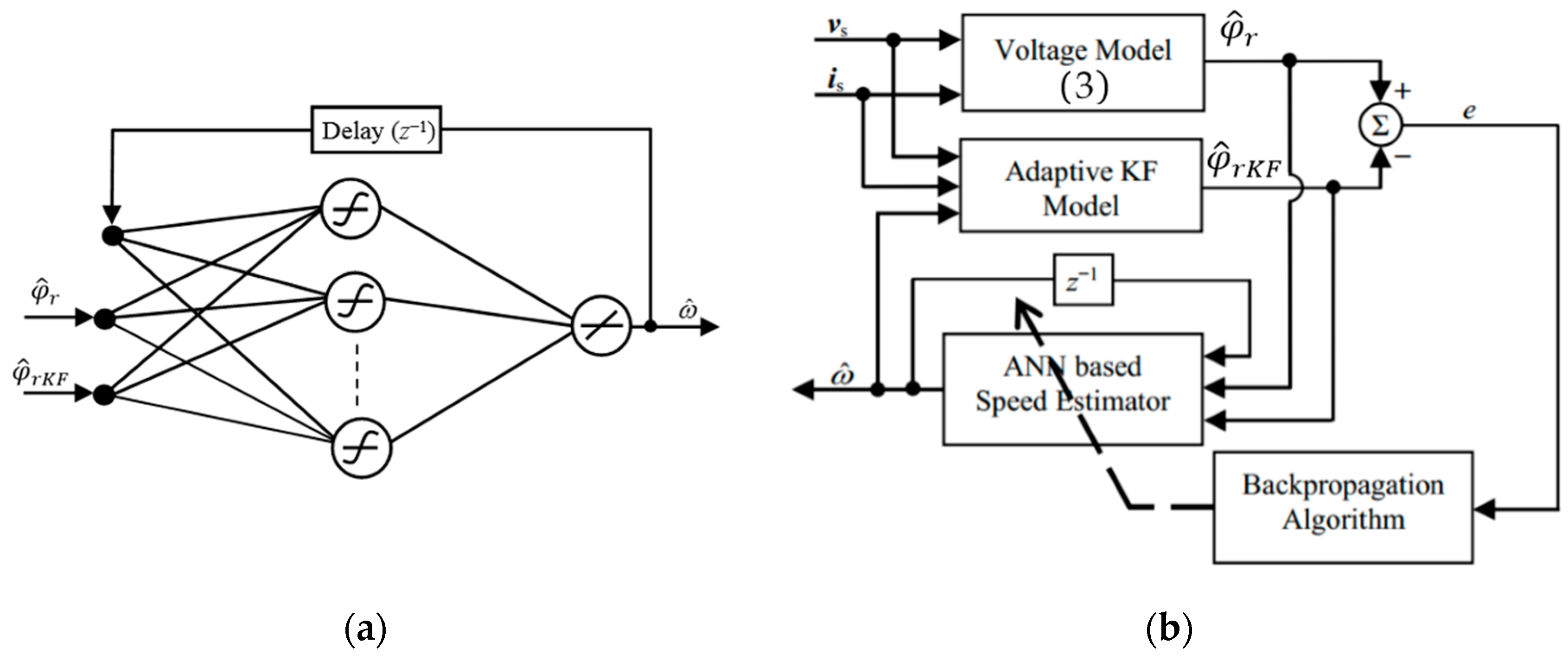
3.3. Artificial Neural Network Speed Estimation

The rotor speed is estimated by the artificial neural network (ANN) shown in Figure 2a. The ANN is a recurrent multilayer network, where the hidden layer is activated by a hyperbolic tangent (tanh) function, and the output layer is activated by a linear function. The ANN output is the estimated rotor speed. The ANN has three inputs:
  • Two external signals (estimated rotor flux from the reference voltage Model (3) and estimated rotor flux from the KF (5)).
  • A feedback from the ANN output with a delay.
The equation of the neuron at the hidden layer and the output are given by
{ h ( k , i ) = t a n h ( w 1 i ω ^ ( k 1 ) + w 2 i φ ^ r ( k ) + w 3 i φ ^ r K F ( k ) ) ω ^ ( k ) = i = 1 N w i h ( k , i )
where, ω ^ is the estimated rotor speed, h is the neuron expression at the hidden layer, w j i ; j = 1 3 are the weights from the input layer to the hidden layer, wi; i = 1 N are the weights from the hidden layer to the output layer, and N is the number of neurons in the hidden layer.
The ANN training is carried out online, using the flux error between the rotor flux ( φ ^ r ) estimated by the reference voltage Model (3) and the rotor flux ( φ ^ r K F ) estimated by the adaptive KF (5), as shown in Figure 2b, to update the ANN weights [30]. The backpropagation algorithm is used for the training process, and the weights are updated using the equations
w i ( k + 1 ) = w i ( k ) + μ · h ( k , i ) · e ( k )
w j i ( k + 1 ) = w j i ( k ) + μ · x j ( k ) ( w i ( k ) · ( 1 h ( k , i ) ) · e ( k ) )
where, x j is the ANN input,   j = 1 3 , i = 1 N, e ( k ) = φ ^ r ( k ) φ ^ r K F ( k ) , and   μ is the learning rate.
The implementation of the ANN training algorithm is provided in the flowchart of Figure 3.

4. Load Side Control
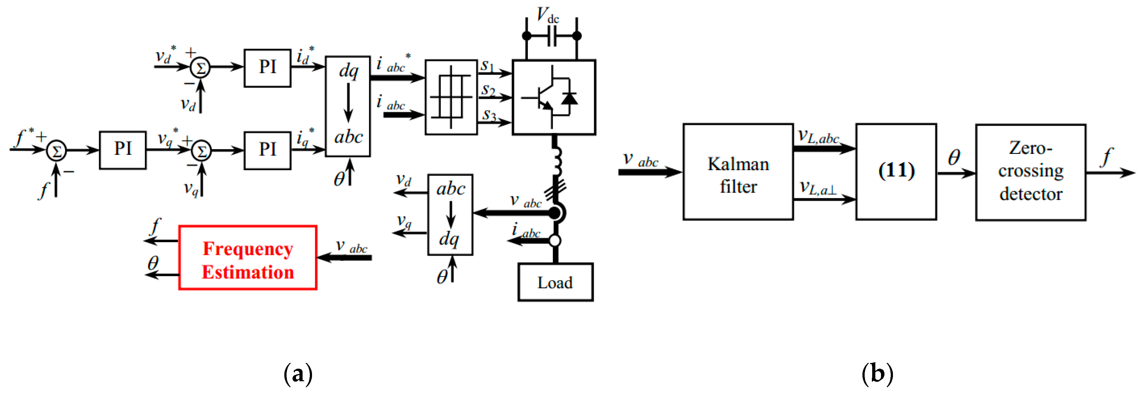
4.1. Control Design

The three-phase AC load is connected to the DC-link through the DC–AC converter (inverter) and a resistive-inductive filter to smoothen the signals. In order to match the voltage and the frequency of the AC load with the system requirements, both quantities are controlled to track specific references. The load side control system includes two control loops in cascade, as depicted in Figure 4a.
The outer control loop regulates the load frequency, to be maintained constant at 60 Hz, and provides the reference for the q-component of the load voltage. The inner control loop has a vector control scheme, based on proportional integral (PI) regulators, to control the direct-quadrature (d-q) components of the load voltage. The three-phase voltages and currents at the load are available by measurements. The d-q components are carried out by the Park transformation. The frequency f and the angular position θ of the (d-q) synchronous rotating reference frame, required in the control system implementation, are available by estimation.

4.2. Frequency Estimation

The implementation of the load side control scheme, shown in Figure 4a, requires information about the frequency. In general, a phase-locked loop (PLL) structure is used for its estimation. The PLL strategy involves the tuning of the voltage control gains to deal with the measurement uncertainties [33,34]. To overcome this issue, an estimation method, based on the Kalman filter, is adopted in this work. It consists of obtaining the fundamental component and an orthogonal component of the three-phase voltages at the load side that is used in the frequency estimation. The advantage of the Kalman filter is the ability to deal with measurement noises through adapting its gains [35,36,37].
The three-phase AC load is considered balanced, and the observed voltages can be expressed as
{ v a ( t ) = V m sin ( ω e t + ϕ ) v b ( t ) = V m sin ( ω e t + ϕ 2 π 3 ) v b ( t ) = V m sin ( ω e t + ϕ + 2 π 3 )
where, Vm is the amplitude, ωe = 2πf is the angular frequency and ϕ is the phase angle.
A discrete state space model of the balanced three-phase sinusoidal system can be generated as follows
{ V L ( k + 1 ) = A · V L ( k ) + w ( k ) v ( k ) = C · V L ( k ) + z ( k )
where,   V L = [ v L a v L b v L c v L a ] T is the state vector of the three-phase filtered voltage signals ( v L a , v L b ,   v L c ) and the orthogonal signal, respective to the phase a, ( v L a ), v = [ v a v b v c ] T is the measured output of the load voltages, w and z are independent noises.
The matrices A and C are given by
A = [ cos ( 2 π N ) 1 3 sin ( 2 π N ) 1 3 sin ( 2 π N ) 0 1 3 sin ( 2 π N ) cos ( 2 π N ) 1 3 sin ( 2 π N ) 0 1 3 sin ( 2 π N ) 1 3 sin ( 2 π N ) cos ( 2 π N ) 0 sin ( 2 π N ) 0 0 cos ( 2 π N ) ] ,   C = [ 1 0 0 0 0 1 0 0 0 0 1 0 ]
where, N = fs/f is the number of samples in the fundamental component and fs is the sampling frequency.
The Kalman filter algorithm, described in Appendix A, is used to estimate the state vector VL using x = VL, y = v, and w and z are independent measurement noises with covariance [37]. Then, the instantaneous phase angle is obtained by
θ ( k ) = tan 1 ( v L a ( k ) v L a ( k ) )
The fundamental frequency f can be estimated from zero-crossing detection of the signal θ(k).
The frequency estimation algorithm is illustrated in Figure 4b. From the load voltage measurements v a b c , the Kalman filter is applied to estimate the voltages ( v a b c ,   v a ). Then, the angle θ is carried out using ( v L a ,   v L a ) as defined in Model (11). Finally, the zero-crossing detection method is used to determine the frequency f.

5. Battery Storage System and Power Management

The wind energy-based microgrid operates in standalone mode by integrating a battery storage system (BSS). The BSS includes a battery bank and a DC-DC buck-boost converter connected to the DC-link, as shown in Figure 5a. The BSS control system regulates the DC-link voltage, to be maintained constant, through the buck-boost converter by charging-discharging the battery bank to meet the load demand. As illustrated in Figure 5a, the bidirectional buck-boost converter is run in continuous conduction mode. The insulated-gate bipolar transistor (IGBT) states s1 and s2 are selected, based on the control system, to operate the converter for charge and discharge modes. The control system includes a PI controller to regulate the DC-link voltage (Vdc) for tracking the voltage reference (Vdc*), and the battery charge-discharge is operated through controlling its current (Ibat) to track a current reference carried out from the powers: Wind generator power (Pw), battery power (PB), and load power (PL); and the battery voltage (Vbat), as shown in Figure 5b.
In this work, it is assumed that the battery bank can store any excess power produced by the wind turbine generator. The charge-discharge process is conducted through a power management system (PMS).
The PMS checks the battery state of charge (SOC) carried out by
SOC = 100 ( 1 +   I bat Q )
where, Ibat is the battery current and Q is the battery capacity.
The constraints on the SOC for the battery storage is given as
SOC min SOC SOC max
where, SOC min   and SOC max are the minimum and the maximum allowable states for safety.
The power management system provides the references to the local controllers (generator and battery) based on the net power (Pnet) and the battery SOC . It follows the flowchart shown in Figure 6.

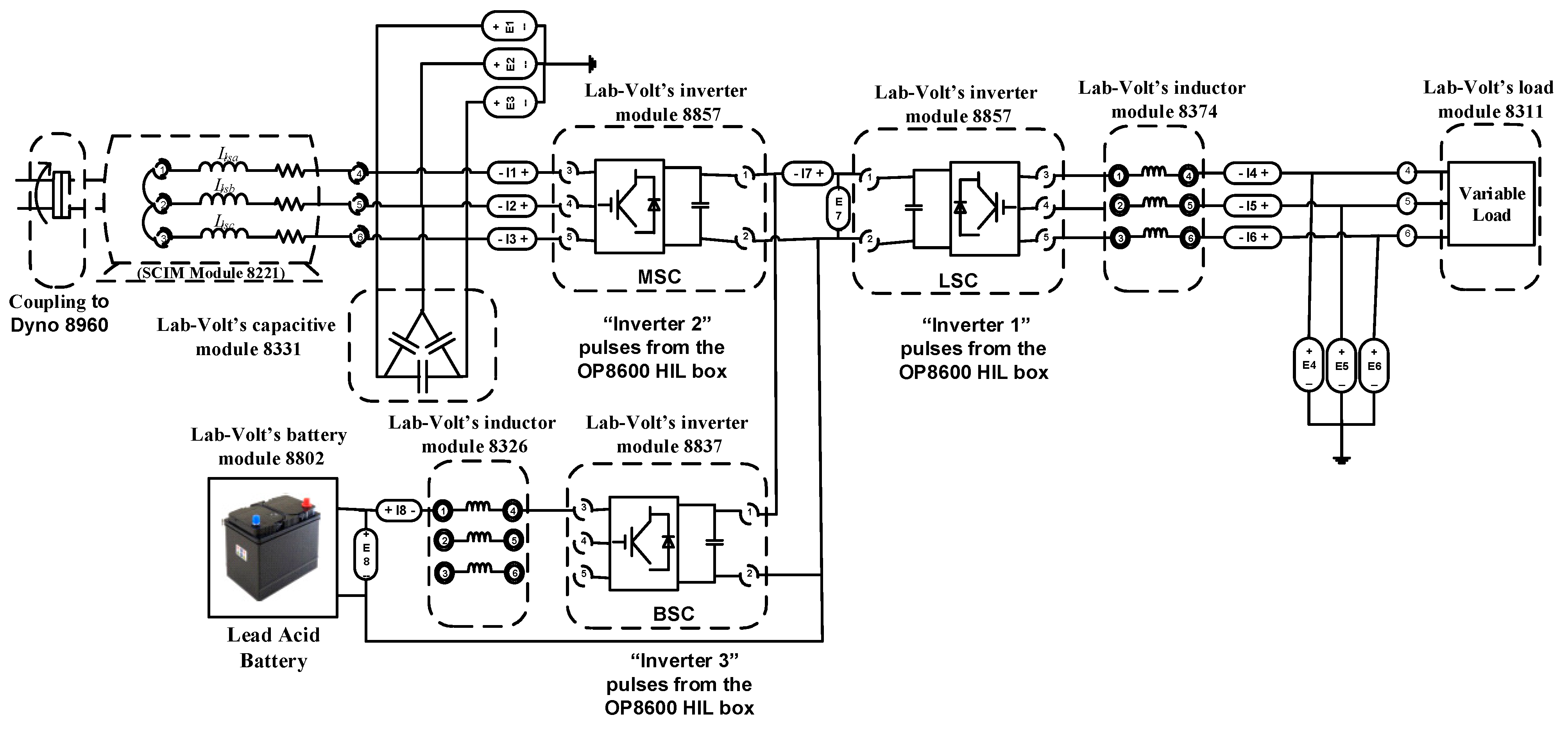
6. Experimental Results

Experiments were conducted using the DC-microgrid experimental setup illustrated in Figure 7. The electric schematic for wiring is shown in Figure 8. The setup includes the following modules:
  • Three-phase squirrel-cage induction generator.
  • Capacitor bank connected to the generator stator terminal for running as a self-started generator.
  • Four-quadrant dynamometer, coupled with the induction generator, for wind turbine emulation.
  • Back-to-back IGBT converters to connect the generator to the load.
  • Bidirectional IGBT DC-DC converter and line inductor to connect the BSS to the DC-link.
  • Battery bank based on lead acid batteries.
  • Three-phase inductor as the filter to connect the DC-AC converter to the load.
  • Variable switching resistor to vary the three-phase AC load.
  • Data acquisition interface (OPAL-RT OP8660) for voltage-current measurements.
  • Real-time digital simulator (OPAL-RT OP5600) for rapid control prototyping and Hardware-in-the-loop (HIL).
The specifications of the squirrel-cage induction machine, the OPAL-RT system, and the other components are available in references [30,34]. The elements’ characteristics are provided in Table 1 and Table 2.
The control and estimation algorithms and the data acquisition were implemented in the MATLAB/Simulink environment and executed in the real-time digital simulator OP5600 through the RT-LAB software, which compiles the Simulink model and runs it in the OP5600 [34]. The control gains were selected by trial and error, to achieve successful performance for the estimation (generator state and load frequency) and the control (rotor speed and DC-link voltage).
The artificial neural network was implemented with N = 6 as the number of neurons in the hidden layer. The sampling time for the ANN and the Kalman filter execution was Ts = 100 μs.
The first experiment was carried out to operate the wind turbine-generator under a variable wind speed profile and a variable load by varying the resistances’ values. Figure 9 presents the responses of the microgrid. The rotor speed estimation and the tracking are shown Figure 9a, where it can be observed that the rotor speed, estimated by the ANN estimation scheme, was well achieved, and the rotor speed was tracking its reference. It can be observed for the speed response in Figure 9a, a zero steady-state error, while a small steady-state error was observed in the speed tracking in reference [24], using the MRAS-sliding mode observer. Furthermore, the speed tracking occurred without an overshoot, compared to the result in reference [15], where a small overshoot was seen at the step transition as the speed estimation depended on the model parameters. In reference [22], the speed response had some oscillations, whereas these fluctuations were not observed in the speed tracking shown in Figure 9a. The power management system operates the charge-discharge of the battery adequately at each change in the load to keep the power balanced in the system, as shown in Figure 9b. The DC-link voltage was successfully regulated, as shown in Figure 9c, despite the step variations in the generator power and the load demand. The battery current, required for such operation, is shown in Figure 9d, and as observed, it follows the variation between the generator power and the load demand. In Figure 10, the d-q components of the load voltage track the voltage references with a good performance, and the frequency was well estimated and regulated to track the reference value despite the variations in the load demand. These results prove the robustness of the proposed estimation-control system to uncertainties due to step variations in the wind speed and the load demand.
In this experiment, the control and the estimation schemes were verified for a random ramp variation of the wind speed by running the dynamometer at a random ramp speed. The estimated rotor speed tracked the dynamometer speed with a good performance, as illustrated in Figure 11a. In this ramp response, it can be observed that a small deviation, between the estimated rotor speed and the reference, was present in a similar way, as in the results of reference [26], which shows a common behavior in the different control methods. The power response was appropriately balanced in order to feed the load with a constant power, as shown in Figure 11b. Again, the DC-link voltage was well regulated, as shown in Figure 11c, despite the speed variation. For the load voltage regulation, a variable profile for the d-component of the load voltage had been used to test the frequency estimation and regulation, as shown in Figure 12a. It can be observed that the d-component of the load voltage tracked the variable reference, and an opposite variable q-component of the load voltage was generated to compensate for the variation of the d-component and maintain the frequency constant, as shown in Figure 12a,b. A closer look at the frequency response, shown in Figure 12b, shows that the frequency is affected by the variation of the d-q components of the load voltage with a fast action of the controller to bring back the frequency to the constant value, which demonstrates the capability of the estimation and control system to overcome the disturbances effect.

7. Conclusions

An estimation strategy, for the rotor speed, the rotor flux and the load frequency, is proposed to implement a vector control scheme on a standalone wind energy DC-microgrid based on induction generator and battery storage. For sensorless operation, the rotor speed is estimated by an ANN-based MRAS method through estimating the rotor flux by a Kalman filter. The adaptive Kalman filter and the artificial neural network, used as estimation models, improve the MRAS scheme due to their online adaptation to deal with parametric variations and uncertainties. At the load side, the frequency is estimated by a Kalman filter to avoid the PLL use due to its drawbacks. The proposed estimation strategy can also be applied for the experimental implementation of other control schemes in wind energy conversion systems based on induction generators.

Author Contributions

Conceptualization, A.A.T. and A.M.; methodology, A.A.T. and A.M.; validation, A.A.T.; formal analysis, A.A.T. and A.M.; writing—original draft preparation, A.A.T.; writing—review and editing, A.M.; supervision, A.M.; project administration, A.M.; funding acquisition, A.M. All authors have read and agreed to the published version of the manuscript.

Funding

This research was funded by CANADA FOUNDATION FOR INNOVATION, grant number 30527.

Conflicts of Interest

The authors declare no conflict of interest.

Appendix A

The time varying Kalman filter algorithm is carried out through the execution of the following steps:
  • State prediction:
x ^ ( k + 1 / k ) = A ( k ) x ^ ( k / k ) + B ( k ) u ( k )
2.
Estimated error covariance:
P ( k + 1 / k ) = A ( k ) P ( k / k ) A T ( k ) + Q
3.
Kalman filter gain calculation:
K ( k + 1 ) = P ( k + 1 / k ) C T ( C P ( k + 1 / k ) C T + R ) 1
4.
State correction:
x ^ ( k + 1 / k + 1 ) = x ^ ( k + 1 / k ) + K ( k + 1 ) ( y ( k + 1 ) C x ^ ( k + 1 / k ) )
5.
Error covariance update:
P ( k + 1 / k + 1 ) = ( I K ( k + 1 ) C ) P ( k + 1 / k )
Initial conditions:
x ^ ( 0 ) = E { x ( 0 ) } ; P ( 0 ) = E { ( x ( 0 ) x ^ ( 0 ) ) ( x ( 0 ) x ^ ( 0 ) ) T }

References

  1. Bansal, R.C. Three-phase self-excited induction generators: An overview. IEEE Trans. Energy Convers. 2005, 20, 292–299. [Google Scholar] [CrossRef]
  2. Chilipi, R.R.; Singh, B.; Murthy, S.S. Performance of a self-excited induction generator with DSTATCOM-DTC drive-based voltage and frequency controller. IEEE Trans. Energy Convers. 2014, 29, 545–557. [Google Scholar] [CrossRef]
  3. Senthil Kumar, S.; Kumaresan, N.; Subbiah, M. Analysis and control of capacitor-excited induction generators connected to a micro-grid through power electronic converters. IET Gener. Transm. Dis. 2015, 9, 911–920. [Google Scholar] [CrossRef]
  4. Gao, S.; Bhuvaneswari, G.; Murthy, S.S.; Kalla, U. Efficient voltage regulation scheme for three-phase self-excited induction generator feeding single-phase load in remote locations. IET Renew. Power Gen. 2014, 8, 100–108. [Google Scholar] [CrossRef]
  5. Singh, B.; Murthy, S.S.; Reddy, R.S.; Arora, P. Implementation of modified current synchronous detection method for voltage control of self-excited induction generator. IET Power Electron. 2015, 8, 1146–1155. [Google Scholar] [CrossRef]
  6. Scherer, L.G.; Tambara, R.V.; De Camargo, R.F. Voltage and frequency regulation of standalone self-excited induction generator for micro-hydro power generation using discrete-time adaptive control. IET Renew. Power Gen. 2016, 10, 531–540. [Google Scholar] [CrossRef]
  7. Urtasun, A.; Barrios, E.L.; Sanchis, P.; Marroyo Palomo, L. Frequency-based energy-management strategy for stand-alone systems with distributed battery storage. IEEE Trans. Power Electron. 2015, 30, 4794–4808. [Google Scholar] [CrossRef]
  8. Korlinchak, C.; Comanescu, M. Sensorless field orientation of an induction motor drive using a time-varying observer. IET Electr. Power Appl. 2012, 6, 353–361. [Google Scholar] [CrossRef]
  9. Merabet, A.; Rajasekaran, V.; McMullin, A.; Ibrahim, H.; Beguenane, R.; Thongam, J.S. Nonlinear model predictive controller with state observer for speed sensorless induction generator–wind turbine systems. Proc. Inst. Mech. Eng. Part I J. Syst. Control Eng. 2013, 227, 198–213. [Google Scholar] [CrossRef]
  10. Zhao, K.; You, X. Speed estimation of induction motor using modified voltage model flux estimation. In Proceedings of the IEEE 6th International Power Electronics and Motion Control Conference, Wuhan, China, 17–20 May 2009; pp. 1979–1982. [Google Scholar]
  11. Bensiali, N.; Etien, E.; Benalia, N. Convergence analysis of back-EMF MRAS observers used in sensorless control of induction motor drives. Math. Comput. Simul. 2015, 115, 12–23. [Google Scholar] [CrossRef]
  12. Orlowska-Kowalska, T.; Dybkowski, M. Stator-current-based MRAS estimator for a wide range speed-sensorless induction-motor drive. IEEE Trans. Ind. Electron. 2010, 57, 1296–1308. [Google Scholar] [CrossRef]
  13. Gadoue, S.M.; Giaouris, D.; Finch, J.W. Stator current model reference adaptive systems speed estimator for regenerating-mode low-speed operation of sensorless induction motor drives. IET Electr. Power Appl. 2013, 7, 597–606. [Google Scholar] [CrossRef] [Green Version]
  14. Marcetic, D.P.; Krcmar, I.R.; Gecic, M.A.; Matić, P.R. Discrete rotor flux and speed estimators for high-speed shaft-sensorless IM drives. IEEE Trans. Ind. Electron. 2014, 61, 3099–3108. [Google Scholar] [CrossRef]
  15. Merabet, A.; Tanvir, A.A.; Beddek, K. Torque and state estimation for real-time implementation of multivariable control in sensorless induction motor drives. IET Electr. Power Appl. 2017, 11, 653–663. [Google Scholar] [CrossRef]
  16. Barut, M. Bi Input-extended Kalman filter based estimation technique for speed-sensorless control of induction motors. Energy Convers. Manag. 2010, 51, 2032–2040. [Google Scholar] [CrossRef]
  17. Mazaheri, A.; Radan, A. Performance evaluation of nonlinear Kalman filtering techniques in low speed brushless DC motors driven sensor-less positioning systems. Control Eng. Pract. 2017, 60, 148–156. [Google Scholar] [CrossRef]
  18. Alonge, F.; D’Ippolito, F.; Sferlazza, A. Sensorless control of induction-motor drive based on robust Kalman filter and adaptive speed estimation. IEEE Trans. Ind. Electron. 2014, 61, 1444–1453. [Google Scholar] [CrossRef]
  19. Habibullah, M.; Lu, D.D.-C. A speed-sensorless FS-PTC of induction motors using extended Kalman filters. IEEE Trans. Ind. Electron. 2015, 62, 6765–6778. [Google Scholar] [CrossRef]
  20. Farasat, M.; Trzynadlowski, A.M.; Fadali, M.S. Efficiency improved sensorless control scheme for electric vehicle induction motors. IET Electr. Syst. Transp. 2014, 4, 122–131. [Google Scholar] [CrossRef]
  21. Zerdali, E.; Barut, M. The comparisons of optimized extended Kalman filters for speed-sensorless control of induction motors. IEEE Trans. Ind. Electron. 2017, 64, 4340–4351. [Google Scholar] [CrossRef]
  22. Cirrincione, M.; Accetta, A.; Pucci, M.; Vitale, G. MRAS speed observer for high-performance linear induction motor drives based on linear neural networks. IEEE Trans. Power Electron. 2013, 28, 123–134. [Google Scholar] [CrossRef]
  23. Al-Ghossini, H.; Locment, F.; Sechilariu, M.; Gagneur, L.; Forgez, C. Adaptive-tuning of extended Kalman filter used for small scale wind generator control. Renew. Energy 2016, 85, 1237–1245. [Google Scholar] [CrossRef]
  24. Ammar, A.; Kheldoun, A.; Metidji, B.; Ameid, T.; Azzoug, Y. Feedback linearization based sensorless direct torque control using stator flux MRAS-sliding mode observer for induction motor drive. ISA Trans. 2020, 98, 382–392. [Google Scholar] [CrossRef] [PubMed]
  25. Korzonek, M.; Tarchala, G.; Orlowska-Kowalska, T. A review on MRAS-type speed estimators for reliable and efficient induction motor drives. ISA Trans. 2019, 93, 1–13. [Google Scholar] [CrossRef]
  26. Pal, A.; Das, S.; Chattopadhyay, A.K. An improved rotor flux space vector based MRAS for field oriented control of induction motor drives. IEEE Trans. Power Electron. 2018, 33, 5131–5141. [Google Scholar] [CrossRef]
  27. Zerdali, E.; Mengüç, E.C. Novel complex-valued stator current-based MRAS estimators with different adaptation mechanisms. IEEE Trans. Instrum. Meas. 2019, 68, 3793–3795. [Google Scholar] [CrossRef]
  28. Velo, R.; López, P.; Maseda, F. Wind speed estimation using multilayer perceptron. Energy Convers. Manag. 2014, 81, 1–9. [Google Scholar] [CrossRef]
  29. Jaramillo-Lopeza, F.; Kenne, G.; Lamnabhi-Lagarrigue, F. A novel online training neural network-based algorithm for wind speed estimation and adaptive control of PMSG wind turbine system for maximum power extraction. Renew. Energy 2016, 86, 38–48. [Google Scholar] [CrossRef]
  30. Merabet, A.; Tanvir, A.A.; Beddek, K. Speed control of sensorless induction generator by artificial neural network in wind energy conversion system. IET Renew. Power Gen. 2016, 10, 1597–1606. [Google Scholar] [CrossRef]
  31. Gadoue, S.M.; Giaouris, D.; Finch, J.W. Sensorless control of induction motor drives at very low and zero speeds using neural network flux observers. IEEE Trans. Ind. Electron. 2009, 56, 3029–3039. [Google Scholar] [CrossRef]
  32. Maiti, S.; Verma, V.; Chakraborty, C.; Hori, Y. An adaptive speed sensorless induction motor drive with artificial neural network for stability enhancement. IEEE Trans. Ind. Inform. 2012, 8, 757–766. [Google Scholar] [CrossRef]
  33. Ciobotaru, M.; Teodorescu, R.; Blaabjerg, F. A new single-phase PLL structure based on second order generalized integrator. In Proceedings of the 37th IEEE Power Electronics Specialists Conference, Jeju, Korea, 18–22 June 2006; pp. 1–6. [Google Scholar]
  34. Merabet, A.; Ahmed, K.T.; Ibrahim, H.; Beguenane, R.; Ghias, A.M. Energy management and control system for laboratory scale microgrid based wind-PV-battery. IEEE Trans. Sustain. Energy 2017, 8, 145–154. [Google Scholar] [CrossRef]
  35. Liu, Y.; Yan, D.; Zheng, H. Signal frequency estimation based on Kalman filtering method. In Proceedings of the 8th International Conference on Computer and Automation Engineering, Melbourne, Australia, 3–4 March 2016; pp. 1–6. [Google Scholar]
  36. Cardoso, R.; Camargo, R.F.D.; Pinheiro, H.; Gründling, H. Kalman filter based synchronisation methods. IET Gener. Transm. Dis. 2008, 2, 542–555. [Google Scholar] [CrossRef]
  37. Marafão, F.P.; Colón, D.; De Padua, M.S.; Deckmann, S.M. Kalman filter on power electronics and power systems applications. In Kalman Filter: Recent Advances and Applications; Moreno, V.M., Pigazo, A., Eds.; IntechOpen: London, UK, 2009; pp. 397–420. [Google Scholar]
Figure 1. Wind energy conversion system: (a) DC-microgrid based standalone self-excited induction generator with battery storage; (b) generator side converter control scheme.
Energies 13 01743 g001
Figure 2. ANN based speed estimation: (a) ANN structure; (b) estimation and ANN training scheme.
Energies 13 01743 g002
Figure 3. Backpropagation training algorithm.
Energies 13 01743 g003
Figure 4. Load side control and estimation: (a) Control scheme; (b) frequency estimation.
Energies 13 01743 g004
Figure 5. Battery storage system: (a) Charge-discharge operation; (b) control system.
Energies 13 01743 g005
Figure 6. Flowchart of the power management system.
Energies 13 01743 g006
Figure 7. Experimental setup.
Energies 13 01743 g007
Figure 8. Connection schematic of the experimental setup.
Energies 13 01743 g008
Figure 9. Control and estimation responses under variable step wind speed profile and variable load: (a) Speed estimation and tracking; (b) power responses; (c) DC-link voltage regulation; (d) battery current.
Energies 13 01743 g009
Figure 10. Load voltage regulation and frequency estimation.
Energies 13 01743 g010
Figure 11. Control and estimation responses under random ramp wind speed profile and constant load: (a) Speed estimation and tracking; (b) power responses; (c) DC-link voltage regulation.
Energies 13 01743 g011aEnergies 13 01743 g011b
Figure 12. Load side control: (a) Controlled d-q load voltages, (b) Frequency control and estimation.
Energies 13 01743 g012
Table 1. Characteristics of the microgrid elements.
ElementCharacteristics
DynamometerFour-quadrant, 0−3 Nm, 0−2500 rpm, 350 W
SCIGFour-pole, 3 phases, 60 Hz, 208 V, 1670 rpm, 175 W
BatteryLead acid, 48 V, 9 Ah, max charge current 2.7
Table 2. Characteristics of the converters and the excitation capacitor bank.
CharacteristicsValues
IGBT power converters
DC-link voltage220 V
IGBT peak current12 A
Switching control (voltage, frequency)0/5 V, 0−20 kHz
Excitation capacitor bank
Power, voltage252 VAR, 120 V
Capacitance8.8 μF
Resistance300 Ω

