Abstract
Theoretical modeling and the sliding mode control (SMC) of an active trailing-edge flap of a wind turbine blade based on the adaptive reaching law are investigated. The blade is a single-celled thin-walled composite structure using circumferentially asymmetric stiffness (CAS) design, exhibiting displacements of flap-wise/twist coupling. A reduced structural model originated from the variation method is used to model the structure of the blade, the structural damping of which is computed. The trailing-edge flap is a rigid structure that is embedded in and hinged to the blade host structure, and it is driven by two pairs of pneumatic cylinders moving in reverse. Flutter suppression for the large-amplitude vibration of the blade tip is investigated based on an active trailing-edge flap structure and SMC algorithm using the adaptive reaching law. The controlled responses of flap-wise/twist displacements and control inputs (the angles of the trailing-edge flap) are illustrated, with obvious simulation effects demonstrated. An experimental platform for driving the pneumatic cylinders verifies the effectiveness of the control algorithm using the adaptive reaching law and the effectiveness of the selected pneumatic transmission scheme controlled by another adaptive SMC based on the minimum parameter learning of neural networks.
1. Introduction
Wind turbine blades have always been involved in large-amplitude vibration in the actuation of unsteady flow states. The large-amplitude vibration of displacements of flap-wise/twist coupling is an important reason for the fatigue damage of blades. In view of the extensive application of composite materials in the construction of blade structures, how to effectively model composite structures for blades of flap-wise/twist coupling and re-strain large amplitude vibration has been a subject to be further studied.
So far, many thin-walled composite structures have been used for the vibration control of rotating blades or beams. In early studies, a refined theory of rotary blades, whose model was a thin-walled composite beam with an arbitrary closed section that contained some nonclassical features, such as the anisotropy and heterogeneity of the constituent materials, transverse shear, and primary and secondary warping, was investigated to study free vibration behavior [1]. The forced vibration of rotating pre-twisted blades modeled as laminated composite hollow uniform box-beams, including transverse shear flexibility, restrained warping, and centrifugal and Coriolis effects, has been presented to analyze the vibration effects [2]. A reduced-order model has been investigated for aeroelastic analysis using the computational fluid dynamics (CFD) codes named CFL3D, in which the state-space expression of unsteady aerodynamic forces was combined with a state-space model of the structure to simulate the aeroelasticity using MATLAB (R2011b, MathWorks, Natick, MA, USA) codes [3]. Various actuators have also been used as control means to achieve flutter suppression. A general method for vibration control of a nonlinear rotary beam using an integral sliding mode control (SMC) approach has been developed. The structural model was modeled as a rotary Euler–Bernoulli beam (EBB) integrated with a piezoelectric actuator [4]. In addition, the structural modeling of rotary pre-twisted thin-walled composite beams, with macro fiber composite actuators and embedded sensors, has been investigated to study vibration analysis and optimal control using higher shear deformation theory [5].
In the last 10 years, various nonlinear theories of composite structure have been successfully used in vibration analysis and aeroelastic control for beams or blades, and various optimization approaches using the finite element model (FEM) or various optimization criteria have been used in structural enhancement or active control to achieve the purpose of improving the aeroelastic behavior of blades. The vibration analysis of a rotary composite structure using assumptions of Timoshenko beam theory and exhibiting nonlinear von-Karman strain–displacement relationships has been investigated, with the three-coupled partial differential equation of vibration motion obtained [6]. Aeroelastic stability analysis of a full-scale composite blade has been investigated, with the aerodynamic loading determined using modified Blade Element Momentum (BEM) theory and CFD method. Then, a 3D FEM was built using the iterative approach of fluid–structure interaction (FSI) to investigate the aeroelastic behavior [7]. After linearizing the nonlinear equations of the wind turbine blades, the active control of the optimal proportional–integral–derivative (PID) control method and the optimized linear quadratic regulator (LQR) are proposed to suppress the flap-wise and lead-lag flutter. [8]. A novel method for the optimization of the blade was developed to eliminate the requirement of stream-tube theory iterations, the criterion of which is maximization of the lift-to-drag ratio [9].
As for the FSI models, some new FSI models have been investigated in recent years. For instance, the structural trailing edge modeling method and trailing-edge flow control have been developed and studied by different scholars to enhance the reliability of the structural performance for blades. Haselbach proposed an advanced structural modeling method based on a shell element model where the adhesive bond-line in the trailing edge region was discretized by solid brick elements, which enhance the reliability of structural predictions for blades [10]. Llorente and Ragni presented an experimental study focusing on the change of the aerodynamic performance of blades with the employment of trailing-edge serrations, and they discussed the procedure design and prediction methodology [11]. Qin and Chen reported an investigation into the performance of trailing-edge flow control devices, including microtabs and microjets installed (near the trailing edge) by solving the three-dimensional Reynolds averaged Navier–Stokes equations (NSE) [12]. Huang et al. used the trailing-edge flap and mid-span flap (deflected in opposite directions such that the root bending moment of the blade remains almost unchanged) to excite the unstable modes of the tip vortex system of blades to investigate the mechanism of how and to what extent the deflection of the flaps influences the tip vortex system [13]. Thakur et al. investigated the load mitigation effects using blade trailing-edge flaps subjected to turbulent wind, with the BEM theory used to obtain the aerodynamic loads by modeling in a multi-body framework while the hydrodynamic and geotechnical analysis were performed in a FEM framework [14]. Another trailing-edge-based literature, in which the modeling of an aeroelastic system of a blade section based on a trailing-edge flap using a new proposed aerodynamics model has been investigated, demonstrated vibration analysis of the blade section exhibiting flap-wise/twist displacements and performed flutter suppression by equivalent SMC [15].
In addition, other flap structures have also been used by different scholars to reduce the loads of the blades and enhance the aerodynamic performance. For example, a gurney flap (GF) placed at the pressure side of the trailing edge of an airfoil and perpendicular to the chord line can enhance lift in wind turbine blades and enhance the aerodynamic performance of airfoils, making it generate more lift and delaying the onset of stall [16,17,18]. Bianchini presented numerical analysis using CFD with the aim of evaluating the potential of using GFs for the power augmentation of Darrieus turbines [16]. Zhang et al. presented a computational investigation on the effects of two configurations of GFs on the aerodynamic performance with the computational method applied in the investigation solving the Reynold-averaged NSE with a multiple reference frame approach, which models the rotating turbulent flow over the rotor [17].
As everyone knows, strong winds severely endanger the structural integrity of wind turbines, especially when extreme winds are raging. A particular focus of high-amplitude vibration was placed on the effect of strong wind speed and a large change of wind direction on tower collapse and blade fracture [19]. The application of a morphed trailing-edge flap can significantly reduce the excessive loads that cause the damage of blades and surrounding components in wind turbines, and reduce the vibration amplitude of the blade tip [20]. Meanwhile, the adaptive trailing-edge flap control has been proven to be able to play a continuous optimized motion process during the aircraft continuous operation, where the adaptive process was implemented by a Shape Memory Alloy rotary actuator that integrated into the hinge line of a small flap on the trailing edge [21].
In the present study, the theoretical modeling and SMC of an active trailing-edge flap of a composite blade based on the adaptive reaching law are investigated. The blade is a single-celled thin-walled composite structure using CAS configuration, exhibiting displacements of flap-wise/twist coupling. To study the structural modeling and vibration control of CAS-based composite blades, the following two aspects can be considered. The first aspect focuses on precise structural modeling; hence, structural nonlinear and geometrically nonlinear might be considered in theoretical modeling as well, due to the completeness of the structural model. Second, focusing on accurate aerodynamic analysis, the accuracy and completeness of the aerodynamic data obtained are of great significance to the analysis of the dynamic behavior of wind turbine blades, since the aerodynamic characteristics of an airfoil along the spanwise direction are the basis of the aerodynamic performance design of a blade. For instance, an excellent nonlinear beam theory using the weak-form quadrature element method [22] was proposed for the analysis of composite blades. The theoretical novelty was characterized by extending EBB theory to a generalized Timoshenko beam. Meanwhile, mechanics-based variables were used to describe finite rotation [22]. In view of this, in the present study, an alternative scheme for structural modeling and a novel and accurate description of aerodynamics are applied to the blade. The main contributions can be outlined as: (a) A refined variation method model is used to model the structure of a composite blade, integrated with structural damping, which has been is rarely studied. (b) The active trailing-edge flap that is used is a rigid structure instead of a conventional flexible structure, with a novel aerodynamic model acting on the cross-section of an airfoil. (c) The active trailing-edge flap is driven by pneumatic cylinders using a pneumatic transmission scheme instead of conventional mechanical or hydraulic driving excitation. (d) The adaptive SMC algorithm used for stability control is based on the adaptive reaching law, the control inputs of which are ladder signals that can exactly match the performance requirements of pneumatic cylinders driven by pneumatic transmission. (e) An adaptive SMC algorithm based on the minimum parameter learning of neural networks is investigated to control the pneumatic transmission system so as to accurately drive the action of the active trailing-edge flap structure. (f) Owing to the large wind power system being mostly controlled by Programmable Logic Controller (PLC), some intelligent control algorithms cannot be implemented in PLC hardware because of their complexity. The purpose of the experimental platform in the present study is to verify the feasibility of the theoretical control algorithms that can run perfectly in the actual PLC control hardware.
2. Aeroelastic Equations
2.1. Equations of Motions
Figure 1 shows the CAS-based blade system with the rigid trailing-edged flap structure. Figure 1a shows the single-cell thin-walled blade system and the displacements; Figure 1b shows the actual cross-section in position l1, with the middle-line equation (the green dotted line) of the section fitted in terms of NACA 6315 profile and expressed as specific equations [23]; Figure 1c shows the equivalent cross-section with parameters at position l1.
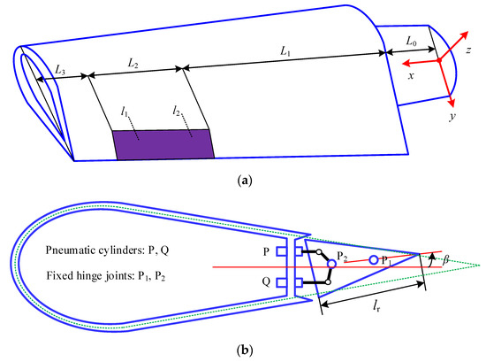
Figure 1.
The circumferentially asymmetric stiffness (CAS)-based blade system with the rigid trailing-edged flap: (a) The CAS-based blade system with the trailing-edged flap; (b) The actual cross-section at position l1; (c) The equivalent cross-section with parameters in position l1.
In Figure 1a, the blade length is m, with the wedge length being m. The length of the rigid trailing-edged flap is L/4, which is located in the center of the anterior half of the blade span (near the tip of the leaf). The displacements are denoted by flap-wise bending (perpendicular to the rotating plane) and twist angle .
In Figure 1b, P and Q are two pneumatic cylinders located in position l1 in Figure 1a. Two piston rods of the two cylinders are connected to the fixed joint P2 (in the rigid trailing-edged flap) through two connecting rods. P1 is another hinge point, which is connected to the host structure of the blade through a shaft. The position point P1 is above the midline of the blade section with slight deviation so that the swing angle of trailing-edge flap is within the range of –15 to 18 degrees. When the two piston rods synchronously move, in reverse, the trailing-edge flap structure can deflect. Note that the other two cylinders with the same function are installed in position l2.
The structural parameters of the equivalent section of blade in Figure 1c are as follows: the wind inflow angle is ψ decided by wind velocity U = 10 m/s, rotating speed Ω, and sectional position. The aerodynamic forces consist of Lift F and Moment M. The rotor rotating speed is Ω = λU/(L + L0), where the tip speed ratio λ = 1. The variable chord length c can be fitted as the form of Fourier Series Models according to an optimization design for the blade [24]. The composite properties are as follows: the sectional thickness is h; the ply thickness is 6.35 × 10⁻⁴ m; the ply angle is denoted by θp; the sectional element mass is mb decided by density ρb = 1672 kg/m3; and the other elastic parameters are marked as G12 = 3.5GPa, E1 = 24.8 GPa, E2 = 8.7 Gpa, and v12 = 0.34.
The circumferentially asymmetric stiffness (CAS) figuration of the composite structure is designed by two assumptions: (a) The spanwise stiffness is far greater than those of vertical/twist directions; the effect of the axial inertia term is much smaller than others and can be ignored. (b) The CAS ply-angle distribution uses the ply-angle law [θp]6 in the top (above the chord and perpendicular to the chordwise direction) flange and [–θp]6 in the bottom flange.
As mentioned above, the structural nonlinear and geometrically nonlinear might be considered in theoretical modeling as well due to the completeness of the structural model. However, in our previous work, we found that after the linear modeling is integrated with composite structural damping, its vibration characteristics, such as fundamental frequencies, are very close to those of the actual composite structure in experiment; that is to say, it can also be equivalent as another complete description of the composite structural model. Hence, in the present study, a refined thin-walled beam theory focused on the CAS situation and subjected to bending–twist coupling is investigated and integrated with structural damping [23,25]. Consider the reduced CAS-based configuration in Reference [26], the independent bending–twist coupling displacement equations are displayed based on a composite cantilever structure. Therefore, after considering the dynamic rigidity effects caused by rotation, the equations of motions of the rotating blade section can be approximatively expressed as follows:
where parameters are the stiffness coefficients that are composed of reduced axial stiffness A(s), coupling stiffness B(s), and shear stiffness C(s), respectively, which can be found in Reference [26]. The other parameters are depicted as:
and the aerodynamic force and moment on the right-side of Equations (1) and (2) can be written as follows [15]:
where is the controlled angle of the trailing-edge flap; and the related aerodynamic coefficients are as follows: , , .
It should be stated that the expressions of aerodynamic force and moment are a novel set of quasi-steady-state hydrodynamic equations, which are suitable for the analysis of the rigid trailing-edge flap behavior of the rotating blade. In particular, for the length lr of the trailing-edge flap in the spanwise direction, it is exactly a specified value lr = c/6. In addition, the expressions of Lift and Moment in Equations (3) and (4) are only used for the aerodynamic calculation of the trailing-edge flap structure, while the Beddoes–Leishman model based on fitted aerodynamic coefficients [23] is used to calculate the stall-induced aerodynamics of the other structural parts along the spanwise direction in this study.
To solve Equations (1)–(4), modal approximation based on Galerkin approach [23] is applied. It might be assumed that:
where and are the N × 1 mode vectors (N = 5 is considered sufficient to meet the accuracy requirements of the series in the present study); and are the 1 × N vectors of the shape functions, respectively.
Substitute Equations (5), (6) into Equations (1)–(4) with the Galerkin method applied, and assume , in the integral process of the Galerkin method along the direction of blade extension, the integral and sum of the three lengths of , and are performed respectively. It results in:
where , and are matrices, and is the matrix.
2.2. Calculation of Structural Damping
By removing the aerodynamics and rotation effects from Equations (1) and (2), only the free vibration equations (FVE) of cantilever structure are considered. To investigate the vibration of the slender cantilever blade, a method using the modal damping ratio and sectional stiffness matrix FVE is deduced to compute the structural damping [23]. Structural damping matrix , which originated from the structural parts of the free vibration equations of the cantilever section in Equations (1) and (2), can be depicted as:
where and are the first-order natural frequency and modal damping ratio. For subsequent research, we define as the corresponding modal damping factor. Note that structural damping is a characteristic of the structure itself, so Equation (8) does not contain rotational effects.
The modal damping ratio in Equation (8) can be defined as the ratio of dissipation (damping) energy and maximum strain energy in each vibration period [27]:
where is the modal vector, and matrices and are the equivalent damping matrix and stiffness matrix. Herein, and satisfy the characteristic equation of the composite thin-wall beam:
where and are the matrices and in Equation (7), from which the rotation effect and the hydrodynamic effect are eliminated. Herein, is a natural frequency. The expression of is the same as , but the terms A(s), B(s), and C(s) in must be replaced by similar parameter terms Ad(s), Bd(s), and Cd(s) in , respectively [25].
The modal damping factors (as) versus ply angles, ranging from 0° to 90°, are displayed in Figure 2.
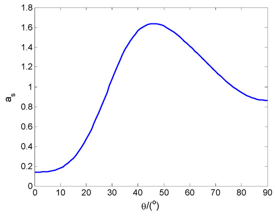
Figure 2.
Damping parameter factors (as) vs. ply angles.
Integrate Cs into Equation (7) and implement the indicated integration in the Galerkin method, resulting in the matrix equations of motions:
where
.
3. Vibration Control based on Adaptive SMC
To continue the subsequent implementation, transform Equation (11) into the state-space expression:
where
.
To carry on furthermore solving by discrete SMC, Equation (12) can be transformed into the discrete state-space as follows:
In recent years, SMC approaches integrated with the Lyapunov method [28,29] have been successfully used in position control for high-performance real-time applications of rotary machines. A more refined discrete equivalent SMC algorithm was used to realize vibration control by adjusting the angle of the trailing-edge flap [15], whereas the angle adjusting was treated as a theoretical time-dependent external input. In the present study, vibration control of the aeroelastic system Equation (13) using SMC has potentially ruled out the physical effect of the entity system that performed external control; otherwise, the external entity system will affect the equations of the structural model in Equations (1) and (2). Hence, the actual driving of the trailing-edge flap here is preferably also a time-independent process using a practical time-dependent external input.
However, for the physical driving system of the trailing-edge flap, the driving based on a mechanical structure system (MST) or hydraulic transmission system (HTS) is bound to directly affect the modeling of the structure. At the same time, as the mathematical model of MST or HTS of the high-order system itself, it should also be introduced into the aeroelastic system of Equation (11), which greatly increases the complexity of system analysis and control. Therefore, in the present study, a pneumatic transmission instead of hydraulic transmission or mechanical process is introduced into the control process of the trailing-edge flap. Since the pneumatic transmission system is installed in the hub and the weight of the connecting parts is almost negligible, the pneumatic transmission itself does not affect the structural modeling of the blade, and it is really a time-independent process.
Pneumatic transmission is fast and its impact is exactly suitable for the angle control of a trailing-edge flap, which requires the control input of the SMC algorithm to have the characteristics of a ladder signal or step signal. Many SMC algorithms can effectively alleviate the chattering phenomenon and suppress the instable vibration. However, there are very few discrete SMC algorithms that not only satisfy the control effect but also have the control inputs similar to ladder signals. The SMC based on the adaptive reaching law is one of these algorithms [30]. It is based on an improvement discrete exponential reaching law. The sliding mode variable structure control law of the discrete system is designed by using the original discrete reaching law, which has many advantages, but due to the influence of the parameters of discrete reaching and the sampling period of the discrete time system, the system will have great chattering.
3.1. Theory of Discrete Exponential Reaching Law
The original discrete exponential reaching law is as follows [30]:
where is the sliding mode function; the sampling time , and for , each is an empirical positive parameter. Then, Equation (14) can be deduced as:
For Equation (14), the following three cases are analyzed:
- when , we can obtainthen, if , we can obtain , and it is a decreasing sequence.
- when , we can obtainthen, if , we can obtain , and it is an incremental sequence.
- when , we can obtainthen, if , we can obtain , and it is in an oscillatory state.
It can be seen from the above analysis that the necessary and sufficient condition for decreasing is
Hence, when , the steady-state oscillatory amplitude of sliding mode motion is as follows
3.2. Theory of SMC based on Adaptive Reaching Law (SMC/ARL)
In the discrete approach law shown in Equation (14), the parameter plays a very important role. The value is small, which can reduce the buffeting of the system. However, if the value is too small, it will affect the approaching speed of the system to the switching surface. At the same time, due to technical factors, the sampling period cannot be very small. Therefore, the ideal value should be time-varying; that is, the value should be larger at the beginning of the system motion, and it should decrease gradually with the increase of time.
It can be seen from Equation (16) that only by making , will decrease, which requires ; that is, should satisfy:
Let us assume , if satisfies , then Equation (18) can be confirmed and satisfied.
Considering Equation (14) and Equation (18), an improved adaptive reaching law can be obtained:
Assuming that the ideal values of the controlled displacements and their first derivatives are zeros (i.e., the position command and speed command of the blade tip are both zeros), the corresponding sliding mode function can be defined as ; then, for discrete system Equation (13), the related control law can be described as:
where the adjustment matrix is deduced in the form of a quadratic-feedback-based matrix as follows.
To facilitate the realization of adaptive computation, a quadratic-feedback method is used to obtain the adjustment matrix Ce. The system Equation (13) can be transformed as:
where . The adjustment matrix is the feedback controller in LQR design, and satisfies Hurwitz stability.
Firstly, suppose that the Lyapunov function V and mode function are as follows
Then, there exists:
Due to the existence of a certain moment , satisfy ; then, , and then
To ensure that , we should prove that .
Due to the linear matrix inequality design [27], when is a symmetric positive definite matrix, we can obtain:
where the weighting coefficient is designed in the LQR controller.
The stability analysis of the sliding mode approach law shown in Equation (16) is as follows:
The sliding mode approach law shown in Equation (19) satisfies the conditions of existence and arrival of discrete sliding modes; hence, the designed control system is stable.
4. Analysis and Discussion
The related parameter values of the large-amplitude vibration of the blade system, including the structural parameters and external motion parameters, follow the values given in Section 2. Figure 3 shows the uncontrolled twist /flap-wise displacements under conditions of ply angles , respectively. With respect to the distance m from the blade tip to the hub, when , the twist displacement exceeds 1.6 rad, which is merely a theoretical simulation, and this is not possible in practice, since the twist displacement may lead to a failure of the blade when the value of twist displacement is up to 1.6 rad. Furthermore, the flap-wise displacements in the cases of various ply angles are more than 2.5 m, which is also impossible relative to the total length of blade, and it may also directly lead to the failure of the blade in practice. The following control algorithms and processes in the present study are designed to solve this kind of large-amplitude vibration problem. Due to the physical limitations of the trailing-edge flap structure, the twist displacements of the blade itself cannot be too large, so this requires that we should select a larger layer angle as the actual ply angle of the blade, since the twist displacements exhibit a linearly decreasing state as the layer angles increase (see Figure 3). However, because the excessive ply angle will inevitably lead to the increase of the lead-lag displacement in the direction (due to the physical orthogonality of the direction and the direction), the influence of the lead-lag displacement coupling cannot be ignored; hence, in this study, the cases of are especially taken for study.
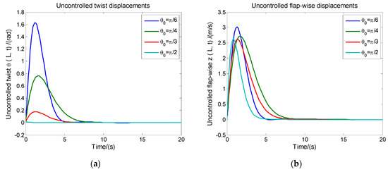
Figure 3.
The uncontrolled twist/flap-wise displacements under conditions of ply angles , respectively: (a) The uncontrolled twist displacement; (b) The uncontrolled flap-wise displacement.
To realize the simulation, the situational parameters are as follows. The initial conditions are ; the sampling time s; the simulation Solver is ODE45, and the desired position signals are , which is a 20-element zero vector. The controller parameters are .
4.1. The Controlled Displacements and Control Signals
Figure 4a shows the controlled twist /flap-wise displacements under conditions of ply angles with , respectively. The SMC/ARL algorithm is very effective in vibration amplitude control. Even at a large wind speed , the displacement fluctuations for both the twist direction and flap-wise direction are within an acceptable range. Compared with the amplitudes in Figure 3, those are greatly suppressed. Figure 4b shows the control inputs (trailing-edge flap angles ) and sliding mode functions (s). The range of the control input signals is within , which is exactly consistent with the limited range of the physical pendulum angles mentioned above. The control input signals are exactly the ladder signals mentioned above, which are not only a performance embodiment of the adaptive reaching law, but they are also suitable for the control requirements of the subsequent pneumatic transmission of the air cylinders. Figure 4b also shows the related sliding mode functions which fluctuate smoothly within a moderate range. The sliding mode functions are accompanied by the steady-state oscillatory amplitudes (denoted by blue lines, which are also within reasonable ranges of fluctuations) of sliding mode motions.
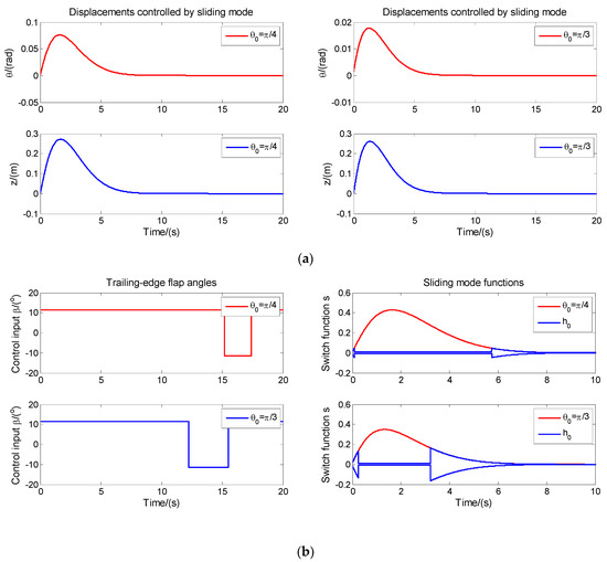
Figure 4.
The controlled displacements and control signals: (a) The controlled displacements under conditions of ply angles with , respectively; (b) The control inputs (trailing-edge flap angles) and sliding mode functions.
4.2. Pneumatic Transmission System
The pneumatic transmission system to drive the two pneumatic cylinders, located in position of l1 in Figure 1a, is mainly composed of a gas source processing unit, two proportional valves, a set of pneumatic pipeline systems, a four-bar linkage mechanism, and two pneumatic pressure cylinders. Please refer to the experiment section in the present study. It can be modeled as a fifth-order transfer function [31]; then, the Optimal Hankel Norm [32] is used to make a model reduction, so a reduced second-order model can be obtained, and with the Laplace Inverse Transform applied, the equation of the pneumatic driving behavior can be deduced as:
where is the current intensity to control the pneumatic proportional valve.
4.2.1. Adaptive SMC based on Minimum Parameter Learning of Neural Networks
For a long time, fuzzy control and neural network control have played an important role in the process optimization [33] and parameter optimization [34] of a rotating mechanical system. To make the change of track the control input signal of the SMC/ARL algorithm displayed in Figure 4b, another algorithm of adaptive SMC based on the minimum parameter learning of neural networks (ASMC/MPLNN) is investegated. It uses parameter estimation instead of neural network weight adjustment, and the adaptive algorithm is simple and convenient for practical engineering application.
Rewrite the Equation (25) as:
The location instruction is exactly the control input signal displayed in Figure 4b. The error signal is . The switching function in the SMC algorithm, whihc is composed of and controller parameter , is expressed as:
where , then
Since in Equation (28) is uncertain, it is impossible to design the control law directly, and it needs to be estimated approximately. Adaptive SMC control based on an Radial Basic Function (RBF) network approximation can be expressed as follows:
where is the input signal of the network; is the number of nodes in the hidden layer of the network; is the output of the Gaussian basis function; is an ideal weight; and is the approximate error of the neural network.
According to the expression of , the input signal is designed as ; then, the output of the RBF network is [30]
To realize minimum parameter learning, one might design as well. If is an estimate of , then . The control law can be devised as:
where the learning rate and the controller parameter .
Define the Lyapunov function as:
where the positive adaptive parameter , then
Assume the adaptive law is:
where , then
Let satisfy , then
where , then solving inequality in Equation (36), it can be obtained:
then
In this design, there is no need for a complex training process in the minimum parameter learning of neural networks. In the derivation of Equations (32) to (38), we have adopted the following two conclusions:
(1)
(2) Since , then , i.e., .
It converts the neural network weight into the unit parameter and accelerates the solution of the adaptive law shown in Equation (34). This is exactly what the minimal parameter learning means. Since the upper bound of the neural network weight is used as its estimate value and the inequality is used to enlarge it, it is a conservative but fast algorithm.
Figure 5 shows the real-time tracking of trailing-edge flap angles and the real-time diaplacements controlled by pneumatic cylinders under conditions of , respectively. The real-time values of the trailing-edge flap angles (denoted by red lines in Figure 5a) are the driving results of the pneumatic transmission system based on the ASMC/MPLNN algorithm. The theoretical values of the trailing-edge flap angles are denoted by blue dot lines, which are exactly the results in Figure 4b. From the tracking results of real-time values to theoretical values, it can be seen that the motions of the pneumatic cylinders can match the change of angles perfectly, and only small overshoots occur where the changes of ladder functions occur.
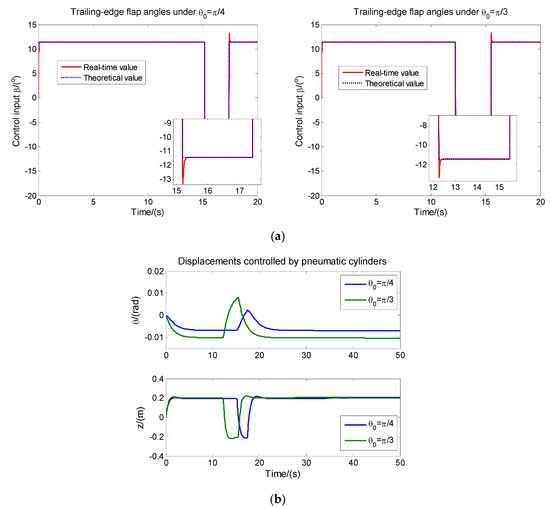
Figure 5.
The real-time tracking of trailing-edge flap angles and the real-time diaplacements controlled by pneumatic cylinders under conditions of , respectively: (a) The real-time tracking of trailing-edge flap angles; (b) The real-time diaplacements controlled by pneumatic cylinders.
Figure 5 also shows the real-time diaplacements controlled by pneumatic cylinders under conditions of , respectively. Compared with the theoretical diaplacements controlled by the SMC/ARL algorithm in Figure 4a, the twist () amplitudes of the real-time controlled diaplacements in Figure 5b reflect almost the same amplitude of theoretical diaplacements, which shows a good real-time control effect. The flap-wise () amplitudes of the real-time controlled diaplacements are almost twice those of the theoretical diaplacements, which demostrates that the real-time control effect is somewhat inferior to the theoretical control. However, compared with the uncontrolled effect in Figure 3, it still embodies the reasonable control effect, which in turn confirms the effectiveness of the theoretical control algorithms. In addition, compared with the theoretical diaplacements controlled in Figure 4a, the fluctuations of the real-time displacements in Figure 5b have great sudden changes within the time range of , which are probably caused by the overshoots produced in the process of angle tracking in Figure 5a. However, the displacement amplitude of this kind of large sudden fluctuation still does not exceed the fluctuation range of the displacement amplitude under theoretical control in Figure 4a, which further confirms that the maximum overshoot in the process of angle tracking is reasonable, thus verifying the effectiveness of the ASMC/MPLNN algorithm.
It should be stated that the comparison case here is not a performance comparison between two sliding-mode algorithms. The two sliding mode algorithms deal with different objects separately. The first sliding mode algorithm SMC/ARL, which was used to solve the aeroelastic system shown in Equation (13), is independent of the pneumatic transmission system, and it only calculates a theoretical angle of the trailing-edge flap structure. The second sliding mode algorithm ASMC/MPLNN, using the pneumatic transmission system in Equation (25) to track the above theoretical angle and produce a tracking angle, is independent of the elastic system. The contrast in Figure 5 shows the theoretical angle and the real-time tracking angle, as well as the corresponding theoretical displacement and the real-time displacement due to the real-time angle control.
To sum up, the objectives of control include the following:
(1) Through the SMC/ARL algorithm, the theoretical trailing-edge flap angle is obtained, and the trailing-edge flap structure swing within this angle-range can fully restrain the large displacements of bending–twist coupling;
(2) By means of the ASMC/MPLNN algorithm, the pneumatic transmission system can drive the trailing-edge flap structure effectively, which makes the actual pendulum angle match and fit with the theoretical pendulum angle.
4.2.2. The Superiority of ASMC/MPLNN Algorithm
For the second-order system of pneumatic transmission, there are many algorithms to track the output ladder signals in real-time control, so the advantages of the ASMC/MPLNN algorithm need to be further discussed. In view of the effectiveness of the optimal PID (OPID) theory in the real-time tracking process [32], Figure 6 illustrates the real-time tracking of trailing-edge flap angles and the real-time diaplacements controlled by pneumatic cylinders using OPID theory.
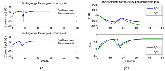
Figure 6.
The real-time tracking of trailing-edge flap angles and the real-time displacements controlled by pneumatic cylinders using optimal proportional–integral–derivative (OPID) theory: (a) The real-time tracking of trailing-edge flap angles; (b) The real-time displacements controlled by pneumatic cylinders.
From the fluctuations of real-time tracking curves of trailing-edge flap angles, the real-time tracking performance of OPID theory is poor, and both the rising time and the steady-state time are too large. The amplitudes fluctuations of the controlled displacements are also large compared with those in Figure 5. Especially for the fluctuations of the flap-wise displacements (z), the maximum amplitudes have exceeded 0.8 m, which may lead to the fracture failure of the blade under the actual working condition (compared with the blade length of 1.6 m). The superiority of the ASMC/MPLNN algorithm can be affirmed.
In addition, the trailing-edge flap control (TFC) method mentioned above can not only effectively control the vibration amplitudes of blade-tip displacements, but it can also have an effect on other parameters of the wind turbine, such as the energy efficiency, life cycle, aerodynamic noise, and so on. Of course, it also includes very few negative effects.
Let’s start with energy efficiency and the life cycle. The control target of TFC mainly focuses on the control of unstable aeroelastic behavior, rather than trying to obtain the maximum energy efficiency. As a result of the compromise between efficiency and stability, its essence is to reduce energy efficiency. According to the actual wind speed and the divergent degree of the unsteady movement of the blade tip, the energy efficiency can be reduced by 10% to 30%, and the greater the degree of instability of the blade, the more energy efficiency will be reduced with the increase of utility of vibration control. In contrast, the life cycle of the blade is extended greatly because the efficiency is reduced and the stability is ensured. In team members’ estimates, the blade life cycle can last at least 50% longer.
There are other beneficial effects, such as noise control. The aerodynamic noise is caused by the motion of the impeller and the air when the turbine is rotating normally, which produces pressure reactions and swirls to the air. An aerodynamic noise test was performed on a wind turbine with a rated power of 50 kW (which here refers to the case without a trailing-edged flap), compared to the test result after the trailing-edged flap was added. The sound sensor is placed in the center of the hub, and Figure 7 shows the noise contrast results measured by the sensor. It can be seen that with the increase of wind speed, the noise in both cases shows an increasing trend, but under the controlled cases using TFC, the noise level decreases obviously compared with the uncontrolled cases without a trailing-edge flap structure. As the wind speed increases, the distribution of the two kinds of noise appears to be close, which may be due to the increase of the mechanical noise brought by the control process of TFC, which affects the measurement results.
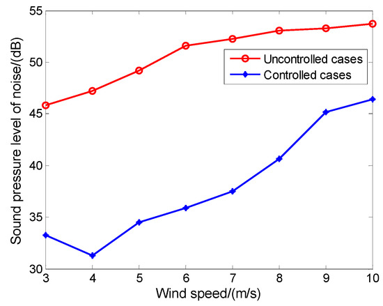
Figure 7.
The noise contrast results: sound pressure level of noise between uncontrolled cases and the controlled cases with trailing-edge flap structure.
5. Experimental Platform based on Pneumatic Transmission and Control System
Owing to the large wind power system being mostly controlled by PLC hardware, some intelligent control algorithms cannot be implemented in PLC hardware because of their complexity. For the purpose of engineering application, it is necessary to discuss the physical application of SMC/ARL and ASMC/MPLNN algorithms in Programmable Logic Controller (PLC) hardware and further confirm the physical effect of real-time control driven by pneumatic transmission. Figure 8 shows the experimental platform used for project implementation, with only the pneumatic unit at position l1 illustrated. The platform consists of Siemens PLC controller hardware system and the execution unit of pneumatic driving. The PLC system is composed of a CPU module, an analog module, a Human Machine Interface (HMI), and displacement sensors. The pneumatic execution unit in position of l1 is composed of a gas source processing unit, two proportional valves, a pneumatic pipeline system, pneumatic cylinders, and other accessory valve structures. The implementation scheme of the project is as follows:
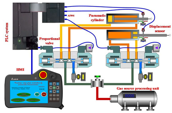
Figure 8.
The experimental platform used for project implementation.
(1) After starting the pneumatic pressure system, the CPU module (CPU 224XP) of PLC detects the two displacement signals of piston rods and the actual wind speed signal (in an AIW6 Channel) through the analog module (EM235), so as to determine the telescopic positions of the piston rods of the two pneumatic cylinders. The two actual displacement signals and wind speed signal are directly sent to computer via an Object Linking and Embedding for Process Control (OPC) technology using a PC/PPI (Personal Computer based on Point to Point Interface) cable [23]. This technology is exactly the virtual simulation technology; that is, it is an interactive simulation of PLC hardware and MATLAB software through an OPC Server.
(2) The aeroelastic equation of Equations (12) to (13) is modeled in MATLAB environment in a computer. The two adaptive SMC algorithms mentioned above run completely in PLC hardware. The results of variable execution and the calculated value of driving current are still transmitted to or from the PLC system through the OPC Server run on a computer.
(3) Signal interaction and variable transmission continue to occur periodically through the OPC Server. The spools of proportional valves move left and right continuously with the fluctuation of control currents , thus driving the piston rods of pneumatic cylinders to move continuously, synchronously, and reversely, so as to realize the control of angles of the trailing-edge flap.
(4) The driving currents of the two proportional valves are output by two different channels of the PLC system. One channel is provided by the analog output port of EM235 and the other is provided by the analog output port of the CPU224XP. The real-time values of the trailing-edge flap angles are reflected by the displacement values detected by sensors. There is an approximately proportional relationship between the angles and the displacements of piston rods, and the relationship coefficient is determined by the four-bar linkage mechanism. The displacement values of piston rods detected by sensors are displayed by HMI in time. The HMI device is connected to the 485 port of the CPU module.
Still, take the previous case for real-time tracking of trailing-edge flap angles under condition of in Figure 5a for example; Figure 9 shows the HMI interface and the physical displacements of piston rods detected by the sensor after the gain conversion in HMI, which represents the actual trailing-edge flap angles. The transverse coordinates in Figure 8 are time coordinates. Figure 9 shows only four frames of dynamic change of the trailing-edge flap angles with the change of time.
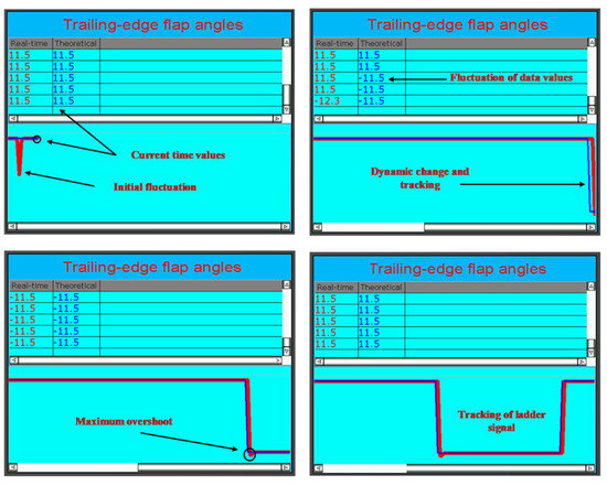
Figure 9.
The physical tracking effect of trailing-edge flap angles displayed in HMI.
Compared with the waveform of the real-time curve under in Figure 5a, the waveform of the physical trailing-edge flap angle (the control input ) detected by sensors in Figure 9 shows perfect consistency. The initial fluctuations of curves and the values of current time are displayed accordingly. The curves of dynamic change and tracking, and fluctuations of data values, are demonstrated in time. The maximum overshoot of real-time is displayed in the right place. The tracking effect of the ladder signal matches perfectly with that shown in Figure 5a. Compared with the real-time curve in Figure 5a, there are some subtle differences in the physical curve in the experiment. The differences are caused by the sampling time of the PLC hardware and HMI hardware. For instance, the value of the maximum overshoot in the experiment is smaller than that in Figure 5a due to the sampling time , omitting some actual data, but there is no deviation in the position of the overshoot.
The purpose of Figure 9 is to verify the feasibility of the theoretical control algorithms that can run perfectly in the actual PLC control hardware. In view of the specific requirements in this design, the aeroelastic model is completely running in the computer, and the operator only needs to detect the actual trailing-edge flap angle through the equivalent sensors in Figure 8. In addition, compared with the theoretical control input signal shown by Figure 4b under , the experimental result shown by Figure 9 is closer to that of Figure 4b, which further illustrates the effectiveness of the experimental scheme.
The consistency of the experimental results can confirm the following conclusions:
(1) The two adaptive SMC algorithms are effective.
(2) The two adaptive algorithms are feasible to be run in a PLC system, which lays a foundation of application for practical engineering problems.
(3) The driving planning of pneumatic transmission is feasible, which creates a new idea and control method for driving the trailing-edge flap.
(4) The reduced-order model is effective, which not only verifies the effectiveness of the Optimal Hankel Norm method, but also provides an effective way to deal with similar high-order physical systems.
6. Conclusions
The sliding mode control of an active trailing-edge flap for the large-amplitude vibrations of a CAS-based composite blade based on the adaptive reaching law and pneumatic transmission scheme is investigated. Some results are outlined as follows.
(1) The CAS-based composite blade, exhibiting displacements of flap-wise/twist coupling, is embedded in a rigid trailing-edge flap structure. The motion equations are solved using the Galerkin algorithm with the large amplitude vibration illustrated using time-response analysis.
(2) A refined thin-walled beam theory focused on CAS configuration and subjected to bending–twist coupling is investigated, with structural damping computed. If the structural damping is calculated, the high-frequency vibration of composite beams will be greatly suppressed (which is not specifically studied in this paper) and even show rapid convergence; however, the large-amplitude phenomenon in the vibration process will still occur. The control of this large-amplitude vibration is the purpose of this study.
(3) The active control of the trailing-edge flap is realized using the SMC/ARL algorithm based on an improvement adaptive discrete exponential reaching law. The execution results of the SMC/ARL algorithm can exactly match the control process of the pneumatic cylinders driven by pneumatic transmission.
(4) The pneumatic transmission system is a high-order system, which is transformed into a second-order system by the model reduction method. To make the change of the trailing-edge flap angles track the control input signals of the SMC/ARL algorithm, the ASMC/MPLNN algorithm is investegated to control the second-order system, so as to drive the action of the trailing-edge flap structure.
(5) The real-time realization of the two adaptive SMC methods is illustrated using the experimental platform via OPC technology. The remarkable effects of the physical tracking of the angles of the trailing-edge flap are illustrated by HMI in an experimental platform, which furthermore confirms the effectiveness of the control algorithms and the feasibility of the pneumatic transmission system.
Author Contributions
T.L. conceived the original idea; A.G. wrote and edited the manuscript; and C.S. and Y.W. supervised the study. All authors have read and agreed to the published version of the manuscript.
Funding
This research was funded by the National Natural Science Foundation of China, grant number 51675315.
Conflicts of Interest
The authors declare no conflict of interest.
References
- Song, O.; Librescu, L. Structural modeling and free vibration analysis of rotating composite thin-walled beams. J. Am. Helicopter Soc. 1997, 42, 358–369. [Google Scholar] [CrossRef]
- Chandiramani, N.K.; Shete, C.D.; Librescu, L. Vibration of higher-order-shearable pretwisted rotating composite blades. Int. J. Mech. Sci. 2003, 45, 2017–2041. [Google Scholar] [CrossRef]
- Silva, W.A.; Bartels, R.E. Development of reduced-order models for aeroelastic analysis and flutter prediction using the CFL3Dv6.0 code. J. Fluids Struct. 2004, 19, 729–745. [Google Scholar] [CrossRef]
- Xue, X.; Tang, J. Vibration control of nonlinear rotating beam using piezoelectric actuator and sliding mode approach. J. Vib. Control 2008, 14, 885–908. [Google Scholar] [CrossRef]
- Vadiraja, D.N.; Sahasrabudhe, A.D. Vibration analysis and optimal control of rotating pre-twisted thin-walled beams using MFC actuators and sensors. Thin-Walled Struct. 2009, 47, 555–567. [Google Scholar] [CrossRef]
- Arvin, H.; Nejad, F.B. Nonlinear free vibration analysis of rotating composite Timoshenko beams. Compos. Struct. 2013, 96, 29–43. [Google Scholar] [CrossRef]
- Rafiee, R.; Tahani, M.; Moradi, M. Simulation of aeroelastic behavior in a composite wind turbine blade. J. Wind Eng. Ind. Aerodyn. 2016, 151, 60–69. [Google Scholar] [CrossRef]
- Chang, L.; Xu, W.; Wu, H. Research and optimal control of blade aeroelastic stability of large horizontal axis wind turbine. Mach. Des. Res. 2018, 34, 199–204. [Google Scholar]
- Akbar, M.A.; Mustafa, V. A new approach for optimization of Vertical Axis Wind Turbines. J. Wind Eng. Ind. Aerodyn. 2016, 153, 34–45. [Google Scholar] [CrossRef]
- Haselbach, P.U. An advanced structural trailing edge modelling method for wind turbine blades. Compos. Struct. 2017, 180, 521–530. [Google Scholar] [CrossRef]
- Llorente, E.; Ragni, D. Trailing-edge serrations effect on the performance of a wind turbine. Renew. Energy 2020, 147, 437–446. [Google Scholar] [CrossRef]
- Chen, H.; Qin, N. Trailing-edge flow control for wind turbine performance and load control. Renew. Energy 2017, 105, 419–435. [Google Scholar] [CrossRef]
- Huang, X.; Moghadam, S.M.A.; Meysonnat, P.S.; Meinke, M.; Schröder, W. Numerical analysis of the effect of flaps on the tip vortex of a wind turbine blade. Int. J. Heat Fluid Flow 2019, 77, 336–351. [Google Scholar] [CrossRef]
- Thakur, S.; Abhinav, K.A.; Saha, N. Stochastic response reduction on offshore wind turbines due to flaps including soil effects. Soil Dyn. Earthq. Eng. 2018, 114, 174–185. [Google Scholar] [CrossRef]
- Liu, T. Quadratic feedback–based equivalent sliding mode control of wind turbine blade section based on rigid trailing-edge flap. Meas. Control 2019, 52, 81–90. [Google Scholar] [CrossRef]
- Bianchini, A.; Balduzzi, F.; Rosa, D.D.; Ferrara, G. On the use of Gurney Flaps for the aerodynamic performance augmentation of Darrieus wind turbines. Energy Convers. Manag. 2019, 184, 402–415. [Google Scholar] [CrossRef]
- Zhang, Y.; Ramdoss, V.; Saleem, Z.; Wang, X.; Schepers, G.; Ferreira, C. Effects of root Gurney flaps on the aerodynamic performance of a horizontal axis wind turbine. Energy 2019, 187, 115955. [Google Scholar] [CrossRef]
- Kumar, P.M.; Samad, A. Introducing Gurney flap to Wells turbine blade and performance analysis with OpenFOAM. Ocean Eng. 2019, 187, 106212. [Google Scholar] [CrossRef]
- Chen, X.; Xu, J.Z. Structural failure analysis of wind turbines impacted by super typhoon Usagi. Eng. Fail. Anal. 2016, 60, 391–404. [Google Scholar] [CrossRef]
- Zhuang, C.; Yang, G.; Zhu, Y.; Hu, D. Effect of morphed trailing-edge flap on aerodynamic load control for a wind turbine blade section. Renew. Energy 2020, 148, 964–974. [Google Scholar] [CrossRef]
- Calkins, F.T.; Mabe, J.H. Flight test of a shape memory alloy actuated adaptive trailing edge flap. In Proceedings of the ASME 2016 Conference on Smart Materials, Adaptive Structures and Intelligent Systems, Stowe, VT, USA, 28–30 September 2016. [Google Scholar]
- Zhou, X.; Huang, K.; Li, Z. Geometrically nonlinear beam analysis of composite wind turbine blades based on quadrature element method. Int. J. Non-linear Mech. 2018, 104, 87–99. [Google Scholar] [CrossRef]
- Liu, T. Dynamic Stall Aeroelastic Stability Analysis and Flutter Suppression for Wind Turbine Blade; Golden Light Academic Publishing: Beau-Bassin, Mauritius, 2017; pp. 19–43, 95–136. [Google Scholar]
- Gu, Y. Study on Optimization Design Method of Wind Turbine Blade; Zhejiang University: Hangzhou, China, 2014. [Google Scholar]
- Liu, T. Vibration and aeroelastic control of wind turbine blade based on B-L aerodynamic model and LQR controller. J. Vibroeng. 2017, 19, 1074–1089. [Google Scholar] [CrossRef]
- Dancila, D.S.; Armanios, E.A. The influence of coupling on the free vibration of anisotropic thin-walled closed-section beams. Int. J. Solids Struct. 1998, 35, 3105–3119. [Google Scholar] [CrossRef]
- Saravanos, D.A.; Varelis, D.; Plagianakos, T.S.; Chrysochoidis, N. A shear beam finite element for the damping analysis of tubular laminated composite beams. J. Sound Vib. 2006, 291, 802–823. [Google Scholar] [CrossRef]
- Barambones, O.; Alkorta, P.; Durana, J.M.G. A real-time estimation and control scheme for induction motors based on sliding mode theory. J. Frankl. Inst. 2014, 351, 4251–4270. [Google Scholar] [CrossRef]
- Claudiu, P.; Radu-Emil, P. An approach to the design of nonlinear state-space control systems. Stud. Inform. Control. 2018, 27, 5–14. [Google Scholar]
- Liu, J. Sliding Mode Control Design and MATLAB Simulation the Basic Theory and Design Method, 2nd ed.; Tsinghua University Publishing Company: Beijing, China, 2017; pp. 460–480. [Google Scholar]
- Kong, X. Research and Application of Pneumatic Intelligent Control System; Chemical Industry Press: Beijing, China, 2019; pp. 36–56. [Google Scholar]
- Xue, D. Computer Aided Control Systems Design Using MATLAB Language, 3rd ed.; Tsinghua University Publishing Company: Beijing, China, 2012; pp. 50–53. [Google Scholar]
- Alvarez-Gil, R.P.; Johanyák, Z.C.; Kovács, T. Surrogate model-based optimization of traffic lights cycles and green period ratios using microscopic simulation and fuzzy rule interpolation. Int. J. Artif. Intell. 2018, 16, 20–40. [Google Scholar]
- Pedro, J.O.; Nyandoro, O.T.C.; John, S. Neural network-based feedback linearisation slip control of an anti-lock braking system. In Proceedings of the 7th Asian Control Conference, Hong Kong, China, 27–29 August 2009; pp. 1251–1257. [Google Scholar]


© 2020 by the authors. Licensee MDPI, Basel, Switzerland. This article is an open access article distributed under the terms and conditions of the Creative Commons Attribution (CC BY) license (http://creativecommons.org/licenses/by/4.0/).