Abstract
Targeting existing residential buildings for retrofit improvement presents significant prospects for global reduction of energy-usage and carbon footprints. Energy consumption of the existing single-family building in the hot-humid climate zone needs to be targeted for improvement due to their potential energy-savings and sizeable market share. This paper proposes and evaluates energy savings and cost-effectiveness of a whole building retrofit package for single-family residential buildings built between 1950 and 1970. The study outlined a survey conducted using the clustering data mining technique on Florida Single-Family Residential (SFR) homes to determine the essence of the building envelope, patterns of construction, and Heating, Ventilation, and Air-Conditioning (HVAC) systems. The evaluation of the energy efficiency measures (EEMs) effectiveness is performed utilizing Autodesk Revit and a Six-Step modeled framework. This framework consists of baseline model development, validation of the model with an actual case study building, identification of potential EMMs, evaluation of EEMs individually and incorporating the selected EMMs into retrofit package and maximizing the energy-saving and cost-effectiveness of the proposed retrofit package. The study develops proposed retrofit improvement package detailing replacement & improvement EEMs, implementation cost, annual energy savings (kWh), cost-saving ($), and payback period (years) for each individual EEM as well as the combined/total energy improvement package. The paper further explored the usage of solar photovoltaics (PV) energy generation options to offset the remaining energy-use after the implementation of the proposed retrofit package.
1. Introduction
The growing concerns about climate change and continuous rise in energy cost have prompted public interest in energy efficiency and conservation measures. According to the Energy Information Authority (EIA) [1], the total energy consumption in the United States for both residential and commercial sectors contributed about 40% (or about 40 quadrillion British thermal units) in 2018. Residential buildings utilize 22% of total consumption in the United States from which Single-Family residential buildings are responsible for 80% total energy consumed, multi-family buildings consumed 15%, and 5% consumption is attributed to mobile homes. The diversity of energy consumption across the United States is as a result of the different home types, sizes, structures, and climate zones [2]. A survey conducted by the United States Census Bureau 2013 [3] found that more than 60% of the United States’ housing stock is 30 years old and energy inefficient and consumes more energy compared to new buildings [3]. There is a need to address the existing residential building stocks to reduce the high energy consumption, focusing on older single-family residential homes [4]. Emrath et al. [5] concluded in their study that the newer the house, the less energy it uses per unit area basis.
Wang et al. [6] defined energy retrofit as the physical and operational change of a building itself, its energy end users, or occupants’ behavior. They found that a combination of passive and active measures can be adopted to achieve the required levels of energy efficiency. Active measures offer the necessary flexibility to cut-down the excess costs of the utility bills through continuous monitoring while passive strategy scrape pares unnecessary surplus energy consumption. Betharte et al. [7] studied the effect of various potential passive and active EEMs for energy efficiency improvement of an office building in Melbourne, FL. They selected the most promising EEMs based on their potential for energy savings as well as estimated implementation cost and achieved about a 50% reduction in total annual building energy consumption. D’Agostino et al. [8] used EnergyPlus to determine the impacts of passive and active approaches on energy savings in buildings and concluded that passive building design strategies should be prioritized. The authors found the effectiveness of active strategies in terms of total energy reduction varies between the original design and the re-design. Fairey et al. [9] examined the opportunities for cost-effective energy efficiency and renewable energy retrofits in residential archetypes constructed before 1980 (pre-code) in 14 U.S cities. The critical finding from [9] investigation indicated that the energy efficiency of even older, poorly insulated homes across U.S. climates could be improved dramatically with favorable economics, they can reach performance levels of near net-zero energy when assessed on an annual basis. Also, the indication in their findings stated retrofit financing alternatives and whether equipment requires replacement had a considerable impact on the achievable source energy reduction.
Despite the number of different entities providing resources on the retrofit process, the research into this vital subject matter influencing decision remains limited. The selection process of a retrofitting strategy is a trade-off between the capital investment and the benefits derived from energy retrofitting. These energy retrofitting benefits can be economical, environmental, or social (enhancing occupants’ comfort and health) [10].
Building Energy Retrofit in Hot-Humid Climate
Building researchers and industry professionals have made significant efforts towards the development and application of various retrofit technologies and decision support tools to enhance building energy performance. This section relates to the study conducted in terms of energy efficiency retrofits, energy modeling/analysis, and economic analysis in hot-humid climates.
McIlvaine et al. [11] conducted a study in central Florida to examine the efficiency of retrofit opportunities, typical renovation practices, and pathways for achieving U.S. Department of Energy (DOE) goals of energy-efficient existing homes for the region. The authors conducted renovation activities on 70 foreclosed homes built from the 1960s through the 2000s.The average improvement for the 70-house dataset was a 34% decrease in the Home Energy Rating System (HERS) index. Annual average projected energy cost savings were 25%. Silvero et al. [12] evaluated the thermal performance of a dwelling located in a humid climate. The authors assessed several retrofitting solutions for the building envelope to determine the most efficient solution for the building and the climate zone. The results indicated that the implemented strategy contributed to the reduction of the overheating problem of the building and maintained comfortable indoor conditions adding to the improvement of occupant well-being. Burgett et al. [13] demonstrated the application of energy simulation as an effective tool for specifying cost-effective residential packages that will reduce energy consumption by 30%. The authors used single-family buildings in the hot-humid climate in the southern USA to demonstrate the application. The study found that replacing lights with CFLs, installing low-flow water fixtures, providing programmable thermostats, applying window films, and reducing standby power loss were constantly cost-effective. The study recommended that if all EEMs proposed were implemented together, the energy use would reduce from 20% to 25% with a simple payback period of fewer than two years. The study also highlighted the value that computer simulation models could have on the development of energy efficiency packages and cost-effectiveness in relation to homeowner’s, location and housing type. Retrofitting existing buildings offers significant opportunities for reducing global energy consumption and greenhouse gas emissions [14]. Ma et al. [14] evaluated a systematic approach to proper selection and identification of the best retrofit options for existing buildings. The authors suggested a whole building retrofit with comprehensive energy simulation, economic analysis, and risk assessment as an effective approach to identify the best retrofit solutions. The authors further recommended more research and investigation to facilitate energy and cost-effective building retrofits. Al-Saadia et al. [15] investigated different energy-efficient retrofitting strategies, including insulation for both walls and roof, upgrading to LED lights, and improving the air tightness. The study concluded that, when combining the best strategy from each category, the annual energy consumption can be reduced as much as 42.5%. Alam et al. [16] carried out a comprehensive review of barriers to retrofitting guidelines and progress. The authors categorized barriers to energy retrofitting as regulatory, economic, knowledge, or social. The study found, existing research, had shown the importance of conducting a risk assessment in building a retrofitting process. None of the currently available retrofit guidelines includes a risk assessment. Also, some guidelines have no recommendation for post-occupancy evaluation of installed retrofit measures. Goldman et al. [17] introduced energy savings and the cost of conservation measures in U.S. multifamily buildings based on the analysis of measured data of over 25,000 dwelling units. The majority of the processes can be applied to single-family homes. Median energy savings were 1450 kWh/unit in electric-heated buildings and 14 MBtu/unit in fuel-heated buildings. The results show that the retrofit costs of ($370/unit) for fuel-heated buildings were much lower than that of electric-heated buildings ($1600/unit). The payback periods for fuel-heated buildings and electric-heated buildings were six years and 20–25 years, respectively. Deep Energy Retrofit (DER) performance in the U.S. has been assessed in 116 homes in the United States [18], using actual and simulated data gathered from the available domestic literature. The results indicated that annual energy costs were reduced by $1283 ± $804 from a pre-retrofit average of $2738 ± $1065 to $1588 ± $561 post-retrofit. These results provide estimates of the potentials of deep energy retrofits to address energy use in existing buildings. Building Energy Optimization Tools (BEopt) has been used extensively in the U.S. Department of Energy’s Building America program to direct research, assess emerging technologies, evaluate innovative prototype buildings, and estimate energy savings potential [19]. According to Christensen et al. [20], BEopt software is designed to find optimal building designs along the path to Zero Net Energy [20], the software provides either a user-defined base-case building or a climate-specific Building America Benchmark building automatically generated by BEopt and the user can also review and modify detailed information on all available options in a linked options library spreadsheet. Simulations of building energy use can give insights into how energy efficiency retrofits and operational changes can influence a building’s total and temporal energy use [20]. Rhodes et al. [21] determined model accuracy by considering 54 homes in Austin, TX, that are part of a smart grid demonstration project. Lee et al. [22] investigated retrofit tools both in the public domain as well as in the private sector to better understand the diverse approaches currently in use to evaluate retrofit methods, measures, interoperability, target audiences, as well as interface types and accessibility. Shabunko et al. [23] used the EnergyPlus simulation tool to benchmark the energy performance of 400 residential buildings from which three types of buildings were classified. The EnergyPlus models produced the energy use intensity (EUI) per year for these buildings, with values ranging from approximately from 64.2 to 47.8 kWh/m².
An economic analysis that facilitates the comparison among alternative retrofit measures can indicate whether the retrofit alternatives are energy-efficient and cost-effective. Jafari et al. [24] proposed a decision-making framework that calculates the economic benefits of energy retrofitting in terms of reduction of life-cycle cost for a specific building during its service life and determines the optimum retrofitting budget that minimizes the total life-cycle cost of the building during its service life. The framework also allows for the selection of optimum energy retrofitting strategies (among available energy retrofitting measures) to maximize the homeowner’s economic benefits during the service life of the building. According to the Whole Building Design Guide (WBDG) Cost-Effective Committee [25], an economic analysis was performed for six formulated refurbishment scenarios to determine which of the scenarios will demonstrate optimal performance both in energy and cost-efficiency. A variety of economic analysis methods were used to evaluate the economic viability of building retrofit measures. Some of them, such as net present value (NPV), internal rate of return (IRR), overall rate of return (ORR), benefit-cost ratio (BCR), discounted payback period (DPP), and simple payback period (SPP), can be used to assess the economic feasibility of a single retrofit measure. Alternatively, the life cycle cost method, the levelized cost of energy, and other advanced analysis methods can be used to evaluate the cost-effectiveness of multiple retrofit alternatives [25,26]. All sectors of the energy community need guidelines for making economically efficient energy-related decisions [27]. Beyond social responsibility, more and more data are making it clear that it makes economic sense for landlords to retrofit their buildings and make them sustainable and energy-efficient [28]. A dynamic investment analysis utilizing the discounted cash flow (DCF) method was conducted for a series of energy-efficient retrofit packages that were applied to a specific model building [29]. The investigation provided a rational basis for decisions by house owners. Nguyen et al. [30] proposed an approach to enhance data interoperability to allow for seamless integration of design and energy analysis processes. The authors used Autodesk Revit software to design a BIM-Based architectural model as a case study. The study found that a suitable combination of design, energy modeling, and data exchange interface tools will help improve the project cost and schedule overruns.
The literature, as described above, portrays the very diverse nature of energy retrofit and also the influences of numerous uncertainty factors. A favorable prediction of the uncertainty factors regarding the choice and combination of the proposed EEMs is vital to help select the best retrofit option to maximize the building energy efficiency during its whole service life.
2. Methodology
The methodology for this research adopted an approach that includes an extensive study targeted at improving the energy performance of existing single-family residential buildings in the state of Florida, which also applies to other hot-humid climate zones. The purpose is to establish energy efficiency measures (EEMs) capable of reducing building energy consumption coupled with the lowest retrofit cost. This section develops six-step modeled framework that includes: the baseline model definition; verification of the model with an actual building; identification of the EEMs; estimating the cost of the EEMs; evaluating the effectiveness of the EEMs; and eventually developing the retrofit package aligned with the objective of this study.
2.1. Define Baseline Model
An actual building is considered to represent the target class of single-family residential buildings. The building is modeled via Autodesk Revit (Autodesk, Inc., San Rafael, CA, USA) and used as the case study building for further analysis. The case study building was built in 1959 and has an approximate footprint of 168 m². Section 4 provides a full development of the baseline model.
2.2. Verify Baseline Model with the Actual Data
The verification process is performed by comparing the predicted energy consumption data to the actual electric bill data. A meter-level utility data, i.e., an average monthly electric bill for the year 2018 with an annual energy consumption of 19,081 kWh/year, was the basis of comparison for the simulation analysis.
2.3. Identify EEMs
Identification of EEMs depends mostly on the results of an energy audit conducted in Section 4.1. and energy end-use estimate process as described in Section 4.4. These two activities presented the real state of the case study building that led to the identification and selection of the EEMs.
2.4. Estimate the Cost of EEMs
The initial retrofit cost is an essential determinant for the selection of a proposed EEMs. The cost estimate for the EEMs is performed using industry published data such as RSMeans [31], manufacturers cost/user guide and vendor prices provided by national retail vendors the reliance of local general and subcontractors, as well as historical data from previous projects.
2.5. Evaluate the Effectiveness of EEMs
This step deals with the simulation of the energy savings of the selected EEMs. Multiple simulations of EEMs are performed to predict the optimal retrofit package with the highest cumulative energy savings, which corresponded with the lowest up-front cost.
2.6. Develop Retrofit Package
The procedure for developing the retrofit package is fully described in Section 6. The approach defines a customized automation process of selecting and simulating the individual EEMs making up the combined retrofit package. Figure 1 shows the summarized six-step modeled framework for the methodology as described above.
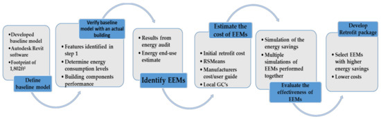
Figure 1.
Six-Step modeled framework approach.
3. Single-Family Building Survey for Florida
A survey of Florida Single-Family Residential (SFR) buildings constructed between the years 1950 and 1970 was conducted to collect data associated with the properties. The search aimed at establishing each building’s architectural style, roof profile, building envelope type, and HVAC system type. The study used the Clustering data mining technique for the search of property appraisal databases. Clustering, also called data segmentation, as large data groups are divided by their similarities. A total number of 2,621,262 residential buildings were surveyed through the property appraisal database across the sixty-seven counties in Florida [32,33,34,35,36,37,38,39,40,41,42,43,44,45,46,47,48,49,50,51,52,53,54,55,56,57,58,59,60,61,62,63,64,65,66,67,68,69,70,71,72,73,74,75,76,77,78,79,80,81,82,83,84,85,86,87,88,89,90,91,92,93,94,95,96,97,98]. Table 1 shows the breakdown of data for each county. Out of the total number surveyed, the authors selected 6,700 buildings for further analysis. Figure 2, Figure 3, Figure 4 and Figure 5 provides results of typical exterior walls, roofing, windows, and building footprints, respectively. Figure 2 shows 85% of the buildings use concrete masonry units (CMU) as exterior walls, while Figure 3 shows 90% of the roofing types are asphalt shingles. Figure 4 indicates two major types of windows of which, single-pane windows constitute 80%. Figure 5 shows the average footprint of all buildings across the counties. The buildings’ square footage is grouped into seven categories according to the sizes of the buildings’ footprints as the indicated figure below. The majority of the building footprints, according to the survey results, are centered between 186 m² and 279 m², respectively. The majority of the buildings, 92%, uses a central air-conditioning HVAC system while 8% attributed to Heating Force-Air. 95% of the homes have an electric power source. There was no information discovered on lighting systems and fixtures. Other patterns related to the building shape include rectangular, "L or U" shape, and or low pitch roof with extended eaves. They have an attached garage and a large picture window facing the street. The houses are generally three (3) bedrooms on average across all counties. The buildings’ exterior features are predominantly made of masonry concrete blocks, as indicated in Figure 2 for exterior walls types, drywall for interior partition, slab-on-grade, and carpet, or vinyl for floor. Based on the age of these buildings, it is safe to assume that the majority of them are energy inefficient. About 80% of the windows are a single uninsulated pane, evident from their visibly deteriorated nature. Some of the gaping holes noticed along the joints of the building envelopes make it reasonable to say that they are not sealed correctly from the air leakages.

Table 1.
Single family residential (SFR) building survey from each county.
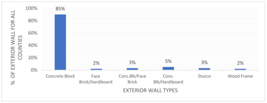
Figure 2.
Type of exterior walls.
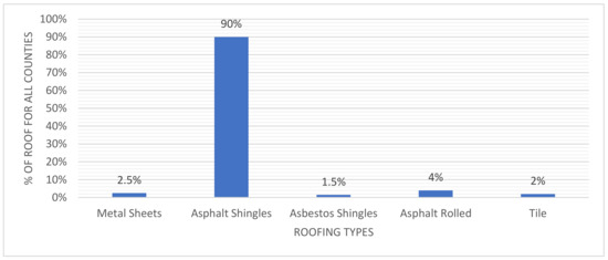
Figure 3.
Type of roof materials.
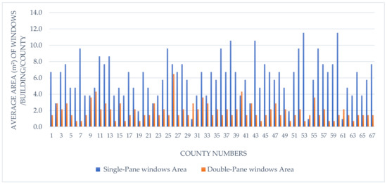
Figure 4.
Per unit area of windows and types for selected buildings in each county.
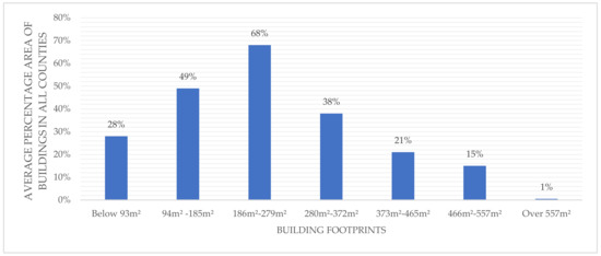
Figure 5.
Average areas of building footprints grouped from the smallest to the largest sizes.
4. Baseline Model
A residential building located in Melbourne, FL (28.070071, 80.525198), was chosen as a baseline for the study. Concrete block walls, asphalt shingle roofing, single pane glazed windows, and wood/aluminum frame glass doors make up the predominant features of the building envelope. These characteristics represent approximately 85% of the features discovered through the single-family residential survey conducted by the authors. The majority of counties have a similar type of structure. Five people occupied the building, two adults, and three children. The residence was built in 1959 with a 168 m² footprint, including both conditioned and unconditioned (garage) areas, 1133 m² lot size, three bedrooms, and two baths. The building has one HVAC system type: a “Package Terminal AC with electric resistance heat,” including DX coils as a cooling source and electric resistance for a heating source. An EER of the Terminal HVAC unit was 11.3 found from the manufacturer’s label. Zone group definitions were used to allocate the HVAC units. The HVAC system operates all day.
Table 2 shows the window-to-wall ratio (WWR) of the building and the window types installed. WWR is an essential variable affecting energy performance. The building has a light color strip asphalt shingle on a wooden rafter. The energy audit Section 4.1, outlines the detailed characteristics of the building.
Table 2.
Window-to-wall ratio.
A baseline must be defined appropriately in order to accurately determine the effectiveness of the EEMs in next steps. The authors developed a model based on the actual building using Autodesk Revit as shown in Figure 6 and Figure 7. With the aid of the Autodesk Revit, the model was created to support the energy modeling and simulation analysis process for the determination of the cost-effectiveness and energy efficiency of the chosen EEMs/retrofit package.

Figure 6.
The baseline building model in Revit.
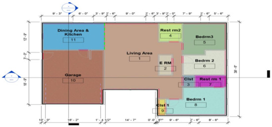
Figure 7.
Floor layout of the baseline building.
4.1. Energy Audit
A level 1 energy audit to ASHRAE Standards was conducted on the case study building to understand baseline energy consumption, end users and potential energy-related opportunities. The main components observed throughout the audit process include:
- Primary Energy Use Analysis (PEA);
- Walk-through survey;
- Identifying low-cost/no-cost energy saving opportunities;
- Identifying capital improvements.
The survey was administered three times within six months to obtain the actual data for the building. Total Annual Energy Use (kWh/m²) per the Florida Power and Light (FPL) bills was 19,018 kWh/m² for the year 2018. During the walk-through excise, we posed a series of questions to the owner and the other occupants. The electricity bills for two years (2017 and 2018) were obtained from the owner to conduct the actual energy usage analysis. Table 3 depicts the summary of monthly and annual energy consumption breakdown and cost. More detailed energy audit on the equipment, lighting fixtures, and HVAC units was necessary to establish the point of reference for the energy analysis. Manufacturers’ data sheets played a significant role in developing a credible schedule for the baseline building. There were no energy-efficient light fixtures. Table 4, Table 5, Table 6, Table 7 and Table 8 presents the summarized findings of the energy audit. Table 4, Table 5, Table 6, Table 7 and Table 8 contains the windows schedule, list of exterior doors, plug loads, equipment, lighting schedule, and Heating/Cooling set-points, respectively.
Table 3.
Summary of Utility Bills for 2017 and 2018.
Table 4.
Window characteristics.
Table 5.
Exterior doors characteristics.
Table 6.
Plug loads and equipment.
Table 7.
Lighting systems.
Table 8.
Heating/cooling set-points in Fahrenheit.
4.2. Energy Modeling and Simulation Process
Energy modeling plays a vital role in determining potential energy savings from retrofit projects. To reliably predict energy savings from a class of identified EEMs, the energy simulation model must represent the building’s operational characteristics. Hence, the energy audit and the measured electricity consumption also become integral to the modeling process. If the baseline model can generate outcomes that closely match monitored energy consumption of the building, then it is likely to predict reliable estimates of the energy savings from the planned retrofits. This section takes a Whole-Building detailed modeling approach to estimate the energy use and also defines the energy performance of each EEM/proposed retrofit package.
Different levels of energy settings are necessary to establish the bases for the simulation analysis, including the building type, location, and average energy cost. The following settings are specifically made to model; the building type is single-family; the assign location is Melbourne, FL (latitude 28.07, and longitude 80.60) as well as the energy cost of $0.1142/kWh/m². The authors created eleven spaces and two thermal zones for the model. The occupancy schedule was set to home occupancy (24 hours occupancy), lighting, and power schedule was set to residential light (All Day). Cooling and heating set-points were set at 78.00 °F and 60.00 °F year-round. The building infiltration class was set to “medium.” All lights fixtures/bulbs were changed from incandescent/ compact bulbs to LED lights (15 Watts) as part of the retrofit process. These and other assumptions made at the later stages of the simulation analysis served as a basis for all the comparative analysis for the retrofit scenarios considered. The Revit architectural baseline model was link to MEP Revit template for all the energy simulation analysis. We used both Revit architectural and the MEP model as a simulation tool to create the baseline model. In the MEP model, spaces were created and assigned to the thermal zone(s). Each area (space) created tagged to a specific room with detailed designated functions. It is vital to create spaces with assign zones to help manage the simulation and data export. The detailed results of the data sent through gbXML are analyzed by Green Building Studio (GBS) over the cloud. Any input made into the baseline model will yield the resultant output.
4.3. Actual and Baseline Energy Use
To verify the model, as shown in Figure 8, the monthly electric bill data for 2018 are obtained from the utility company and compared against the calculated values from the model. The model result is in very good agreement with the actual utility bill consumption data. This section, including Section 4.4 and Section 4.5, plays a vital role in the selection and application of the EEMs.
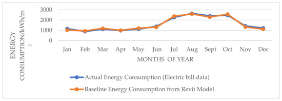
Figure 8.
Comparison between actual and baseline energy usage.
4.4. Energy End Use Estimate
The energy end-use estimate is developed, as shown in Figure 9 is as a result of the energy audit conducted in Section 4.1. using Autodesk Revit.
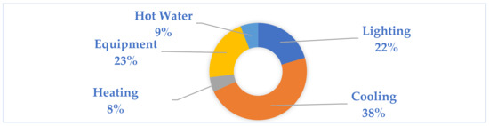
Figure 9.
End-use energy estimate.
The cooling system is the largest energy end-user, followed by lighting systems and equipment loads. Hot water and heating loads shared the lowest consumption levels, respectively. The End-Use analysis presented the opportunity for the authors to properly defined EEMs for areas that demand more attention in terms of energy consumption. (Cooling, lighting, and equipment). The results of this energy end-use estimates serve as bedrock for decision consideration regarding the selection of the EEMs. Cooling and heat gain sources are further analyzed, i.e., generating the heating and cooling loads from Revit to determine the true origin of the loads. Section 4.5. discusses in detail, the cooling and heat gain sources.
4.5. Cooling Loads and Heat Gain Sources
Figure 10 demonstrated the distribution of sources of cooling load. As seen, the largest source of cooling load are the windows followed by roof/attic. It is vital to understand the load sources regarding these end-uses in a typical Florida SFR building.
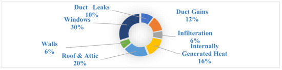
Figure 10.
Cooling Load Sources.
5. Selection of Energy Efficiency Measures (EEMs)
This section defines different simulation analysis of the EEMs. The categorization of the EEMs is according to passive and active measures. The recommendations of the EEMs that form part of the final retrofit package is based on analyzing the existing energy end-use, as estimated from the energy model of the case study building. As shown in Figure 9, the largest end-use are cooling and lighting, which presented the most significant opportunity for savings. Hence, the recommended package focused on prioritizing the EEMs that could reduce the energy used for cooling and lighting systems.
The first target was to increase the insulation quality, decrease the infiltration, and bring the equipment/ducts into the conditioned space by insulating the radian barriers on the attic of the roof. To further improve the envelope, the authors conducted a simulation analysis to select a high-performance wall and roof insulation as well as windows with proper U-Values and very low solar heat gain coefficients (SHGCs).
Figure 11 and Figure 12 show the addition of wall and roof insulations modeled in Revit with varying thickness to simulate different R-values for the exterior walls ranging from 7.5 to 19 with roofing insulation ranged from R-11 to 40 respectively.
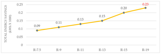
Figure 11.
The impact of using additional wall insulation on total annual electricity consumption of a building.
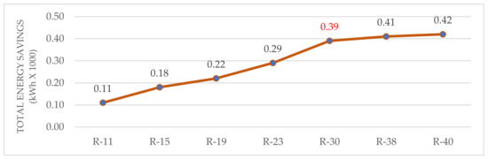
Figure 12.
The impact of additional roofing insulation on the total annual electricity consumption of the building.
The inclusion of the exterior wall insulation is a way to slow down the heat transfer process through the wall. In hot-humid climate like Florida, the temperature difference between inside and outside of the building is relatively small, which in turn alleviates the impact of using materials with high thermal resistance for walls and roofs on the energy consumption of the building. Energy simulation analysis is performed to assess the effect of roof insulation on building energy performance (Figure 12). The addition of roof insulation R-values ranged from 11 to 40 as marginal changes can be seen between R-30 (390 kWh/year), R-38 (410 kWh/year), and 40 (420 kWh/year).
A significant amount of heat loss or gain in buildings occurs through the windows. Heat gain through windows takes place in two different heat transfer modes: radiation and conduction. The energy consumption of buildings varies significantly as a result of using different types of windows. The baseline building uses both single and double pane uninsulated clear conventional windows. The authors assumed that energy-efficient windows replace all windows. The energy-efficient window technologies considered for the analysis include; single & double pane clear, single & double low-E, and single & double reflective tint, respectively. Figure 13 draws the comparison between the potential energy savings as a result of using different energy-efficient window glasses. Although the double-pane reflective tinted offers significant energy savings of 2403 kWh/year, representing 21% of the energy savings, the single-pane reflective tint window offered the most promising savings in terms of cost-effectiveness, thus saving 2353 kWh/year (20%). The reflective tint reflects the non-visible part of the solar radiation, which in turn reduces the solar heat gain that leads to a reduced cooling load in the summer months and therefore, would be an excellent choice for hot-humid climates.
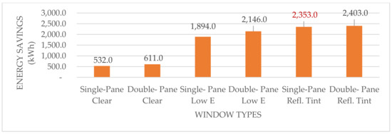
Figure 13.
Annual energy savings per using different type of energy efficient windows.
An active strategy of improving HVAC efficiency for building energy performance ranks among the highest in potential energy savings. The cooling efficiency is measured by its SEER (Seasonal Energy Efficiency Ratio) value. A higher SEER value improvement would lower the energy consumption of the cooling system. The efficiency of the heating system is identified by COP value or HSPF (Heating System Performance Factor). Just as SEER, the effectiveness of the heating system increases with the increase of the COP. Figure 14 demonstrates the effect of an improved efficiency of the HVAC unit on the total energy savings. As the diagram shows, when the SEER value increases from SEER 9 to 21, energy savings in the amount of 3465 kWh/year can be realized, representing approximately 25%. SEER 17 considered appropriate for the selected EEM because it offered a significant energy savings of 2379 kWh/year (23%) compared to SEER 21 in terms of cost-effectiveness.
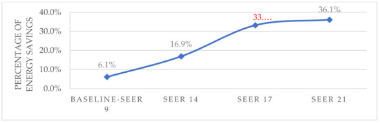
Figure 14.
The effect of variation of SEER value on the total annual energy consumption of the building.
By adding insulation to the exterior walls and properly sealing around windows, infiltration was anticipated to decrease to 4 air changes per hour (ACH) at 50 Pascal instead of 6 ACH. The simulation confirmed infiltration at approximately 3.8 ACH 50, yielding 578 kWh/year energy savings (3%). The introduction of R-6 ducts with leakage of 7.5% central return to bring fresh air into the building incurred a slight reduction of the energy savings of 3.5% in the simulated retrofit package consumption from 63.6% to 60.1%. However, this system also provides dehumidification, so the improvement to indoor air quality was worth the small reduction in energy savings. The dehumidifier may enable occupants to use a higher cooling set point that will offset the energy consumption with cooling savings. Table 9 shows additional consideration for the simulation analysis, including annual energy savings. Reducing heating set points and increasing cooling set points produced 298 kWh (3%), while the introduction of the Programmable Thermostat yielded 910 kWh/year representing 7.8%.
Table 9.
Proposed Retrofit Improvement Package.
The current lighting of the existing building is T8 fluorescent tubes rated at 32 W. The LED light replacements consume approximately 12 W of power. The entire lighting in the case study building is replaced with LED lighting for the simulation analysis. No outdoor/task lighting was taken into consideration. The simulation results for lighting replacement yielded a savings of 2348 kWh/year, approximately 19.2% of the total energy consumption of the building. It should be noted that replacing the lights with LEDs did not only reduced the energy consumption of the lighting system, but also brought additional savings on the heating and cooling loads by reducing the total heat gain
The introduction of occupancy sensors/dimmers reduced the actual occupancy from 100% to 85%, resulted in an energy-savings of 967.6 kWh/year (8.3%).
As shown at the bottom half of Table 9, additional energy-savings measures using solar PV panels are available to owners who want to transform their building into near-zero or zero energy building. Appendix A, Table A1 and Figure A1demonstrates the detailed process of solar PV analysis. The analysis shows the solar system size (KW), average annual production (kWh), an estimated number of panels with percentage savings. The available options include choosing between 14 solar panels with 4954 kWh/year for a system size of 3.5 kW up to 69 solar panels providing 21,234 kWh/year with 15 kW system size depending on the owner’s preference. Opting for the PV option should be considered after the implementation of the main recommended retrofit improvement package. Adding solar PV panels may incur an additional cost and would be beneficial to owners whose sole aim is achieving high-performance building. Nonetheless, the benefits of solar PV addition may help to prevent long power outages due to environmental hazards.
6. Retrofit Package
The procedure for the retrofit package development is illustrated in Figure 15. This process is similar to how an energy auditor or home performance contractor may develop a recommended retrofit package. The diagram demonstrates a customized process for selection and simulation of a combined retrofit package/individual EEMs capable of meeting energy reduction and cost-effectiveness in SFR buildings. For each EEM, the cost-effectiveness is evaluated by calculating the payback period. The simple payback period (SPP) of each EEM was calculated using the following equation: SPP = (Implemented cost) ⁄ (annual energy savings). Each EEM with the lowest payback period (˂5 years) and the highest energy savings are selected. The selected EEMs are found inside the funnel, as showed in Figure 15.
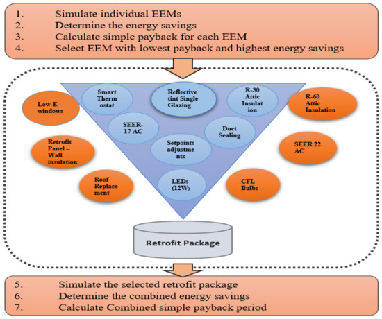
Figure 15.
Demonstration of automated process used to develop customized retrofit package of energy efficiency of individual EEMs for SFR buildings.
At the same time, other EEMs considered to have more extended payback periods, and the lowest energy savings with a higher cost are located outside of the tube. Though, some EEMs with a more extended payback period are still considered due to their higher potential energy savings and long-term cost savings. The combined EEMs are finally grouped as a retrofit package and further subjected to simulation analysis to determine energy savings and the total payback period. Also, the motive for running the package simulation was to estimate the overall economic potential of the SFR energy efficiency, while accounting for the overall effect of the selected EEMs on the building energy performance. Figure 15 outlined 7-steps for the determination of a recommended retrofit package. Next section provides a detailed analysis of energy-savings, the final recommended package, the payback period, and the cost associated with the retrofit package.
6.1. Cost Effectiveness of the Retrofit Improvement Package
This section uses a simple payback method to investigate the cost-effectiveness of the individual proposed EEM making up the retrofit package. The baseline building had an annual energy use of 19,081 kWh at a utility rate of $0.1142 kWh (Florida Power & Light Average) and an estimated yearly cost of $2104.7. The cost estimate for the improvement package stood at $16,891.5, with annual energy savings of 12,141.9 kWh (63.6%), referencing Table 9 below, excluding incentives, tax breaks, and loan solutions. The results also exclude the additional energy-saving measure using a solar PV system, discussed in this section as a support option to offset the remaining energy consumption of the main retrofit package.
The economic analysis calculations used first cost when a measure is chosen for efficiency improvement. The incremental first cost is used for a higher efficiency choice at a time of replacement. The reason for this alternative could be functionality or meeting market standards. For example, when an HVAC system is replaced for functionality or market standards, higher than minimum performance system could be selected. This choice might carry a cost premium. The economic analysis calculation in Table 10 shows a $3029.1 cost for choosing single-pane, reflective tint windows instead of double-pane tint windows for higher savings, as shown in Figure 13 due to the cost-effectiveness of single-pane tint. In Table 9, all individual improvements produced positive annual cash flows, including two significant capital intensive-measure (Window & Central pump, 17 SEER/9.6 HSPF). The Table further shows the annual energy and cost savings. Building envelope conditions and equipment for the existing building vary widely regarding the costs for some of the components. Instead of a specific set of improvements, the proposed combine retrofit improvement package, which yielded 63.6% of energy savings, is recommended and should be considered as a general guide for SFR building retrofit project.
Table 10.
Energy Use Intensity (EUI) for the implement Energy Efficiency. Measures (EEMs)/Retrofit Improvement Package
As presented at the bottom half of Table 9, additional energy-saving measure using solar PV panels is available to the owners who want to transform their building into zero or near-zero energy. Different options, according to system size, annual production, the number of panels for the owners to choose from depending on their needs. The assumptions for the payback calculation include panel type (single crystalline-13.8% efficient), installed panel cost – ($8.0/watt and $9.5/m²), and applied electrics cost $0.12/kWh. The potential cost savings and system payback calculations based on the annual energy production, the used electric cost, and the future cost escalation. Energy incentives, tax breaks, and loan solutions excluded from this analysis.
This measure should be considered after the main recommended retrofit improvement package shown in the first half of Table 9. Adding solar PV panels may incur an additional cost, and it will be beneficial to owners whose sole interest is high-performance building without much recourse to cost. Nonetheless, the benefits of solar addition may include, selling back to the grid some of the power generated as well as using the solar for electric vehicle (EV) charging. The extra generated energy could save some additional environmental costs and damages. Appendix A shows the detailed analysis of using solar PV energy generation as another alternative.
6.2. Energy Use Intensity (EUI) and Energy Savings
This section involves a review of historical total building energy use and cost, using the utility bill from the previous two years. The section defines the building’s Energy Use Intensity (EUI). The buildings EUI can be benchmarked against other similar buildings or the industry average. In the absence of a standard or benchmark, it isn’t straightforward to compare the energy uses between buildings [32]. Directly measuring the amount of energy used per a chosen period does not consider building size, configuration, or type of use. The use of Energy Use Intensity (EUI), i.e., referencing weather data, provides the means to equalize the way energy use is compared among various types of buildings and evaluating the manner of reducing overall energy consumption.
When using EUI, energy use is expressed as a function of a building’s total area or “footprint.” In the United States, typically, EUI expressed as the energy used per square foot (or its equivalent in meter square) of building square-footage per year. It is calculated by dividing the total gross energy consumed in one year (measured in kBtu or GJ) by the total gross square footage of the building. The current EUI of the simulated model from Revit stands at 13.1 kBtu/ft² (13.8 MJ/m²) compared to the baseline model EUI of 36.1 kBtu/ft²/year or 38.1 MJ/m²/year before the simulation analysis of the retrofit package.
Table 10 shows individual EEMs, which includes estimated energy use reduction (Projected Energy Savings per year). The saving is then multiplied to the total area (m²) of the entire SFR building surveyed across the entire sixty-seven counties in Florida. Furthermore, assuming various percentages of the savings can be realized by applying EEMs to the similar buildings in all of the counties, the savings is multiplied in 25%, 50%, and 75% and the corresponding values are listed in Table 10. accordingly.
7. Discussion
The main objective of this research includes identifying ways to improve the energy efficiency of single-family residential buildings through investigations of building envelope technologies, HVAC systems, and renewable energy technology measures. The study further proposes to develop EEMs capable of reducing energy consumption and minimize retrofit cost for the State of Florida as well as other hot-humid climate.
In an attempt to fulfill the stated objective, the authors conducted a comprehensive literature search to unravel what the other researchers have in the field done. The search was divided into three segments: retrofit techniques involving materials & methods, energy modeling, including techniques & tools, and economic analysis approaches. The idea of the survey was to determine the differing energy retrofit applications backed by authentic decision support tools. The findings portrayed a diverse nature of retrofit projects as well as influences of numerous uncertainty factors. Also, an advanced search on the actual energy-efficiency retrofit project in Florida suggests that it is crucial to secure all the key stakeholders’ support to formulate essential planning and decisions before the commencement of a project.
A series of activities, including a designed methodology took place to guide the implementation of this study. The research method adopted a broad approach targeted at improving the energy performance of the studied area. The study developed a Six-Step modeled framework consisting of the definition of the baseline model, verification of the model with actual building, identification of the EEMs, estimation of the EEMs, evaluation of how effective the EEMs are and the development of the retrofit package.
The identification of real data involving Florida’s SFR buildings constructed between 1950 and 1970 was the one most significant portion of the study. This search played a vital role, as the findings considered an integral part of the entire research.
Windows contributed as the largest source of cooling load, i.e., 30% of the home’s design cooling load was as a result of solar heat gain. Although some of the fenestration was double glazed, energy modeling indicated it is worth the effort and cost to replace the windows with single-pane reflective tint. Different types of windows, including; single-pane & double-pane clear, single-pane & double low-E, reflective single, and double tint glazing was subjected to multiple simulation analyses to unravel their energy-saving potentials. The single-pane reflective tint windows produced better energy savings of 2353 kWh (Figure 13), representing 20.2% with 11.6 years payback period. Upgrading the older and less efficient heat pump HVAC system with a newer 17 SEER/9.6 HSPF heat pump yielded immediate energy reduction benefit. The energy savings were 3879.3 kWh/year, about 33.2% (Figure 14) compared to the 14 SEER value. The payback was 13 years. The existing building had traditional T8 fluorescent lighting. The entire lighting system of the building was replaced with LED lighting. Changing the lighting system alone, yielded a savings of 2348 kWh/year, approximately 19.2% of the total energy consumption of the building. The introduction of occupancy sensors/dimmers boasted the energy savings further with an additional 298 kWh/year, representing 2.6% savings. The “Nest Smart Programmable Thermostat” also produced 7.8% savings per year. An extra no-cost measure, i.e., reducing heating setpoint and increasing cooling set points provided 2.6% savings as well.
Using solar PV to generate enough energy to offset the remaining energy end-use after the primary retrofit improvement measure was made available by the study. Different system sizes, application of solar PV systems and some improvement strategies have been investigated in the literature [99,100], annual production levels, and the number of PV panels are up for selection based on the owners’ discretion. Appendix A provides a detailed demonstration of solar PV alternatives.
Section 6.1 deals with the cost-effectiveness of the proposed retrofit improvement package, detailed in Table 9. The Table contained a retrofit package selected through the automated process discussed earlier in Section 6. The recommended package provided 63.6% of energy savings. By these results, the State of Florida would approximately save annual energy of 12,142 kWh for each single-family residential building built between 1950 to 1970. Also, the Energy Use Intensity (EUI) analysis conducted in Section 6.2. (detailed in Table 10) serves as a useful guide in applying the energy-savings to the overall State of Florida SFR buildings. It indicates how much energy the State can save going by this retrofit measure. For example, windows upgrade and lighting retrofit alone will save the state/counties as much as 5,766,776 MWh/year and 2,857,175 MWh/year, respectively.
The average monthly net energy consumption for the case study before the simulation exercise was 19,081 kWh/year compared to the simulated energy use of 12,142 kWh/year after the model calibration. This result is a perfect indication that the process can effectively be applied in other hot-humid climate zones.
Overall, the work done by other researchers reveals a diverse nature of energy efficiency retrofits and highly influenced by numerous uncertainty factors. The study addressed some varied issues of the energy retrofits by advocating for close collaboration between all the stakeholders from the early planning/design stage before the commencement of the project. This collaboration will help streamline the assumptions/requirements for the design, construction, and operational phases of each proposed energy retrofit projects. Also, some of the uncertainty factors have been resolved with the standardized process of selecting both EEMs/Retrofit package.
The future direction of the research would include comparing the energy efficiency practices, savings/cost reduction with different climates zones to determine market trend/value energy-efficiency retrofit projects from both the owner and tenant perspective. The future study will also focus on exploring different incentive packages to address the extended payback period for the benefits of applying the retrofit packages to low-income community dwellers.
8. Conclusions
This paper has identified potential energy efficiency improvement opportunities associated with older SFR buildings in hot-humid regions, particularly in the state of Florida. The methodology and results for the study document the technical and economic potentials of the electric end-use energy efficiency across the hot-humid climates for SFR housing stock. The paper presented energy savings and cost-effectiveness analysis of SFR buildings constructed between 1950 and 1970. The buildings are evaluated based on a survey via clustering data mining on Florida single-family residential buildings. The study of the EEMs effectiveness is performed utilizing Autodesk Revit, and a simplified six-step methodology. More than a thousand simulations analysis were conducted using various icons of Revit (energy analyze, heating & cooling, lighting, solar, etc.) to evaluate more than 40 EEMs to determine a recommended retrofit package.
The simple payback calculation revealed a fraction of the EEMs which met less than five -year threshold. This finding is due to the client’s demand for a shorter payback period, which may presumably be a barrier to the adoption of most of the EEMs. Four EEMs stood out as an excellent economic potential after applying the 5 years payback threshold, maintaining at least 90% of their energy-saving potential:
- Reducing heating set points & increasing cooling set points
- Installing programmable thermostats (when occupants not at home daytime)
- Lighting control- installing dimmers/occupancy sensors
- Adding radiant barriers
It was ideal for a further look into other individual EEMs upgrades, which had a more extended payback period but with excellent energy-saving potential and long-term cost benefits. Federal, states, or utility incentives are traditional ways to address the long payback periods market barrier and involves designing incentives that bring payback down to an acceptable range for owners. Emerging models for energy efficiency implementation may be able to address the long payback period and other market barriers. These emerging models include residential energy service companies, property-assessed clean energy financing, and on-bill financing. Though incentives and funding are out of focus for this paper, stakeholders, including SFR homeowners, can explore these incentive packages to address the extended payback problems.
The study presents a unique opportunity for the owners/stakeholders to choose from diverse retrofit options, including; the individual combination of EEMs, the entire retrofit package, or selecting a solar PV option as an addition to support either of the choice. The recommended package provided 63.60% of energy savings. By these results, the state of Florida, by extension, would save annual energy of 1128.0 kWh/m² for each single-family residential building built between 1950 to 1970 annually. By multiplying this result to the total square footage of the number of buildings surveyed across the state, the savings will amount to 3,476,535,167.1 kWh/m².
This study successfully developed a multifaceted framework that consolidates energy efficiency and cost-effectiveness into SFRs in hot-humid climates. The study also allows owners and the industry practitioners the needed techniques to undertake energy and cost-efficient retrofit project.
Author Contributions
The contributions of the author for this article includes: conceptualization, A.B.O.K. and N.V.T.; investigation, A.B.O.K.; validations, N.V.T. and N.H.; writing-original draft, A.B.O.K.; writing-reviews and editing, N.V.T., N.H. and A.B.O.K.; supervision, N.V.T. All authors have read and agreed to the published version of the manuscript.
Funding
This research was funded in part by the Open Access Subvention Fund and the John H. Evans Library, Florida Institute of Technology.
Conflicts of Interest
The authors declare no conflict of interest.
Appendix A. Solar PV Analysis
Additional energy reduction option, using solar PV is available to owners depending on the needs as stated in Section 6.1., bottom half of Table 10. To perform the analysis, we used the Revit Solar energy “analyze” tab. The roofing surfaces of the baseline model were analyzed to determine the surfaces exposed directly to the sunlight and those obstructed by shades. The sun settings include: "Multi-Day Solar Study, Date: 1/1/2019 – 12/31/2019, Time: 6:27 AM – 8: 13 AM, with one-hour interval. The tilt angle was set to 18° based on the site true north and pitch of the existing roof. Table A1 indicates the specific areas of the roof surfaces with direct exposure to sunlight. The main components of Table A1 include surface variables, shading variable, and the summary. Tilt (degrees) defines the angles of the solar panel installation; the solar exposure ranges from 100%, signifies fully exposed to direct sunlight at all year round and 0%, means in shadow. Obstruction shading ranges from 0.0%, indicating complete exposed to the environment while 100% means utterly obscured. Annual energy (kWh/m²) constitute the amount of DC power the solar panel produces while direction implies the orientation of the surfaces.
Table A1.
Photovoltaic surface analysis and power generation results.
Table A1.
Photovoltaic surface analysis and power generation results.
| Surface Variables | Shading Variables | Summary | ||||
|---|---|---|---|---|---|---|
| Type | Direction | Tilt (degrees) | Panel Area (m²) | Solar Exposure | Payback/ Surface(yrs.) | Annual Energy (kWh/m²) |
| Roof | S | 18 | 7.90 | 76.0% | 8.32 | 2046 |
| Roof | S | 18 | 2.32 | 75.9% | 8.32 | 607 |
| Roof | S | 18 | 3.62 | 75.9 % | 8.35 | 944 |
| Roof | S | 18 | 12.26 | 76.0% | 8.35 | 2012 |
| Roof | S | 18 | 3.32 | 75.5% | 8.31 | 922 |
| Roof | S | 18 | 6.04 | 75.8% | 8.34 | 1560 |
| Roof | S | 18 | 7.43 | 75.7% | 8.32 | 1913 |
| 32.51 | 8 yrs. | 10,004 | ||||
The second phase of the analysis focused on producing enough energy to offset the annual energy consumption of the baseline building after the improved retrofit package. The authors used Single-Crystalline PV panels for the study over Poly-Crystalline and Thin -Fin PV panel because of its ease of installation, maintenance and less labor/material cost. Figure A1 depicts the number of factors that include the size of the solar system to generate adequate power to meet the demands of the households, kilowatts hours of power needed for the house and the system size/number of solar panels to power the building under review. The system size reviewed ranges from 3.5 kW to 15 kW with average annual production ranges from 4954 kWh/m² to 21,234 kWh/², respectively as showed in Figure A1.

Figure A1.
Evaluated Photovoltaics (PV) alternatives.
References
- EIA, How Much Energy Is Consumed in U.S. Residential and Commercial Buildings? Available online: https://www.eia.gov/tools/faqs/faq.php?id=86&t=1 (accessed on 4 April 2018).
- EIA, Residential Energy Consumption Survey (RECS). Available online: https://www.eia.gov/emeu/consumption/index.html (accessed on 10 July 2018).
- USCB, American Housing Survey for United States: 2011–2013. Available online: https://www.census.gov/programs-surveys/ahs.html (accessed on 10 July 2018).
- Foley, H.C. Challenges and Opportunities in Engineered Retrofits of Buildings for Improved Energy Efficiency and Habitability. Available online: https://doi.org/10.1002/aic.13748 (accessed on 10 July 2018).
- Emrath, P.E.; Miller, J. How Much Energy Homes Use, and Why? Available online: http://www.nahbclassic.org/generic.aspx?sectionID=734&genericContentID=237901 (accessed on 10 July 2018).
- Wang, B.; Xia, X.; Zhang, J. A multi-objective optimization model for lifecycle cost analysis and retrofitting planning of building energy. Energy Build. 2014, 77, 227–235. [Google Scholar] [CrossRef]
- Betharte, O.; Najafi, H.; Nguyen, T. Towards net-zero energy buildings: A case study in humid subtropical climate. In Proceedings of the ASME 2018 International Mechanical Engineering Congress and Exposition, Pittsburgh, PA, USA, 9–15 November 2018; Volume 6A. [Google Scholar]
- D’Agostino, D.; Parker, D. A framework for the cost-optimal design of nearly zero energy Buildings (NZEBs) in representative climates across Europe. Energy 2018, 149, 814–829. [Google Scholar] [CrossRef]
- Fairey, B.; Parker, D. Cost-Effectiveness of Home Energy Retrofits in Pre-Code Vintage Homes in the United States; National Renewable Energy Lab. (NREL): Golden, CO, USA, 2012. [Google Scholar]
- Jafari, A.; Valentin, V.; Bogus, S.M. Assessment of social indicators in energy housing retrofits in construction. In Proceedings of the Construction Research Congress 2016, San Juan, Puerto Rico, 31 May–2 June 2016. [Google Scholar]
- McIlvaine, J.; Sutherland, K.; Martin, E. Energy Retrofit Field Study and Best Practices in a Hot-Humid Climate. Available online: https://www1.eere.energy.gov/buildings/publications/pdfs/building_america/energy_retrofit_study_hothumid.pdf (accessed on 11 July 2018).
- Silvero, F.; Montelpare, S.; Rodrigues, F.; Spacone, E.; Varum, H. Energy retrofit solutions for heritage buildings located in hot-humid climates. In Proceedings of the XIV International Conference on Building Pathology and Constructions Repair—CINPAR 2018, Florence, Italy, 20–22 June 2018. [Google Scholar]
- Burgett, J.M.; Chini, A.R.; Oppenheim, P. Specifying residential retrofit packages for 30% reductions in energy consumption in hot–humid climate zones. Energy Effic. 2013, 6, 523–543. [Google Scholar] [CrossRef]
- Ma, Z.; Cooper, P.; Daly, D.; Ledo, L. Existing building retrofits: Methodology and start-of-the-art. Energy Build. 2012, 55, 889–902. [Google Scholar] [CrossRef]
- Al-Saadia, S.N.J.; Al-Hajria, J.; Sayarib, M.A. Energy-efficient retrofitting strategies for residential buildings in hot climate of Oman. In Proceedings of the 9th International Conference on Applied Energy, ICAE2017, Cardiff, UK, 21–24 August 2017. [Google Scholar]
- Alam, M.; Zou Patrick, X.W.; Sanjayan, J.; Stewart, R.; Sahin, O.; Bertone, E.; Wilson, J. Guidelines for building energy efficiency retrofitting. In Proceedings of the Sustainability in Public Works Conference, Melbourne, Australia, 24–26 August 2016. [Google Scholar]
- Goldman, C.A.; Greely, K.M.; Harris, J.P. Retrofit experience in US multifamily buildings: Energy savings, costs and economics. Energy 1988, 13, 797–811. [Google Scholar] [CrossRef]
- Less, B.; Walker, I. Deep Energy Retrofit Performance Metric Comparison: Eight California Case Studies; Proceedings of the ACEEE Summer Study of Energy Efficiency in Buildings; Lawrence Berkeley National Lab: Berkeley, CA, USA, 2012. [Google Scholar]
- NREL, the National Residential Efficiency Measures Database. Available online: https://remdb.nrel.gov/ (accessed on 31 October 2018).
- Christensen, C.; Anderson, R. BEopt: Software for identifying optimal building designs on the path to zero net energy. In Proceedings of the ISES 2005 Solar World Congress, Orlando, FL, USA, 6–12 August 2005. Report Number: NREL/CP-550-37733. [Google Scholar]
- Rhodes, J.D.; Gorman, W.H.; Upshaw, C.R.; Webber, M.E. Using BEopt (EnergyPlus) with energy audits and surveys to predict actual residential energy usage. Energy Build. 2015, 86, 808–816. [Google Scholar] [CrossRef]
- Lee, S.H.; Hong, T.; Piette, M.A. Review of Existing Energy Retrofit Tools; Lawrence Berkeley National Laboratory (LBNL): Berkeley, CA, USA, 2014; Volume 33. [Google Scholar]
- Shabunko, V.; Lim, C.M.; Mathew, S. EnergyPlus models for the benchmarking of residential buildings in Brunei Darussalam. Energy Build. 2018, 169, 507–516. [Google Scholar] [CrossRef]
- Jafari, A.; Valentin, V.; Russell, M. Probabilistic life cycle cost model for sustainable housing retrofit decision-making. In Computing in Civil and Building Engineering; American Society of Civil Engineers: Reston, VA, USA, 2014; pp. 1925–1933. [Google Scholar] [CrossRef]
- WBDG Cost-Effective Committee. Use Economic Analysis to Evaluate Design Alternatives. Available online: https://www.wbdg.org/design-objectives/cost-effective/use-economic-analysis (accessed on 20 October 2018).
- Krarti, M. Energy Audit of Building Systems: An Engineering Approach, 2nd ed.; CRC Press, Taylor & Francis Group: Boca Raton, FL, USA, 2011. [Google Scholar]
- Verbeeck, G.; Hens, H. Energy savings in retrofitted dwellings: Economically viable? Energy Build. 2005, 37, 747–754. [Google Scholar] [CrossRef]
- Peterson, S.; Svendsen, S. Method for component-based economical optimization for use in design of new low–energy buildings. Renew. Energy 2012, 38, 173–180. [Google Scholar] [CrossRef]
- Kok, N.; Miller, N.G.; Morris, P. The Economics of Green Retrofits. J. Sustain. Real Estate 2012, 4, 4–22. Available online: http://onlinelibrary.wiley.com/doi/10.1002/cbdv.200490137/abstract (accessed on 20 October 2018).
- Nguyen, T.V.; Amoah, E.A. An approach to enhance interoperability of building information modeling (BIM) and data exchange in integrated building design and analysis. In Proceedings of the 36th International Symposium on Automation and Robotics in Construction (ISARC 2019), Banff, AB, Canada, 21–24 May 2019. [Google Scholar] [CrossRef]
- 2018 RSMeans Construction Project Costs. Available online: https://www.rsmeans.com/2018-construction-project-costs.aspx (accessed on 20 October 2018).
- Alachua County. Advanced Property Search. Available online: https://www.acpafl.org/searches/advanced-property-search/ (accessed on 1 November 2018).
- Baker County. Property Search. Available online: http://www.bakerpa.com/search.html (accessed on 1 November 2018).
- Bradford County. Interactive Record Search & GIS Mapping System. Available online: http://www.bradfordappraiser.com/GISv1/ (accessed on 1 November 2018).
- Brevard County. Real Property Search. Available online: https://www.bcpao.us/PropertySearch/#/nav/Search (accessed on 1 November 2018).
- Broward County. Property Search. Available online: http://www.bcpa.net/RecMenu.asp (accessed on 1 November 2018).
- Calhoun County. Property Data Search. Available online: https://qpublic.schneidercorp.com/Application.aspx?AppID=829&LayerID=15004&PageTypeID=2&PageID=6748 (accessed on 1 November 2018).
- Charlotte County. Real Property. Available online: https://www.ccappraiser.com/RPSearchEnter.asp? (accessed on 1 November 2018).
- Citrus County. Advanced Property Search. Available online: https://www.citruspa.org/_web/search/advancedsearch.aspx?mode=advanced (accessed on 1 November 2018).
- Hillsborough County. Advanced Property Search. Available online: https://gis.hcpafl.org/propertysearch/#/nav/Advanced%20Search (accessed on 1 November 2018).
- Pinellas County. Search Database. Advanced/Sales Criteria. Available online: https://www.pcpao.org/ (accessed on 6 November 2018).
- Polk County. Property Search. “Simple Query Search”. Available online: https://www.polkpa.org/CamaDisplay.aspx?OutputMode=Input&searchType=RealEstate&page=SimpleQuerySearch (accessed on 6 November 2018).
- Volusia County. Real Property Search. Available online: http://publicaccess.vcgov.org/Volusia/search/commonsearch.aspx?mode=realprop (accessed on 6 November 2018).
- Palm Beach County. Real Property Search Options. Available online: https://www.pbcgov.org/papa/Asps/GeneralAdvSrch/SearchPage.aspx?f=a (accessed on 6 November 2018).
- Pasco County. Record Search. Available online: https://search.pascopa.com/ (accessed on 6 November 2018).
- Escambia County. Tangible Record Search. Available online: https://www.escpa.org/CAMA/TangibleSearch.aspx (accessed on 6 November 2018).
- Wakulla County. Record Search. Available online: https://qpublic.schneidercorp.com/Application.aspx?AppID=836&LayerID=15205&PageTypeID=2&PageID=6831 (accessed on 6 November 2018).
- Manatee County. Property Search. Available online: https://www.manateepao.com/search/ (accessed on 6 November 2018).
- Sumter County. Real Property Record Search. Available online: http://www.sumterpa.com/GIS/ (accessed on 6 November 2018).
- St. Johns County, FL. Real Property Search. Available online: https://qpublic.schneidercorp.com/Application.aspx?App=StJohnsCountyFL&Layer=Parcels&PageType=Search (accessed on 18 November 2018).
- Hendry County. Interactive Record Search & GIS Mapping System. Available online: http://www.hendryprop.com/GIS/Search_F.asp (accessed on 18 November 2018).
- Glades County. Property record Search. Available online: https://qpublic.schneidercorp.com/Application.Aspx?AppID=818&LayerID=14562&PageTypeID=2&PageID=642 (accessed on 18 November 2018).
- Saint Lucie County. Property Search. Available online: https://www.paslc.org/property-search/real-estate/basic-site-address (accessed on 18 November 2018).
- Miami Dede County. Property Search. Available online: https://www.miamidade.gov/Apps/PA/propertysearch/#/ (accessed on 18 November 2018).
- Gadsden County. Property Search. Available online: https://qpublic.schneidercorp.com/Application.aspx?App=GadsdenCountyFL&PageType=Search (accessed on 25 November 2018).
- Oskaloosa County. Property Search. Available online: https://qpublic.schneidercorp.com/Application.aspx?App=OkaloosaCountyFL&PageType=Search (accessed on 25 November 2018).
- Hardee County. Search Record. Available online: https://qpublic.schneidercorp.com/Application.aspx?App=HardeeCountyFL&PageType=Search (accessed on 25 November 2018).
- Nassau County. Property Search. Available online: https://maps.nassauflpa.com/NassauSearch/IS_SearchResults2015/ShowIS_NewSearchResults2015Table.aspx (accessed on 25 November 2018).
- Santa Rosa County. Web Access to Property Records. Available online: https://www.srcpa.org/Search (accessed on 25 November 2018).
- Osceola County. Advanced Search. Available online: https://ira.property-appraiser.org/PropertySearch/ (accessed on 25 November 2018).
- Suwanee County. Available online: http://www.suwanneepa.com/GIS/Search_F.asp (accessed on 25 November 2018).
- Flagler County. Search Records. Available online: https://qpublic.schneidercorp.com/Application.aspx?App=FlaglerCountyFL&Layer=Parcels&PageType=Search (accessed on 2 December 2018).
- DeSoto County. Interactive Record Search & GIS Mapping System. Available online: http://www.desotopa.com/GISv1/ (accessed on 2 December 2018).
- Bay County. Property Record Search. Available online: https://baypa.net/search.html (accessed on 2 December 2018).
- Monroe County. Property Search. Available online: https://qpublic.schneidercorp.com/Application.Aspx?AppID=605&LayerID=9946&PageTypeID=2&PageID=4381 (accessed on 2 December 2018).
- Orange County. Property Searches/Record Search. Available online: https://www.ocpafl.org/searches/ParcelSearch.aspx (accessed on 2 December 2018).
- Okeechobee County. Record Search. Available online: http://g4b.okeechobeepa.com/gis/ (accessed on 2 December 2018).
- Leon County. Advanced Search. Available online: https://www.leonpa.org/pt/search/advancedsearch.aspx?mode=advanced (accessed on 2 December 2018).
- Madison County. Property Search. Available online: Https://qpublic.schneidercorp.com/Application.aspx?App=MadisonCountyFL&Layer=Parcels&PageType=Search (accessed on 2 December 2018).
- Gulf County. Property Search. Available online: https://qpublic.schneidercorp.com/Application.aspx?AppID=819&LayerID=15077&PageTypeID=2&PageID=6812 (accessed on 2 December 2018).
- Liberty County. Search. Available online: https://qpublic.schneidercorp.com/Application.aspx?AppID=828&LayerID=15003&PageTypeID=2&PageID=6744 (accessed on 15 December 2018).
- Clay Count. Property Search. Available online: https://qpublic.schneidercorp.com/Application.aspx?AppID=830&LayerID=15008&PageTypeID=2&PageID=6754 (accessed on 15 December 2018).
- Lake County Property Records Search. Available online: http://www.lakecopropappr.com/property-search.aspx? (accessed on 15 December 2018).
- Seminole County. Property Search. Available online: https://www.scpafl.org/ (accessed on 15 December 2018).
- Putnam County. Property Search. Available online: https://putapps.putnam-fl.com/palookup/main.php (accessed on 15 December 2018).
- Walton County. Property Record Search. Available online: https://qpublic.schneidercorp.com/Application.aspx?App=WaltonCountyFL&PageType=Search (accessed on 15 December 2018).
- Collier County. Search Database. Available online: http://www.collierappraiser.com/ (accessed on 4 March 2020).
- Lee County. Database Search/Property Data Search. Available online: https://www.leepa.org/Search/PropertySearch.aspx (accessed on 6 January 2019).
- Sarasota County. Advanced Property Search. Available online: https://www.sc-pa.com/propertysearch/Search/Advanced (accessed on 6 January 2019).
- Dixie County. Search Records. Available online: https://qpublic.schneidercorp.com/Application.aspx?AppID=867&LayerID=16385&PageTypeID=2&PageID=7230 (accessed on 6 January 2019).
- Franklin County. Property Search. Available online: https://beacon.schneidercorp.com/Application.aspx?AppID=816&LayerID=14540&PageTypeID=2&PageID=6405 (accessed on 7 January 2019).
- Columbia County. Real Property Record Search. Available online: http://columbia.floridapa.com/gis/ (accessed on 7 January 2019).
- Gilchrist County. Property Records. Available online: https://qpublic.schneidercorp.com/Application.aspx?App=GilchristCountyFL&Layer=Parcels&PageType=Search (accessed on 4 March 2020).
- Hamilton County. Property Search. Available online: https://beacon.schneidercorp.com/Application.aspx?AppID=817&LayerID=14544&PageTypeID=2&PageID=6409 (accessed on 6 January 2019).
- Holmes County. Search Records. Available online: https://qpublic.schneidercorp.com/Application.aspx?App=HolmesCountyFL&Layer=Parcels&PageType=Search (accessed on 8 January 2019).
- Jackson County. Search records. Available online: https://qpublic.schneidercorp.com/Application.aspx?AppID=851&LayerID=15884&PageTypeID=2&PageID=7081 (accessed on 8 January 2019).
- Hernando County. Where is My Property/Property Search? Available online: https://www.hernandocountygis-fl.us/propertysearch/ (accessed on 8 January 2019).
- Jefferson County. Property Search. Available online: https://qpublic.schneidercorp.com/Application.aspx?App=JeffersonCountyFL&PageType=Search (accessed on 10 January 2019).
- Lafayette County. Real Property Record Search. Available online: http://www.lafayettepa.com/GIS/Search_F.asp (accessed on 10 January 2019).
- Levy County. Record Search. Available online: https://qpublic.schneidercorp.comApplication.aspx?App=LevyCountyFL&PageType=Search (accessed on 10 January 2019).
- Taylor County. Record Search. Available online: https://qpublic.schneidercorp.com/Applicationaspx?AppID=792&LayerID=11749&PageTypeID=2&PageID=5268 (accessed on 10 January 2019).
- Union County. Interactive Record Search & GIS Mapping System. Available online: http://union.floridapa.com/GISv1/Search_F.asp (accessed on 10 January 2019).
- Washington County. Property Record Search. Available online: https://qpublic.schneidercorp.com/Application.aspx?App=WashingtonCountyFL&PageType=Search (accessed on 10 January 2019).
- Indian River County. Property Search. Available online: http://www.ircpa.org/Search.aspx (accessed on 10 January 2019).
- Marion County. Property Record Search. Available online: https://www.pa.marion.fl.us/SearchAgree.aspx (accessed on 15 January 2019).
- Martin County. Real Property Search. Available online: https://www.pa.martin.fl.us/ (accessed on 15 January 2019).
- Highland County. Search Real Estate. Available online: https://www.hcpao.org/Search (accessed on 15 January 2019).
- Gilchrist County. Property Search. Available online: https://qpublic.schneidercorp.com/Application.aspx?App=GilchristCountyFL&Layer=Parcels&PageType=Search (accessed on 15 January 2019).
- Najafi, H. Evaluation of alternative cooling techniques for photovoltaic panels. Ph.D. Thesis, The University of Alabama Libraries Digital Collections, Tuscaloosa, AL, USA, 2012. [Google Scholar]
- Najafi, H.; Najafi, B. Sensitivity analysis of a hybrid photovoltaic thermal solar collector. In Proceedings of the 2011 IEEE Electrical Power and Energy Conference, Winnipeg, MB, Canada, 3–5 October 2011; pp. 62–67. [Google Scholar]
© 2020 by the authors. Licensee MDPI, Basel, Switzerland. This article is an open access article distributed under the terms and conditions of the Creative Commons Attribution (CC BY) license (http://creativecommons.org/licenses/by/4.0/).